“Easy” Parameterized Verification of Cross Clock Domain Protocols

To appear in the Participants’s Proceedings of DCC: the Seventh International Workshop on Designing Correct Circuits (Satellite Workshop of ETAPS), 2006.

“Easy” Parameterized Verification of Cross Clock Domain Protocols Geoffrey M. Brown1 and Lee Pike2? 1

Indiana University, Bloomington [email protected] 2 Galois Connections, Inc. [email protected]

Abstract. This paper demonstrates how an off-the-shelf model checker that utilizes a Satisfiability Modulo Theories decision procedure and kinduction can be used for verification applications that have traditionally required special purpose hybrid model checkers and/or theorem provers. We present fully parameterized proofs of two types of protocols designed to cross synchronous boundaries: a simple data synchronization circuit and a serial communication protocol used in UARTs (8N1). The proofs were developed using the SAL model checker and its ICS decision procedures.

1

Introduction

This paper uses the bounded model checker and ICS decision procedures of SAL to develop fully parameterized proofs of two types of protocols designed to cross synchronous boundaries: a simple data synchronization circuit and a serial communication protocol, 8N1, used in UARTs.3 Protocols such as these present challenging formal verification problems because their correctness requires reasoning about interacting time events. The proofs discussed in this paper are parameterized by expressing temporal constraints as a system of linear equations. The proofs are “easy” in that they require few proof steps. For example, we have previously presented a proof of the biphase mark protocol [17], which is structurally similar to, though simpler than, 8N1. Our biphase mark proof required 5 invariants, whereas a published proof using PVS required 37; our proof required 5 proof directives (the proof of each invariant is automated), whereas the PVS proof initially required more than 4000 proof directives [1]. Our proofs are quick to check – a few minutes computing time, while one published proof of biphase mark required five hours. Furthermore, our proofs identified a potential bug: in verifying the 8N1 decoder, we found a significant error in a published application note that incorrectly defines the relationship between various real time parameters which, if followed, would lead to unreliable operation [2]. ?

3

The majority of this work was completed while this author was a member of the Formal Methods Group at the NASA Langley Research Center in Hampton, Virginia. The SAL specifications and proofs are available at http://www.cs.indiana.edu/ ∼lepike/pub pages/dcc.html.

1

din

dout

Receiver

Transmitter

rin

r1

rout

rclk

ain

aout

a1

tclk

Fig. 1. Synchronizer Circuit

The synchronizer circuit considered in this paper, illustrated in Figure 1, is constructed entirely of D-type flip-flops. The circuit, which is commonly used, allows a transmitter in one clock domain to reliably transmit data to a receiver in another clock domain irrespective of the relative frequencies of the clocks controlling the digital circuitry. This circuit allows the transmitter to send a bit (or in general a word) of data to the receiver through an exchange of “request” (rout, rin) and “acknowledgment” signals (aout, ain). A temporal illustration of the exchange between transmitter and receiver is presented in Figure 2. Each event initiated by the transmitter must propagate to the receiver and a response must be returned before the transmitter can initiate a new transfer. The protocol followed by the transmitter and receiver is a simple token passing protocol where the transmitter has the token and hence is allowed to modify its outputs only when ain = rout, and the receiver has the token and is allowed to read its input data din when rin != aout. For example, the transmitter sends data when rout = ain by setting dout to the value that it wishes to send and by changing the state of rout. Informally, the circuit satisfies a simple invariant: rin 6= aout ⇒ din = dout

(1)

Although the protocol is trivial, there is a fundamental issue that greatly complicates the behavior of the circuit – metastability. The fact that the two clocks rclk and tclk are not synchronized and may run at arbitrary relative rates means that we cannot treat the flip-flops in the circuit as simple delay elements. In particular, the correct behavior of a flip-flop depends upon assumptions about when its input may change relative to its clock. Changes occurring too soon before a clock event are said to violate the “setup time” requirement of the flip-flop while changes occurring too soon after a clock event are said to 2

rout,dout rin,din aout ain ~rout,dout ~rin,din ~aout

~ain rx time

tx time

Fig. 2. Synchronizer Circuit Timeline

violate the “hold time” requirement. Either violation may cause the flip-flop to enter a metastable state in which its output is neither “one” nor “zero” and which may persist indefinitely. In practice, probabilistic bounds may be calculated which define how long a metastable state is likely to persist. The illustrated circuit assumes that the time between two events on a single clock is long enough to ensure that the metastability resolution time (plus setup time) is shorter that the clock period with sufficiently high probability. While there have been other proofs of this circuit, they did not model the effects of metastability [3, 4]. An alternative approach has been proposed and is evidently used in a commercial tool to reproduce synchronization bugs by introducing random one-clock jitter in cross domain signals [5, 6]. A fundamental difference between our work and those cited is that we explicitly model timing effects and rely upon clearly stated timing assumptions to verify the circuit.

Frame 1

0

0

1

1

1

0

d0

1

d7

start bit

stop bit

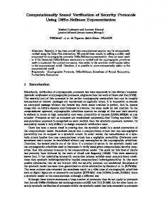
Fig. 3. 8N1 Data Transmission

Metastability also is an issue in the behavior of the 8N1 implementation in which a receiver must sample a changing signal in order to determine the boundaries between valid data. To motivate the design of the 8N1 protocol, 3

consider Figure 3 which illustrates the encoding scheme utilized by this protocol. In a synchronous circuit, the data and clock are typically transmitted as separate signals; however, this is not feasible in most communication systems (e.g., serial lines, Ethernet, SONET, Infrared) in which a single signal is transmitted. A general solution to this problem is to merge the clock and data information using a coding scheme. The clock is then recreated by synchronizing a local reference clock to the transitions in the received data. In 8N1 a transition is guaranteed to occur only at the beginning of each frame, a sequence of bits that includes a start bit, eight data bits, and a stop bit. Data bits are encoded by the identity function – a 1 is a 1 and a 0 is a 0. Consequently, the clock can only be recovered once in each frame in which the eight data bits are transmitted. Thus, the central design issue for a data decoder is reliably extracting a clock signal from the combined signal. Once the location of the clock events is known, extracting the data is relatively simple. Although the clock events have a known relationship to signal transitions, detecting these transitions precisely is usually impossible because of distortion in the signal around the transitions due to the transmission medium, clock jitter, and other effects. A fundamental assumption is that the transmitter and receiver of the data do not share a common time base and hence the estimation of clock events is affected by differences in the reference clocks used. Constant delay is largely irrelevant; however, transition time and variable delay (e.g., jitter) are not. Furthermore, differences in receiver and transmitter clock phase and frequency are significant. Any correctness proof of an 8N1 decoder must be valid over a range of parameters defining limits on jitter, transition time, frequency, and clock phase. Finally, any errors in detection can lead to metastable behavior as with the synchronization circuit. The temporal proofs presented in this paper may be reproducible using specialized real-time verification tools such as Hytech, TReX and Parameterized Uppaal (we leave it as an open challenge to these respective communities to reproduce these models and proofs in the those tools) [7–9]. However, a key difference is that SAL is a general purpose model checking tool and the real time verification we performed utilized the standard decision procedures. Furthermore, the proofs are not restricted to finite data representations – in the case of the data synchronization circuit our proofs are valid for arbitrary integer data. The remainder of the paper is organized as follows. In Section 2, we overview the language and proof technology of SAL. The modeling and verification of the synchronizer circuit is presented in Section 3. The model of the 8N1 protocol is presented in Section 4, and its verification is described in Section 5. In Section 6, we first describe how to derive error bounds on an operational model from a fullyparameterized one, and then we describe how this the operational model reveals errors in a published application note. We also mention future work. 4

2

Introduction to SAL

The protocols are specified and verified in the Symbolic Analysis Laboratory (SAL), developed by SRI, International [10]. SAL is a verification environment that includes symbolic and bounded model checkers, an interactive simulator, integrated decision procedures, and other tools. SAL has a high-level modeling language for specifying transition systems. A transition system is specified by a module. A module consists of a set of state variables and guarded transitions. Of the enabled transitions, one is nondeterministically executed at a time. Modules can be composed both synchronously (||) and asynchronously ([]), and composed modules communicate via shared variables. In a synchronous composition, a transition from each module is simultaneously applied; a synchronous composition is deadlocked if either module has no enabled transition. In an asynchronous composition, an enabled transition from one of the modules is nondeterministically chosen to be applied. The language is typed, and predicate sub-typing is possible. Types can be both interpreted and uninterpreted, and base types include the reals, naturals, and booleans; array types, inductive data-types, and tuple types can be defined. Both interpreted and uninterpreted constants and functions can be specified. This is significant to the power of these models: the parameterized values are uninterpreted constants from some parameterized type. Bounded model checkers are usually used to find counterexamples, but they can also be used to prove invariants by induction over the state space [11]. SAL supports k-induction, a generalization of the induction principle, that can prove some invariants that may not be strictly inductive. By incorporating a satisfiability modulo theories decision procedure, SAL can do k-induction proofs over infinite-state transition systems.4 Let (S, I, →) be a transition system where S is a set of states, I ⊆ S is a set of initial states, and → is a binary transition relation. If k is a natural number, then a k-trajectory is a sequence of states s0 → s1 → . . . → sk (a 0-trajectory is a single state). Let k be a natural number, and let P be property. The k-induction principle is then defined as follows: – Base Case: Show that for each k-trajectory s0 → s1 → . . . → sk such that s0 ∈ I, P (sj ) holds, for 0 ≤ j < k. – Induction Step: Show that for all k-trajectories s0 → s1 → . . . → sk , if P (sj ) holds for 0 ≤ j < k, then P (sk ) holds. The principle is equivalent to the usual transition-system induction principle when k = 1. In SAL, the user specifies the depth at which to attempt an induction proof, but the attempt itself is automated. The main mode of user-guidance in the proof process is in iteratively building up inductive invariants. While arbitrary LTL safety formulas can be verified in SAL using k-induction, only state predicates may be used as lemmas in a k-induction proof. Lemmas strengthen 4

We use SRI’s ICS decision procedure [12], the default SAT-solver and decision procedure in SAL, but others can be plugged in.

5

the invariant. We have more to say about the proof methodology for k-induction in Section 5.

3

Modeling and Verification of the Synchronizer Circuit

In this section we use a simple synchronizer circuit to illustrate the various modeling techniques used in this paper through the creation of successively more accurate models of the synchronizer circuit utilizing the transition language of SAL. In order to make the problem slightly more interesting, we generalize the data transfered by the circuit (din, dout) to arbitrary integers. Our initial model for the system of Figure 1 consists of two asynchronous processes – a transmitter (tx) and a receiver (rx). system : MODULE = rx [] tx;

Thus, the transmitter and receiver execute in an interleaved fashion and at arbitrary rates; however, each is made up from several processes that are composed synchronously (i.e., operate in lock step). For example, the transmitter is composed of an “environment”, which follows the basic protocol described above, and two instantiated flip-flops modules (described below) with their inputs and outputs suitably renamed. tx : MODULE =

(

(RENAME d TO aout, q TO a1 IN FF) || (RENAME d TO a1, q TO ain IN FF) || tenv);

Our initial flip-flop model in Figure 4 has no provision for capturing timing constraints. Indeed, its behavior is simply an assignment that copies input d to output q without any reference to an underlying clock. Our models depend upon synchronous composition to force the flip-flops comprising the transmitter (and receiver) to execute in lock step.

FF : MODULE = BEGIN INPUT d : BOOLEAN OUTPUT q : BOOLEAN INITIALIZATION q = FALSE TRANSITION q’ = d END;

Fig. 4. Flip Flop

As mentioned, the transmitter’s environment, shown in Figure 5, is constrained to obey the underlying protocol. There are two subtle points in this definition – we allow the data transmitted to take any randomly selected integer 6

value, and we allow the transmitter to “stutter” indefinitely when it is allowed to transmit a new value (stuttering is expressed by guard --> where guard is a boolean expression). The syntax var IN range defines a non-deterministic choice chosen from the set range. The infinite state model checker of SAL that enables our verification of timing constraints also enables verification with unbounded variables.

tenv : MODULE = BEGIN INPUT ain : BOOLEAN OUTPUT rout : BOOLEAN OUTPUT dout : INTEGER INITIALIZATION dout IN { x : INTEGER | TRUE }; rout = FALSE TRANSITION [ TRUE --> [] rout = ain --> rout’ = NOT rout; dout’ IN {x : INTEGER | TRUE }; ] END;

Fig. 5. Transmitter’s Environment

The receiver is similarly composed of an environment, flip-flops, and a data latch (the flipflop module in which the input and output variables are generalized to arbitrary integers). rx : MODULE = ((RENAME d TO rout, q TO r1 IN FF) || (RENAME d TO r1, q TO rin IN FF) || (RENAME d TO dout, q TO din IN LATCH) || renv);

The receiver environment module non-deterministically stutters or echos rin. renv : MODULE = BEGIN INPUT rin : BOOLEAN OUTPUT aout : BOOLEAN INITIALIZATION aout = FALSE TRANSITION aout’ IN {aout, rin} END;

The defined circuit can be verified by induction over the (infinite) state space using the bounded model checking capabilities of SAL. In its current form, this circuit requires only straight induction (k = 1) for verification. Because the circuit implements a token passing protocol, a token counting lemma like the one in Figure 6 is key to its verification. Here, a “token” exists where the input and output to a flip-flop differ or where the receiver or transmitter environments are enabled to receive or send a value respectively; the syntax is the LTL temporal 7

logic where the G operator denotes that its argument holds in all states in a trajectory through the transition system. This lemma is used to prove the key theorem using simple induction:

changing(i : BOOLEAN, o : BOOLEAN) : [0..1] = IF (i /= o) THEN 1 ELSE 0 ENDIF; l1 : LEMMA system |- G(changing(rin, r1) + changing(r1, rout) + changing(rout,ain) + changing(ain, a1) + changing(a1, aout) + changing(aout,NOT rin) (dout = din));

Not surprisingly, both l1 and Sync Thm can be verified quickly by SAL; however, the model as given does not capture any of the flip-flop timing requirements nor does it model any of the negative effects due to violating these requirements. In the following, we present a model that captures some of these requirements and allows us to verify the circuit even in the face of failures to meet these requirements. We begin by modeling clocks. The transmitter and receiver are each composed with a local clock that regulates when that component may execute. The system we are developing has the following form: (rx || rclock) [] (tx || tclock)

The basic idea, described as timeout automata by Dutertre and Sorea, is that the progress of time is enforced cooperatively (but nondeterministically) [13, 14]. The receiver and transmitter have timeouts, rclk and tclk, that mark the realtime at which they will respectively make transitions (timeouts are always in the future and may be updated nondeterministically). Each respective module representing the receiver and transmitter is allowed to execute only if its timeout equals the value of time(rclk, tclk), which is defined to be the minimum of all timeouts. time(t1 : TIME, t2: TIME): TIME = IF t1 [] dclk = dclk’ AND d /= d’ --> ts’ = time(dclk,qclk) + stime [] dclk = dclk’ AND d = d’ --> ] END;

Fig. 10. Constraint Module

r1 is assigned rout or the local timer must be active. Finally, if neither condition occurs, the constraint module allows tx2 to execute. To constrain the three possible sources of non-deterministic behavior, there are three constraint modules with the local timers r1ts, a1ts, and d1ts monitoring changes on rout, aout, and dout, respectively. The three constraint modules utilize two settling constants TSETTLE (for rout and dout) and RSETTLE (for aout). In verifying the circuit, we found that correct behavior depends on establishing a relationship between settling times and clock periods. In particular, the settling time of the transmitter must be less than the clock period of the receiver (and vice versa). Violating these assumptions has the effect of “injecting” additional tokens into the circuit whenever metastability occurs. Thus, we performed verification under the following assumptions.

TSETTLE RSETTLE

: { x : TIME | 0