Jul 16, 2008 - these two values would be equal (Pythagoras). Thus, if the squared ... tain reduction of the approximation error (in expectation or with a certain ...
Aiming for a Theoretically Tractable CSA Variant by Means of Empirical Investigations ∗
Jens Jägersküpper & Mike Preuss TU Dortmund Fakultät für Infomatik 44221 Dortmund, Germany
ABSTRACT Evolution Strategies (ES) for black-box optimization of a function f : Rn → R are investigated. Namely, we consider the cumulative step-size adaptation (CSA) for the variance of multivariate zero-mean normal distributions, which are commonly used to sample new candidate solutions within Evolution Strategies (ES). Four simplifications of CSA are proposed and investigated empirically and evaluated statistically. The background for these four new CSA-derivatives, however, is not performance tuning, but our aim to accomplish a probabilistic/theoretical runtime analysis of an ES using some kind of a CSA in the near future, and a better understanding of this step-size control mechanisms. Therefore, we consider two test problems, namely the Sphere function without and with Gaussian noise.
Categories and Subject Descriptors F.2 [Analysis of Algorithms and Problem Complexity]: Experimental Analysis; G.3 [Probability and Statistics]: Probabilistic Algorithms; G.1.6 [Optimization]: Sphere Function; I.2.8 [Problem Solving, Control Methods, and Search]: Evolution Strategies
General Terms Algorithms, Experimentation, Performance, Theory
Keywords Empirical Analysis, Evolution Strategies, Sphere Function
1.
INTRODUCTION
Within this work, we try to establish an alternative way towards theoretical tractability of evolution strategies (ES), ∗supported by the German Research Foundation (DFG) through the collaborative research center “Computational Intelligence” (SFB 531)
Permission to make digital or hard copies of all or part of this work for personal or classroom use is granted without fee provided that copies are not made or distributed for profit or commercial advantage and that copies bear this notice and the full citation on the first page. To copy otherwise, to republish, to post on servers or to redistribute to lists, requires prior specific permission and/or a fee. GECCO’08, July 12–16, 2008, Atlanta, Georgia, USA. Copyright 2008 ACM 978-1-60558-130-9/08/07…$5.00.
503
namely of those employing the cumulative step-size adaptation (CSA) for determining the expected length of the next search step. Although we aim at theoretical advances, our approach is purely empirical at first, to be carried on with a proper analysis later, once a simplified, but still functionally similar algorithm is found. Thus, instead of creating a complex new step-size adaptation, we follow an unorthodox approach by trying to dissect one, namely CSA, into parts, which may then be replaced by alternative mechanisms we regard as better suited for a probabilistic/theoretical analysis. While doing so, we heavily rely on experimentation to assess how far we depart from the original algorithm when substituting mechanisms by simpler ones. At the same time, we aim at better understanding the ‘core’ mechanisms of the original algorithm. Furthermore, a simplified algorithm may also be interesting for practitioners, as simple methods often spread much faster than their complicated counterparts, even if the latter have slight performance advantages. However, in our case the surrogate methods hardly differ concerning implementation requirements but rather in the accessibility towards theoretical analysis. In a sense, our approach can be seen as algorithm reengineering, a viewpoint which is to our knowledge uncommon in meta-heuristics, and especially in evolutionary computation (EC). Therefore, we strive for making a methodological contribution that hopefully inspires other researchers to follow a similar path. Within the domain of numerical black-box optimization, the covariance matrix adaptation evolution strategy (CMA-ES) of Hansen and Ostermeier [1996] is regarded as one of the most efficient modern methods, cf. the list of over 100 references to applications of CMA-ES compiled by Hansen [2008]. Although empirical evidence shows that this evolutionary algorithm (EA) performs very well on many benchmark and practical optimization problems, its theoretical foundations are rather weak, unfortunately a common situation in EC. The CMA-ES features two original mechanisms when compared to naive ES: the covariance matrix adaptation and the cumulative step-size adaptation (CSA). While the former develops, in some sense, a quadratic model like the well-known BFGS gradient-based optimization algorithm (cf. Nocedal and Wright [1999] for instance), which is especially useful on ill-conditioned optimization problems, it is the duty of the latter to cope with a difficulty that emerges in every real-valued black-box optimization algorithm, namely the adaptation of step-sizes when approaching an optimum.
Evolutionary algorithms usually strive for learning good step-sizes, which may be implemented by, e.g., self-adaptation or simple success-based rules, the most prominent of which may be the 15 -rule to increase/decrease step sizes if more/less than 51 of the performed test steps are successful. This simple deterministic adaptation mechanism (which is due to Rechenberg/Schwefel), has already been the subject of a probabilistic analysis of the (random) number of steps necessary to reduce the approximation error in the search space. The first results from the viewpoint of analyzing ES like “usual” randomized algorithms were obtainedP for the 2 simplest quadratic function, namely x 7→ x> Ix = n i=1 xi (which is usually called Sphere in EC), in [J¨ agersk¨ upper, 2003]. This analysis has been extended to quadratic forms with bounded condition number, on the one hand, and on the other hand to a certain class of ill-conditioned quadratic forms (parameterized in the dimensionality of the search space) for which the condition number grows as the dimensionality of the search space increases [J¨ agersk¨ upper, 2005]. The main result of the latter work is that the performance degrades in the same order as the condition grows. This drawback has already been noticed before in practical EC, of course. As noted above, within CMA-ES the cumulative step-size adaptation (CSA) is used, which is neither a self-adaptive mechanism nor based on a success rule. Here, we exclusively deal with this CSA mechanism and, consequently, again assume a (spherically) symmetric problem where the CMA mechanism is dispensable. Furthermore, as opposed to virtually all theoretical work which goes for the limit case (n → ∞), we explicitly focus on practically relevant dimensions. As it may be debatable what ‘relevant’ is, we give a 3-fold categorization to be used in the following. Problems with up to 7 dimensions are seen as small (S), whereas the medium sized ones (M) from from 8 to 63 dimensions are to our knowledge of the highest practical importance. Problems with 64 dimensions and beyond are termed large (L). As the efficiency of CSA has been disputed for noisy problems (Beyer and Arnold [2003b]), these also pose an interesting test case for the simplified CSA-derivatives and are thus additionally considered in this investigation. Indeed, it turns out that at least one of our CSA-derivatives displays a surprising behavior under noise. Within the following section, the original CSA for σ-adaptation is described in detail. The newly “re-engineered” four CSA-derivatives are presented in Section 3, and their technical details and differences are discussed in Section 4. We then experimentally compare the five CSA-variants in Section 5.1 and present our conclusions in Section 6.
2.
Since the steps’ directions are random, considering just the last two steps, namely their correlation, does not enable a smooth σ-adaptation because of large variations in the random angle between two steps. Thus, in each iteration, the correlation of the step just taken in this iteration and the so-called evolution path is considered. Essentially, the evolution path is a recent part of the trajectory of candidate solutions generated during the run of the ES. Considering the complete trajectory is not the most appropriate choice, though. Rather, a particular number of steps (amount of the recent history of the search) should be considered. Throughout this paper, we employ a (1,5) Evolution Strategy as basic algorithm. That is, in each iteration five candidate solutions are generated, each independently in the same way, namely by adding a random vector to the current candidate solution each component of which is chosen i.i.d. according to a zero-mean normal distribution with variance σ 2 . The best of those five samples becomes the next candidate solution—irrespective of whether this best of five amounts to an improvement or not. (CSA is not designed for elitist selection where the best sample becomes the next candidate solution only if it is at least as good.) The reason for this choice is that, according to Beyer [Beyer, 2001, p. 73], for this so-called comma-selection five samples are most “effective” (allow maximum progress per sample/f -evaluation)— given that σ could be adapted optimally. Thus, differences in the adaptations’ abilities (to choose σ as close to optimal as possible) should be most noticeable for this choice. In the following, we denote by “CSA” the original version as proposed by Hansen and Ostermeier. Therein σ is adapted continuously, namely after each iteration of the evolution loop. The deterministic update of the evolution path p ∈ Rn after the ith iteration works as follows: p (1) p[i+1] := (1 − cσ )p[i] + cσ (2 − cσ ) · m[i] /σ [i] where m[i] ∈ Rn denotes mutation vector actually selected in the ith step. Recall that m[i] is one of the five vectors each of which was independently chosen according to a zeromean multivariate normal distribution with standard deviation σ [i] . Note that the length of such a vector follows a scaled (by σ) χ-distribution. (We let χ ¯ denote the expectation of the χ-distribution.) Initially, p[0] is chosen as the all-zero vector. The σ-update is done deterministically as follows: � [i+1] �� � |p | cσ · −1 (2) σ [i+1] := σ [i] · exp dσ χ ¯
CUMULATIVE STEP-SIZE ADAPTATION
Originally, CSA was proposed by Hansen and Ostermeier [1996].The underlying idea is as follows: Consecutive steps of an iterative direct-search method should be orthogonal. Therefore, one may recall that steps of steepest descent (a gradient method) with perfect line search (i.e., the truly best point on the line in gradient direction is chosen) are orthogonal when a positive definite quadratic form is minimized. Within CSA the observation of positively [negatively] correlated successive steps is taken as an indicator that the step-size is too small [resp. too large]. As a consequence, the variance (actually the standard deviation σ) of the multivariate normal distribution is increased [resp. decreased].
504
In Eqn. (1), the fixed parameter cσ ∈ (0, 1) determines the weighting between the recent history of the optimization √ and its past in the evolution path p. It is chosen as 1/ n as √ and Ostermeier [1996]. Since √ suggested by Hansen (1 − 1/ n)i = 0.5 for i � n · ln 2 (as n grows), the√half-live of a step within the evolution path is roughly √ 0.5 n iterations for small dimensions and roughly 0.7 n for large n. (In fact, this √ is the reason why we will choose the “phase length” k as d n e a priori for the simplified versions which are to be described in the next section.) The fixed parameter “dσ ” in Eqn. (2) is called “damping factor”. We used dσ := 0.5 because this leads to a better performance than dσ ∈ {0.25, 1} for the considered function scenario. Some sort of interdependence between dσ and cσ appears likely, and moreover, an optimal choice may depend (among others) on the function to be optimized.
3.
FOUR CSA-DERIVATIVES 100
In this section we introduce four simplifications of the original CSA, created by subsequently departing further and further from the defining equations (1) and (2). The first simplification (common to all four variants) will be to partition the course of the optimization into phases of a fixed length. Such a partitioning of the process has turned out useful in former analysis (cf. Droste et al. [2002], J¨ agersk¨ upper [2007] for instance). Thus, all variants to be introduced will use phases (with a fixed length), after each of which σ is adapted—solely depending on what happened during the phase, respectively. The second simplification to be introduced is as follows: Rather than comparing the length of the displacement (vector) of a phase with the (expected) length that would be observed if the steps in the phase were orthogonal, the actual correlations of the selected mutation vectors of a phase in terms of orthogonality are considered directly and aggregated into a criterion, which we will call correlation balance.
90
2.5
sigma_up
60
80
45
2.0
70
60
38
35 1.5
50
33
30
40
27
80
100
30
2
pCSA. The “p” stands for phased. √The run of the ES is
4
6
8
10
log(dim, 2)
partitioned into phases lasting k := d ne steps, each. (This phase length will also be used for the following three algorithms.) In each phase, the vector corresponding to the total movement (in the search space) of the steps in this phase is considered. The √ length of this displacement vector is com¯ where χ ¯ is the expectation of the pared to ` := k · σ · χ, χ-distribution with n degrees of freedom. Note that ` equals the diameter of a k-dimensional cube with edges of length σ · χ, ¯ and that σ · χ ¯ equals the expected step length used in the phase. Thus, if all k steps had the expected length, and if they were completely orthogonal, then the length of the displacement vector in such a phase would just be equal to `. Thus, depending on whether the actual length is larger [or smaller] than `, σ is considered as too small (because of positive correlation) [resp. as too large (because of negative correlation)]. Then σ is scaled up [resp. down] by a fixed scaling factor larger than one [resp. its reciprocal]. The factor 1 + 1/n1/4 by which the σ-scaling was actually done was determined by a parameter scan (cf. Figure √ 1)—whereas the phase length k was chosen a priori as d ne (for the reason confer the discussion in the section on the original CSA). All in all, pCSA is pretty close to the original CSA.
Figure 1: Parameter scan of σ-scaling factors for pCSA over 2 to 1024 dimensions. Number of steps devided by dimensionality. The solid line represents the chosen factor 1 + 1/n1/4 .
[negative], the σ used in the respective phase is considered as too small [resp. as too large]. Hence, σ is scaled up [resp. down] after the phase by some predefined factor larger than one [resp. by the reciprocal of this factor]. A parameter scan has shown that this scaling factor should again be chosen as 1 + 1/n1/4 —just as for pCSA, cf. Fig. 1 and Fig. 2. (The name CBA2 has historical reasons; the first CBA-design considered only the k − 1 sequent pairs of vectors instead of all � k pairs.) 2
CBA3. CBA3 differs from CBA2 as � follows: Rather than k
considering just the signs of the 2 correlation values, the actual values are added up1 . Then, depending on whether their sum is positive [negative], σ is scaled up [resp. down] in the same way as in CBA2. The idea behind this modification is that this sum aggregates more information than the criterion in CBA2. (More information, however, need not necessarily be advantageous. In this case, however, it is as we will see.)
sCSA. “sCSA” stands for simplified CSA, actually simplified pCSA. Now, sCSA differs from pCSA in that the actual lengths of the k steps are considered (rather than the expected length σ · χ ¯ for each step in the phase). Namely, the squared length of the phase’s displacement vector is compared to the sum s of the squared lengths of the k steps. If the k steps in a phase were completely orthogonal, then these two values would be equal (Pythagoras). Thus, if the squared length of the total movement is larger than s, then σ is up-scaled; if it is smaller than s, then σ is down-scaled (as within pCSA, respectively).
4.
DISCUSSION OF THE CSA-VARIANTS
First of all note that up to 4-dimensional search space— √ actually, when the phase length k = d ne equals two—the criteria in CBA2, CBA3, and sCSA are equivalent. The partition of the course of the optimization into phases (here, of the same length) in each of which σ is kept unchanged and after each of which σ is deterministically updated solely depending on what happened in that phase, enables the following line of reasoning: First, one shows that the adaptation is such that after each phase the “right” decision is made (with high probabil-
CBA2. “CBA” stands for correlation-balance adaptation. After each phase, the k vectors that correspond to the k movements in the phase are considered. For each pair of these k �vectors the correlation is calculated, so that we obtain k = k(k −1)/2 correlation values (actually, the inner prod2 ucts suffice). If the majority of these values are positive
1
505
correlation of vectors x and y is
, |x|·|y|
equals cos (x∠y)
k 2
� /2 or smaller. There are strong bounds on the deviation of the actual sum of 0-1-variables from the expected sum, in particular when the variables are independent—which is not the case in CBA2, unfortunately; but this can be overcome by stochastic dominance arguments. All in all, CBA2 is a candidate for a theoretical analysis of the runtime of an ES using this simplified variant of CSA. Of course, it was an open question, whether CBA2 performs well compared to the original CSA and also compared to the other three simplifications thereof. Thus, we decided for an experimental comparison. Note that the number of f -evaluations (which is five times the number of iterations) is the only performance measure which will be considered in the following comparison of the five σ-adaptation mechanisms.
100
90
2.5
80
sigma_up
33 70
2.0
60
33 50
31 30
1.5
33
60 50 80
2
40
27
40
5.
25 30
4
6
8
5.1
10
EXPERIMENTAL INVESTIGATION OF THE CSA-VARIANTS Runtime and mutation strength
To find out the potentials of the previously described σadaptation mechanisms, we focus on the simplest unimodal function scenario, namely the minimization of the distance from a fixed point. This is equivalent to the minimization of a perfectly conditioned positive definite quadratic Pn form. 2 One of these functions, namely x 7→ x> Ix = i=1 xi , is very often considered in EC and has been named Sphere (level sets of such functions form hyper-spheres).
log(dim, 2)
Figure 2: Parameter scan of σ-scaling factors for CBA2 including the chosen factor 1 + 1/n1/4 .
ity), i.e., the changes of σ are such that the step lengths are better [at least as well] adapted to the current optimization situation than [as] in the previous phase. Second, one shows that this results in σ being (actually, becoming and remaining) close to optimal, and that each such phase causes a certain reduction of the approximation error (in expectation or with a certain probability), so that the (expected) number of phases required for a predefined reduction of the approximation error can be estimated. Third, one has to show that the probability of a “wrong” decision is small enough, such that a sequence of wrong decisions is almost never observed (at least a very rare event). Finally, one has to show that when something does go wrong in a phase, then this phase is only moderately harmful, i.e., if (at all) the approximation error is increased, then only by a small amount (again with very high probability). In contrast, for the original CSA, all steps are represented in the evolution path. So, in the case a very bad step happens (which might be a rare event), this bad step may influence the adaptation for a long period, depending on how bad it was (and on the parameters cσ and dσ , of course). To cover such effects in a probabilistic analysis is much more involving than the line of reasoning about phases described above. Note that, because of the random direction of the trial steps, the probability that two steps are exactly orthogonal is zero. Thus, two steps are a.s. either positively or negatively correlated so that in a phase of k steps the number of � positively correlated pairs of steps is a.s. equal to k2 minus the number of negatively correlated pairs.� Thus, for a theoretical analysis of CBA2, for each phase k2 0-1-variables can be defined. Each of these indicator variables tells us whether the respective pair of steps is positively correlated (“1”) or not (“0”). Recall that in CBA2 the σ-adaptation is based on whether the sum of these indicator variables is larger than
Experiment. Do the four proposed CSA-derivatives perform similar to the original CSA?
Pre-experimental planning. In addition to the adaptation rule and the phase length, the scaling factor by which σ is increased or decreased after a phase had to be fixed. After some testing we decided to apply the factor 1 + 1/n1/4 , which has been determined for pCSA and CBA2 by means of parameter scans (Figure 1), also for sCSA and CBA3.
Task. The hypothesis is that the five σ-adaptation mechanisms perform equally well in terms of number of iterations. As the data can not be expected to be normally distributed, we compare two variants, namely their runtimes, by the Wilcoxon rank-sum test (as implemented by “wilcox.test” in “R”), where a p-value of 0.05 or less indicates a significant difference, i.e, we reject the hypothesis of equal performance.
Setup. The initial distance from the optimum is 220 and the stopping criterion is a distance of less than 1 from the optimum/origin, i.e., we measure the number of iterations to halve the approximation error in the search space 20 times. The initial σ is set to 220 · 1.225/n in each case. We investigate ten search-space dimensions, namely n = 2i for i ∈ {1, 2, . . . , 10}. Each of the five σ-adaptation mechanisms is run 1001 times. (101 runs for each σ-scaling factor in the parameter scans; Fig. 1 and Fig. 2).
Results. Figure 3 displays median runtimes and hinges for four of the five CSA-variants. The lower and upper hinges refer to the lower quartile (25th percentile) and the upper quartile (75th percentile), respectively. Although CBA3 and sCSA (green in Figure 3) differ for a phase length k ≥ 3, they
506
CSA 2
CSA 16
2 1 0 −1 PCSA 2
SCSA 2
6 4 2 0 −2
CBA3 2
6 4 2 0 −2
CBA2 2
6 4 2 0 −2
PCSA 16
6 4 2 0 −2
ld(sigma*dimension/distance)
ld(sigma*dimension/distance)
6 4 2 0 −2
2 1 0 −1 SCSA 16
2 1 0 −1 CBA3 16
2 1 0 −1 CBA2 16
2 1 0 −1 0
50
100
150
0
steps
100
200
300
400
500
steps
Figure 4: Normalized σ (w.r.t. dimensionality and distance from optimum) in a typical run (i.e. median runtime) on 2-dimensional (S) Sphere Problem
Figure 5: Normalized σ in a typical run of each variant on 16-dimensional (M) Sphere
cannot be visually distinguished here. Unfortunately, it is an open question why. Additionally, we depict the σ-adaptation within typical runs (i.e. median runtime) in the Figures 4, 5, and 6. Note that σ is considered well-chosen (after normalization) if contained within the two horizontal lines; the lines correspond to a normalized σ of 1.0 (blue) and 2.0 (red).
Actually, for 2-dimensional search space, when we multiply the number of steps in each of the 1001 CSA-runs by 3, the Wilcoxon test can no longer tell us a significant difference between CSA and CBA2 (p-value increases to 0.85). In four dimensions, the test cannot tell a significant difference for a factor of 2.3 (p-value 0.78), and for eight dimensions the factor 1.618 does not lead to a significant difference (pvalue 0.095). Since the p-values drop below 5% again when the fators are increased, resepectively, we may conclude that CBA2 is slower than CSA by roughly a factor of three in two dimensions, by roughly a factor of 2.3 in four dimensions, and by roughly 62% in eight dimensions. As can be seen in Figure 7, then the factor between CSA and CBA2 drops almost linearly down to roughly 13% for 1024-dimensional search space (p-value 0.75 when multiplying each of the 1001 runtimes of CSA by 1.13). So, at least concerning the runtimes pCSA behaves much more like the original CSA than CBA2, cf. Figure 7 again. Concerning the obtained performance differences, we assume that CBA2—the only variant for which a theoretical analysis seems currently feasible—still works reasonably well to legitimate such an analysis, at least for the practically relevant (M) and large (L) dimensions. In the M+L domain, the number of f -evaluations to spend is increased by a maximum of 62%, getting less for larger dimensions down to 13% for 1024D. Clearly, the differences in the runtimes are due to differences in the ability to adapt σ. Therefore, we consider the normalized σ ∗ , i.e., σ times the dimensionality divided by the distance from the optimum point. Note that, for the simple function scenario considered, for each dimension there is a unique σ ∗ resulting in maximum expected reduction of the approximation error per step. Figures 4, 5, and 6 show the course of σ ∗ for each of the five CSA-variants for a typical run in dimension 2 (very small), 16 (of practical interest), and 1024 (very large), respectively. In the following table, the log-mean of σ ∗ , i. e. exp(mean(ln σ ∗ )), for these runs are given (together with exp(std(ln σ ∗ ))).
Observations. Independent of the search-space dimension, i.e. for all ten dimensions investigated (namely dimension n = 2i for i ∈ {1, . . . , 10}): 1. The original CSA performs significantly better than each of the four CSA-derivatives proposed. 2. The test cannot tell a significant difference between CBA3 and sCSA. 3. CBA2 performs significantly worse than pCSA, which already performs significantly worse than CSA. Furthermore, except for small dimensions, CBA2 performs significantly worse than CBA3 and sCSA. Thus, for practically relevant and large dimensions, CBA2 is significantly worse than the four other CSA-variants. (Recall that the criteria in CBA2, CBA3, and sCSA are equivalent for a phase length k = 2, so that observing a significant difference in the 2D and 4D experiments would be a surprise.) All in all, for small dimensions we have CSA followed by pCSA and than the group with sCSA, CBA3 and CBA2; whereas for large dimensions, we have CSA followed by the group containing pCSA, sCSA, CBA3, and finally CBA2 as the worst, cf. Figure 3. Actually, transferring the continuous CSA-mechanism to a phased one (pCSA) does not lead to an enormous performance loss (cf. Fig. 4 and 7).
Discussion. Despite the reported findings, we attest that CBA2 does not fail, it ensures a reliable σ-adaptation—it is merely worse than the others. It particular, we are interested in how much worse CBA2 is compared to the original CSA.
507
40
1 3 2 3 1 2 20
1
3 2 1 3 2 1 2
3 2 1 3 2 1 3 2 1
3 2 3 1 2 1 3 2 1
3 2 3 1 2 1 3 2 1
4
3 3 2 2 1 1 3 2 1
3 3 2 2 1 3 2 1
3 2 1 3 2 1
6
3 2 1 3 2 1
8
100 80 60
2
2 1
3 2 3 1 2
3 2 1 3 2 1
csa cba2 pcsa
3
3 2 1
40
3
20
1
upper/lower hinges, median=2
100 80
2
60
upper/lower hinges, median=2
csa scsa pcsa
3
10
1
2 3 2 1 3 2 1 2
log2(dim)
3 1 3 2 1 3 2 1
3 2 1 3 2 1 3 2 1
4
3 2 1 3 2 1 3 2 1
3 2 3 1 2 1 3 2 1
6
3 2 3 1 2 1 3 2 1
3 2 3 1 2 1 3 2 1 8
3 2 1 3 2 1 3 2 1
3 2 1 3 2 1 3 2 1 10
log2(dim)
Figure 3: Number of steps divided by dimensionality for sCSA/pCSA/CSA (left) and CBA2/pCSA/CSA (right), where (1) lower hinge, (2) median, (3) upper hinge of 1001 runs, respectively. The figure for CBA3 would be virtually congruent with the one for sCSA. Concerning the average σ ∗ in the table, obviously in 16and 1024-dimensional space the original CSA adapts σ much more smoothly than the four derivatives, which is clearly due to the phases (most obvious in Fig. 6). For these dimension, the original CSA indeed shows smaller deviations from the average σ ∗ than the other four CSA-variants. Taking CSA as a reference, besides a larger fluctuation, for 16D the four proposed CSA-derivatives adapt σ such that it is too large on average, whereas in 1024D, they adapt σ such that it is too small on average. For 16D, which we consider practically relevant, one clearly sees that sCSA, CBA3, and CBA2 are quite similar w.r.t. the average σ ∗ . This perfectly fits with the observations made for the runtimes. Moreover, for 16D pCSA lies right between this group and CSA, which again fits perfectly with the runtimes. For 1024D, CBA2 has the smallest average σ ∗ as well as the largest deviations, which again fits its relatively bad performance w.r.t. the runtimes. For 2D, however, correlations between the average σ ∗ and the runtimes can hardly be found, which becomes especially clear for pCSA. Actually, for 2D the runs are quite short and, in addition, the step-lengths can deviate strongly from the expectation σ · χ, ¯ so that the data might just be too noisy. Alternatively, there might be a completely different reason for the good performance of pCSA in 2D, which would be very interesting to reveal.
CSA 1024
1 0 −1 PCSA 1024
ld(sigma*dimension/distance)
1 0 −1 SCSA 1024
1 0 −1 CBA3 1024
1 0 −1 CBA2 1024
1 0 −1 0
5000
10000
15000
20000
25000
steps
Figure 6: Normalized σ in a typical run of each variant on 1024-dimensional (L) Sphere av. σ ∗, dev. CSA pCSA sCSA CBA3 CBA2
2D 1.884, 2.270 4.033, 1.928 3.260, 1.858 3.379, 2.047 3.247, 2.167
16D 1.370, 1.370 1.560, 1.534 1.711, 1.432 1.693, 1.436 1.663, 1.568
1024D 1.406, 1.126 1.327, 1.335 1.298, 1.361 1.240, 1.347 1.178, 1.463
5.2
Residual approx. error in case of noise
Evolution strategies have turned out useful for optimization scenarios where function evaluation is disturbed by noise, cf. Beyer and Arnold [2003a]. Therefore, we now investigate how well the four proposed CSA-derivatives manage approximating the optimum in the presence of noise. CBA3, sCSA, and pCSA are such that (after each phase) with probability� one σ is either scaled up or scaled down. For CBA2, if k2 is odd (k is the number of steps in a phase which was cho-
The unique optimal σ ∗ (w.r.t. dimension), however, is hard to attain, especially for small dimensions, where the formulas obtained by Beyer for/in a simplied model do not predict the true values very well. Simulation is also difficult, as the response surface is very flat and noisy near the optimum.
508
3.0 2.5 2.0
3 2 1
3
posed to 220 in the setting above) and the algorithms are run until for 20n steps there has been no improvement of the best-so-far optimum distance. The initial σ is set to 210 · 1.225/n in each case. Each of the five σ-adaptation mechanisms is run 1001 times. We investigate nine search space dimensions, namely n = 2i with i ∈ {1, 2, . . . , 9}.
2 1
Results. The results are depicted in Figure 8. The figure for
cba2 vs. csa pcsa vs. csa
1.5
3 2 1 2 1 3
3 2 1
3 2 1
3 2 1 3 2 1
3 2 1 3 2 1
CBA3 would be virtually congruent with the one for sCSA (green)—again. 3 2 1 3 2 1
3 2 1 3 2 1
3 2 1 3 2 1
1.0
speedup cba2/pcsa vs. csa
Setup. The initial distance from the optimum is 210 (as ap-
2
4
6
8
Observations. Independent of the search-space dimension, 3 2 1 3 2 1
i.e. for dimension n = 2i for i ∈ {1, . . . , 9}:
3 2 1 3 2 1
1. the test cannot tell a significant difference between sCSA and CBA3
10
2. pCSA is significantly better than sCSA and CBA3
log2(dim)
Moreover, CSA ends up with a significant smaller residual distance from the optimum in each comparison except one: For dimension 2, the test cannot tell a significant difference between CSA and pCSA. Moreover, when multiplying each of the 1001 residual distances of CSA by 1.05, CSA is still significantly better than the four CSA-derivatives in all dimensions except when comparing with pCSA for 2D and 4D. When multiplying each of the 1001 residual distances of CSA by 1.25, however, then CSA is significantly worse than the four CSA-derivatives for medium and large dimensions. Interestingly, CBA2 is never significantly worse than sCSA nor than CBA3, which is in contrast to the results for the runtimes in the noise-free case (there, CBA2 turned out to be worse than the other four CSA-variants for large dimensions).
Figure 7: Factors beween (1) lower hinge, (2) median, (3) upper hinge of the 1001 runtimes of CSA and CBA2, resp. (violet); CSA and pCSA (red) √ sen as d n e), then after a phase σ is surely either scaled � up or scaled down. Only if k2 is even, CBA2 may leave σ unchanged after a phase (namely when the number of positively correlated step-pairs equals the number of negatively correlated ones). Furthermore, recall that in each of the four mechanisms the same factor is used � for σ-scaling. Thus— except for CBA2 in the case that k2 is even—the four mechanism will behave equivalently on constant functions as well as under random selection. To find out the potentials of the four simplified σ-adaptations compared to the original CSA mechanisms, we focus again on the simplest unimodal function scenario, namely the minimization of the distance from a fixed point.√ Given a search point x ∈ Rn , the black box returns x 7→ x> Ix = kxk plus a noise-term which is chosen (independently for each function evaluation) according to a normal distribution with zero mean and standard deviation 1/n.
Discussion. For practically relevant and large dimensions, CSA is significantly better—by at least 5% and at most 25%—than the simplified CSA-derivatives proposed. Furthermore, also for practically relevant and large dimensions, the four CSA-derivatives proposed here show almost no differences (as suggested by the arguments at the beginning of this section). Thus, we may indeed account the advantage of CSA to the evolution path. Concerning pCSA, however, there is again surprisingly good performance in small dimensions—recall that a phase consists of just two steps in case of 2D and 4D. Actually, this may be due to the relatively large (average) σ ∗ -values caused by pCSA which have been observed in the noise-free case for small dimensions. Larger mutation strengths may cause a slightly better signal-to-noise ratio when the search gets into the noisy region, so that a slightly smaller residual distance from the optimum can be reached.
Experiment. Do the four proposed CSA-derivatives achieve the same residual approximation error as the original CSA under noise?
Pre-experimental planning. Actually, the investigations of the performance in the noiseless case.
Task. The hypothesis: The five σ-adaptation mechanisms perform equally well in terms of the residual distance from the optimum point. Therefore, the algorithms are stopped when there is no improvement in the best-so-far distance from the optimum for 20n iterations. We pairwise compare the performance of either two variants, namely their final distance from the optimum after externally stopping as described above, by the Wilcoxon rank-sum test For detecting a significant difference, we demand a p-value of 0.05 or less, which enables us to reject the hypothesis of equal performance w.r.t. residual approximation error under noise.
6.
CONCLUSIONS & OUTLOOK
The main aim of this work was to develop a simplified version of the CSA mechanism: simple enough to enable theoretical analysis, but still resembling the original one sufficiently enough w.r.t. performance (in a very restricted setting at least). From the experimental results obtained and the construction details of the four CSA-variants proposed, we conclude that CBA2 fulfills both criteria. Unfortunately, the theoretical analysis itself has not been finished yet.
509
2 1
3 2 2 1 1
3 3 2 2 1 1
3 3 2 2 1 1
3 2 3 2 1 1
3 2 3 1 2 1
3 2 3 1 2 1
3 2 3 1 2 1
3 2 1 3 2 1
2.0 1.0 2 1
0.2
0.2
1
2
4
6
8
3 2 3
0.5
3
pcsa scsa
3 upper/lower hinges, median=2
2.0 1.0
3
2 3 0.5
upper/lower hinges, median=2
csa cba2
3 2 2
3 3 2 2
1 1
1 1
3 3 2 1
3 3 2 2 1 1
3 3 2 2 1
3 3 2 2 1
3 3 2 1
1
2
log2(dim)
3 3 2 2 1
4
6
8
log2(dim)
Figure 8: Residual distance from optimum for CSA and CBA2 (left) and sCSA and pCSA (right) under noise, where (1) lower, (3) upper hinge, (2) median of 1001 runs Additionally, some interesting facts have been unveiled. One of these affects the transfer from continuous to phased updates. Contrary to our expectation, this modification does not explain the large runtime differences in small (S) dimensions. This may rather be due to the observed large fluctuations in the step-sizes adjusted by the four variants; CSA step-size curves are obviously much smoother, especially in high dimensions. Furthermore, it has been found that the scaling factor for all four variants seems to follow a double square root (1+1/n1/4 ) instead of a single square root function as suggested by results in previous work. Another interesting, but yet unexplained observation is the similarity between CBA3 and sCSA. Obviously, the sum of the cosines of k(k − 1)/2 angles between step vectors resembles very closely the difference between the sum of the squared single step lenghts and the squared length of the total displacement. The investigation of CSA and its variants under noise— where CBA3 and sCSA behave virtually identically again— gives raise to another argument in favor of tackling CBA2 theoretically: The performance differences, especially between CBA2 and CSA, are even smaller under noise. Currently, we aim at actually performing the theoretical/probabilistic analysis of CBA2 following the approach outlined in Section 4. Furthermore, we are going to experimentally review the performance of the four CSA-derivatives on more complex (actually, less trivial) functions—in comparison to the original CSA, but also to classical zerothorder/direct-search methods, cf. Kolda et al. [2004].
Beyer, H.-G., Arnold, D. V. (2003b): Qualms regarding the optimality of cumulative path length control in CSA/CMA-Evolution Strategies. Evolutionary Computation, 11(1):19–28. Droste, S., Jansen, T., Wegener, I. (2002): On the analysis of the (1+1) Evolutionary Algorithm. Theoretical Computer Science, 276(1–2):51–82. Hansen, N. (2008): List of references to various applications of CMA-ES. http://www.bionik.tu-berlin.de/ user/niko/cmaapplications.pdf. Hansen, N., Ostermeier, A. (1996): Adapting arbitrary normal mutation distributions in evolution strategies: The covariance matrix adaptation. In Proc. IEEE Int’l Conference on Evolutionary Computation (ICEC), 312–317. J¨ agersk¨ upper, J. (2003): Analysis of a simple evolutionary algorithm for minimization in Euclidean spaces. In Proc. 30th Int’l Colloquium on Automata, Languages and Programming (ICALP), vol. 2719 of LNCS, 1068–79, Springer. J¨ agersk¨ upper, J. (2005): How the (1+1) ES using isotropic mutations minimizes positive definite quadratic forms. Theoretical Computer Science, 361(1):38–56. J¨ agersk¨ upper, J. (2007): Algorithmic analysis of a basic evolutionary algorithm for continuous optimization. Theoretical Computer Science, 379(3):329–347.
References
Kolda, T. G., Lewis, R. M., Torczon, V. (2004): Optimization by direct search: New perspectives on some classical and m odern methods. SIAM Review, 45(3):385–482.
Beyer, H.-G. (2001): The Theory of Evolution Strategies. Springer.
Nocedal, J., Wright, S. J. (1999): Numerical Optimization. Springer.
Beyer, H.-G., Arnold, D. V. (2003a): A comparison of evolution strategies with other direct search methods in the presence of noise. Computational Optimization and Applications, 24(1):135–159.
Schwefel, H.-P. (1981): Numerical Optimization of Computer Models. Wiley, New York.
510