Hindawi International Journal of Aerospace Engineering Volume 2018, Article ID 1072056, 16 pages https://doi.org/10.1155/2018/1072056
Research Article Air Data Sensor Fault Detection with an Augmented Floating Limiter Fabio Balzano,1 Mario L. Fravolini ,1 Marcello R. Napolitano,2 Stéphane d’Urso,2 Michele Crispoltoni,1 and Giuseppe del Core3 1
Department of Engineering, University of Perugia, Perugia 06125, Italy Department of Mechanical and Aerospace Engineering, West Virginia University, Morgantown, WV 26506, USA 3 Department of Science and Technology, Parthenope University of Naples, Naples 80143, Italy 2
Correspondence should be addressed to Mario L. Fravolini;
[email protected] Received 30 April 2018; Revised 29 August 2018; Accepted 6 September 2018; Published 25 November 2018 Academic Editor: Kenneth M. Sobel Copyright © 2018 Fabio Balzano et al. This is an open access article distributed under the Creative Commons Attribution License, which permits unrestricted use, distribution, and reproduction in any medium, provided the original work is properly cited. Although very uncommon, the sequential failures of all aircraft Pitot tubes, with the consequent loss of signals for all the dynamic parameters from the Air Data System, have been found to be the cause of a number of catastrophic accidents in aviation history. This paper proposes a robust data-driven method to detect faulty measurements of aircraft airspeed, angle of attack, and angle of sideslip. This approach first consists in the appropriate selection of suitable sets of model regressors to be used as inputs of neural network-based estimators to be used online for failure detection. The setup of the proposed fault detection method is based on the statistical analysis of the residual signals in fault-free conditions, which, in turn, allows the tuning of a pair of floating limiter detectors that act as time-varying fault detection thresholds with the objective of reducing both the false alarm rate and the detection delay. The proposed approach has been validated using real flight data by injecting artificial ramp and hard failures on the above sensors. The results confirm the capabilities of the proposed scheme showing accurate detection with a desirable low level of false alarm when compared with an equivalent scheme with conventional “a priori set” fixed detection thresholds. The achieved performance improvement consists mainly in a substantial reduction of the detection time while keeping desirable low false alarm rates.
1. Introduction The Air Data System (ADS) [1] is a critical component of the conventional suite of sensors for both manned and unmanned aircraft. The ADS provides direct measurements of the aircraft true airspeed; typically connected with the ADS are the vanes for measuring the important aerodynamic angles known as angle of attack and angle of sideslip. Since the Pitot probes and α-β vanes are installed on the fuselage and/or wings, they are exposed to external atmospheric agents; in general, these devices are robust to even extreme weather conditions. However, there are very specific weather conditions which can lead to peculiar ice crystals obstructing the tiny conducts of the ADS, thus inducing faulty sensor measurements. Incorrect measurements of airspeed could lead to unrecoverable flight conditions, such as
in the cases of Air France Flight 447 [2] and the NASA X31 experimental aircraft [3]. Additional causes of crashes included erroneous covering of the Pitot tubes (AeroPerù 757) [4] and formations of insect nests inside the static taps (Birgenair Flight 310) [5] as well as icing of the angle-ofattack vane (XL Airways Germany Flight 888T) [6]. At present, the conventional approach to provide fault tolerance for flight sensors is based on Hardware Redundancy (HR) [7] which basically consists in the installation of multiple sensors (initially 4, later reduced to 3) measuring the same parameter. These sensors are continuously monitored to check their status, and their values are continuously compared. The use of Built-In-Testing (BIT) voting schemes allows the detection and the isolation of a faulty sensor. An alternative approach is given by Analytical Redundancy (AnR) [8]. AnR basically involves the use of virtual sensors,
2 such as conventional state estimators, neural networks, Kalman Filters, special cases of Kalman Filters (such as Extended Kalman Filters and Unscented Kalman Filters), and/or other predictive models, to provide alternative estimates of the parameter from the faulty sensor. Recently, an AnR scheme based on machine learning techniques has been proposed in [9] for the failure detection and correction of the airspeed sensor of an aircraft. Through data from other functional sensors (measuring parameter highly correlated to the parameter associated with the faulty sensor) used as inputs, the virtual sensor can estimate the target measurement which when compared with data provided by the sensor under scrutiny produces the residual signal. The residual signal is clearly very important for fault detection purposes; in fact, an alarm status can be declared when the residual signal exceeds some detection thresholds. It should be emphasized that the approach proposed in this paper is completely data-driven [10, 11] and does not require any specific aircraft-dependent dynamic mathematical model. In summary, the innovative aspects of this research effort are the complete independence from any model-based requirement along with the introduction and the validation of “ad hoc” designed adaptive thresholds (floating limiters) that are applied to the whitened and filtered residuals with the goal of improving the performance in terms of fault detectability, fault detection delay, and low false alarm rate when compared with conventional fixedthreshold schemes [12–15]. Recently, the authors of this paper have also proposed in [16] another data-driven approach for the design of robust fault detection filters for aircraft air data sensors. In [16], the robustness of the scheme is achieved through the adoption of parametric interval prediction models that are derived by the solution of a convex optimization problem. Instead, in the present study, the robustness of the failure detection scheme was achieved through time-varying fault detection thresholds that are derived online by a simple floating limiter filter that is based on the windowed mean and variance of the whitened residual. The paper is organized as follows. Section 2 describes the identification model for the neural networks used in this study. Section 3 briefly introduces the P92 Tecnam aircraft from which the flight data were recorded. Section 4 outlines the data-driven modelling of the true airspeed, angle-ofattack α, and angle-of-sideslip β sensors. Sections 5 and 6 are dedicated to the analysis of the residuals and to threshold computation, respectively. Finally, Section 7 provides the results along with an assessment of the performance of the proposed scheme in terms of false alarm rate and detection delay compared with a conventional fixed-threshold fault detection system.
2. Prediction Model: Feedforward Neural Network This section describes the neural network-based model used for the estimation of airspeed TAS k , α k , and β k as functions of other available measurements. Analytical Redundancy approaches are based on the use of online estimators
International Journal of Aerospace Engineering
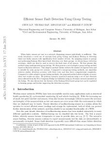
Figure 1: Semiautonomous P92 Tecnam.
that are supposed to provide an estimation of the sensor measurement. Several types of estimators can be found in the literature, such as Kalman Filters [17], Unscented Kalman Filters [18], Extended Kalman Filters [19], FIR filter estimator [20], and neural networks adaptive and nonadaptive [21, 22]. Specifically, in this effort, a nonautoregressive model [23–25] has been used. The model is essentially a nonlinear time series model, also known as nonlinear regression [26] modelled as follows: y k = f NR X k + ε k ,
1
where y k is the y k (target) estimation, X k is the final set of regressors (see Sections 4 and 5), and ε k is a modelling error. Note that the NR model does not depend on previous values ofy k ; this guarantees that the estimation is not affected by the occurrence of a fault on y k . Thus, the NR model is able to provide a reliable long-term (multistep ahead) estimation independently of the occurrence of the fault; on the contrary, an adaptive model (i.e., NARX model) estimation is influenced by the previous occurrence of a fault on k .
3. P92 Aircraft and Flight Data The proposed scheme has been validated using flight data from the semiautonomous P92 Tecnam aircraft shown in Figure 1. The P92 is a general aviation single-engine light aircraft with a classic high-wing configuration [27]. During the test flights, the aircraft was remotely controlled through a data link from a ground station. The on-board pilot was operative only during the take-off and landing phases. The nominal aircraft mass is 600 kg (1324 lb); the propulsion is provided by a Rotax 912 ULS, 74 kW (68 hp) with a two-blade fix pitch propeller, capable of providing a max cruise speed of 219 km/ h (118 kts) and an operational ceiling of 4267 (14,000 ft). A total of 8 flights were recorded for approx. 3.5 hours of flight time. The available flight data were divided into two groups, that is, training data (used for the goal of training a pseudoonline learning neural network used as AnR-based virtual sensors) and validation data (used for the assessment of the performance of the estimation scheme). Since the recorded flight data were not completely homogenous, a different number of flights were used for the robust estimation of the TAS and of the aerodynamic angles α and β. For the TAS and β analysis, two flights were used for training purposes and five flights for validation purposes. Instead, for the α analysis, two flights were used for training
International Journal of Aerospace Engineering
3 of this study. The flight parameters were recorded with a sampling time of T C = 0 1 s.
Table 1 (a) TAS training and validation flight statistics Max V(k) Mean V(k) Std V(k) (m/s) (m/s) (m/s) TR-FLIGHT-1 TR-FLIGHT-2 VAL-FLIGHT-1 VAL-FLIGHT-2 VAL-FLIGHT-3 VAL-FLIGHT-4 VAL-FLIGHT-5
37.1 35.5 37.3 37.1 33.8 34.4 38
31.3 30.5 33.4 32.1 31.1 31 32
2.6 1.1 2.8 2 0.7 1.02 1.5
Flight duration (min) 34.8 26.8 16.5 17.3 18 28.3 30.8
(b) α training and validation flight statistics Max α(k) Mean α(k) Std α(k) (deg) (deg) (deg) TR-FLIGHT-1 TR-FLIGHT-2 VAL-FLIGHT-1 VAL-FLIGHT-2 VAL-FLIGHT-3 VAL-FLIGHT-4 VAL-FLIGHT-5 VAL-FLIGHT-6
14.1 12.1 11.4 14 9.3 10.3 9.1 10.5
6.4 6.3 4.9 5.6 6.4 4.6 6.2 5.8
1.9 0.9 1.7 1.4 0.5 1.5 0.7 0.9
Flight duration (min) 34.8 26.8 16.5 17.3 18 20.3 28.3 30.8
Max β(k) Mean β(k) Std β(k) (deg) (deg) (deg)
Flight duration (min)
−0.1 0.3 −0.7 0.6 1.3 1.5 0.9
34.8 26.8 17.3 18 20.3 19.9 30.8
2.9 8.3 1.6 9.8 7.1 6.2 6.5
1.5 1.4 1.1 1.1 1.5 0.7 1.2
The true airspeed (TAS), the angle of attack (α), and the angle of sideslip (β) are all estimated as functions of a combination of measurements from all other sensors (excluding, of course, TAS, α, and β). Furthermore, the scheme does not require any information, data, or functional relationships such as the aircraft equations of motion. In other words, the approach can be applied without any loss of generality to any type of aircraft. Thus, the proposed approach can be classified as “data-driven” instead of “model-driven.” It should be clarified that in all cases, the GPS velocity was not considered. In fact, the GPS velocity and the TAS are strongly related through the relationship gps k + Vwind k = V k . Therefore, a wind gust could result as an additive fault f t of the same amplitude. Thus, TAS, α, and β are estimated as function of other measurements using the model structure described in Section 2. The initial vector of regressors X k for TAS, α, and β has been set simply selecting the signals that characterize the aircraft kinematic and dynamic response as well as considering the correlation coefficient with the target signal. The resulting regressors are X TAS0 k = φ k , ϑ k , ψ k , α k , β k , P k , Q k , R k , Nx k , Ny k , Nz k , δE K ,
(c) β training and validation flight statistics
TR-FLIGHT-1 TR-FLIGHT-2 VAL-FLIGHT-1 VAL-FLIGHT-2 VAL-FLIGHT-3 VAL-FLIGHT-4 VAL-FLIGHT-5
4. Data-Driven Modeling of the Aircraft Airspeed Velocity, Angle of Attack, and Angle of Sideslip
purposes and six flights for validation purposes. Data statistics for all the flights are shown in Tables 1(a), 1(b), and 1(c). For all flights (both training and validation), only the portion of the flight at “cruise” altitude was considered. In fact, the take-off and the initial climbing, as well as the descent and the landing, were not considered since they are associated with specific aerodynamic configurations (including, for example, the use of flaps and/or high angles-of-attack conditions). This decision was made because it was clear that not enough data were available for training the neural estimators at these conditions since only a few minutes for each flight are available. Therefore, only flight data with altitude higher than h k > 250 m were considered for the purpose
δA K , δR K , T TH k , h k , T AIR K , X α0 k = ϑ k , h k , Nx k , Ny k , Nz k , P k , Q k , R k , TAS k , β k , ψ k , δE K , δA K , δR K , T TH k , CR k ,
2
X β0 k = h k , Nx k , Ny k , Nz k , P k , Q k , R k , TAS k , α k , φ k , ϑ k , ψ k , δE K , δA K , δR K , Tr k , W k , CR k , where ϕ, ϑ, and ψ are the aircraft roll, pitch, and yaw angles, respectively; α and β are the angles of attack and sideslip, respectively; P, Q, and R are the aircraft angular rates; Nx, Ny, and Nz are the axial load factors; δE , δA , and δR are the elevator, aileron and rudder deflections, respectively; T TH is the throttle; h is the altitude; T AIR is the air temperature; T AS is the true aircraft airspeed; CR is the aircraft climbing rate; Tr is the track angle; and W is the wind direction. Note that in more general cases, additional control surface deflections could be introduced. To cope with possible nonlinearities and dynamic effects, each vector X k of potential regressors was augmented with the quadratic terms (only pure quadratic terms were added and not mixed terms), resulting in
4
International Journal of Aerospace Engineering X TAS0 k
AUG
= X TAS0 k , X 2TAS0 k ,
3
X α0 k
AUG
= X α0 k , X 2α0 k ,
4
X β0 k
AUG
= X β0 k , X 2β0 k
5
5. Regressor Selection A Matlab-based automated procedure known as Stepwise Selection [28] has been successfully used in this effort for the selection of the regressors. This scheme iteratively adds and removes variables relying on the t-statistics of the estimated regression coefficients. Starting from the initial set of regressors in (3), the final set of selected regressors provided by the Stepwise Selection procedure is given by X TAS k = α k , Q k , R k , Nx k , Nz k , T TH k , h k , ψ2 k , α2 k , δE 2 K , X α k = ϑ k , h k , Nx k , Nz k , P k , Q k , TAS k , δR K , T TH k , CR k , Nz2 , TAS2 k , T TH 2 k ,
6
regression models using the same set of regressors. In that study, it was verified that the mapping performances of the linear regression models are worse than those provided by the neural network models. This was the main motivation of the use of the neural network models in the present study. A possible motivation of this fact could be that the unknown identifying functions are not linear in the selected regressors; therefore, neural estimators work better than linear regression models.
7. Failure Modeling and Residual Whitening Failure modeling is a very important task in the overall design of fault tolerant schemes [29–31]. In the literature, several fault modeling approaches can be found, such as bias, freezing, drift, loss of accuracy, and calibration error [32]. In this effort, without any loss of generality, only two specific classes of failures have been considered, that is, step failure and ramp failures to simulate the injection of hard or soft failures. For each of these cases, the magnitude of the failure was also varied to test the fault sensitivity. Clearly, hard and soft failures provide different challenges in terms of detectability. The residual signal is defined as the difference between the sensor output and the estimate of the same signal, that is,
X β k = Nx k , Ny k , P k , Q k , R k , TAS k , φ k , δA K , δR K , Tr k ,
r k =y k −y k
8
W k , Ny2 k , TAS2 k , δR 2 K , δE 2 K Specifically, Figures 2(a)–2(c) show the variable selection process by the stepwise selection method for the three sensors. The index of the selected variables is represented by the red dots in the upper section of each figure while in the lower section the RMSE prediction error (evaluated on the training data) as function of the algorithm iteration is reported. The correlations between each regressor selected by the stepwise process and the target signal are reported, for each of the sensors, in Tables 2(a), 2(b), and 2(c):
6. Multilayer Perceptron Models The estimation model introduced in Section 2 is given by y k = f NR X k
7
For each sensor TAS, α, and β, the f NR k function was mapped through a neural network architecture. After considering different options, the neural topology selected for this study is the well-known multilayer perceptron with one hidden layer. The specific architecture for each neural approximator is shown in Table 3. Table 4 summarizes the statistical results achieved for the training flight data of the residual signals which are defined as the difference between the real values of the measured signal and its estimation r k = y k − y k . In a recent study [16], the authors compared the performance of neural network models with those of simple linear
At nominal conditions (no fault), the r k signal should theoretically approach the statistical zero. Unfortunately, this is not true in practice due to unavoidable system and measurement noise as well as estimation errors. Thus, the goals of the fault detection scheme are to detect the occurrence of the failure, as soon as possible after its occurrence, along with the minimization of false alarm rates. From a detailed statistical analysis, it became evident that the residual signal is characterized by a high level of autocorrelation caused by uncertainties at low frequencies and noise. Therefore, in its raw form, the residual signal is not a suitable tool since it contains high levels of colored noise. In fact, the residual signal should be uncorrelated for optimal FD. Therefore, a whitening filter has been designed to remove as much correlation as possible from the residual. For our purposes, it was assumed, as shown in (9), that the correlated sequence can be modeled as an autoregressive (AR) process of order N [33]: N
〠 d i ⋅ r k − i + εr k ,
9
i=1
where d i are AR parameters and εr k is white noise. The term ∑Ni=1 d i ⋅ r k − i can be considered as a one-step-ahead prediction of r k and εr k = r k − r k as the prediction error. The d i parameters were estimated through the Least Squares method to the mean squared error E2 = L−1 ∑L ε k 2 of the training data. Then, after the computing of the d i
Input variable index
International Journal of Aerospace Engineering
30 20 10 0 0
RMSE (m/s)
5
2
4
6
8
10 12 Iteration
14
16
0
20
2 1 0 0
5
10
15
20
25
Input variable index
(a) TAS variable selection process
30 20 10 0
RMSE (m/s)
0
2
4
6
8
10 12 Iteration
14
16
18
20
2 1 0 0
5
10
15
20
25
Input variable index
(b) Alpha variable selection process
30 20 10 0
RMSE (deg)
0
2
4
6
8
10 12 Iteration
14
16
18
20
0.6 0.4 0.2 0
5
10
15
(c) Beta variable selection process
Figure 2
parameters, the εr k can be simply derived as output of the linear filter: εr z = W FIR z r z ,
10
where the discrete time transfer function can be easily obtained as W FIR z = 1 − d 1 z −1 − d 2 z −2 − d 3 z −3 − −dN z −N
11
The εr z signal is therefore labeled as “whitened residual” r W k . The correct length of the whitening filter was experimentally determined by evaluating r W k for increasing values of
the filter length N, applying the Ljung-Box test [34] to verify whether the whitened residual exhibits a significant autocorrelation. Table 5 shows the final values of N selected by this design process. A comparison between the residuals before and after the whitening filtering is shown in Figures 3(a), 3(b), 4(a), 4(b), 5(a), and 5(b).
8. Design of the EWMA Filter Following the design of the whitening filter, the design of the fault detection filters was performed using tools from the statistical process control (SPC). In this context, the exponentially weighted moving average (EWMA) filter is a well-known chart used to detect the presence of small shifts
6
International Journal of Aerospace Engineering Table 2 (a) Correlation between selected regressors and TAS
α −0.9
Q
R
Nx
Nz
T TH
h
ψ2
α2
δE 2
0.05
0.13
0.73
0.2
0.35
0.24
−0.83
−0.15
0.36
(b) Correlation between selected regressors and α ϑ 0.58
h
Nx
Nz
P
Q
TAS
δR
T TH
CR
Nz2
TAS2
T TH 2
−0.005
−0.64
0.05
0.09
0.15
−0.9
−0.01
−0.4
−0.16
0.06
−0.88
−0.32
(c) Correlation between selected regressors and β Nx
Ny
P
Q
R
TAS
φ
δA
δR
Tr
W
Ny2
TAS2
δR 2
δE 2
0.1
0.9
0.1
−0.1
−0.02
0.14
0.1
0.5
0.07
0.007
0.1
−0.4
0.1
0.04
0.12
Table 3: Neural network architectures. Number of neurons in the hidden layer
Number and type of output neurons
TAS K
7 sigmoidal neurons
1 linear neuron
αK
7 sigmoidal neurons
1 linear neuron
βk
8 sigmoidal neurons
1 linear neuron
Clearly, the selection of the appropriate value of the smoothing parameter λ is critical. Larger values of λ are associated with a larger weight of the current input on the current output; conversely, smaller values of λ are associated with larger weights of all the previous input samples on the current output. The output mean and standard deviation can be computed, at stationary condition, using (14). μz = μr ,
Table 4: Training performance results. Statistics of residual signals based on TR-FLIGHT-1 and TR-FLIGHT-2. Mean (r k ) TAS K
−3
3.6 ∗ 10
−4
αK
2.1 ∗ 10
βk
−7.5 ∗ 10
−6
Std (r k )
Max (r k )
0.1129
1.9240
0.1030
1.2362
0.1992
1.8095
Table 5: Filter length and whitening filter design. N length TAS k
25
αk
55
βk
30
in process variables. The EWMA chart tracks the exponentially weighted moving average mean of all the previous samples, so that the most recent samples are weighted more heavily than the previous ones. Even though normality of the distribution is usually the basic assumption in many EWMA charts, this chart has exhibited enough robustness even with non-normally distributed data [35]. The output of the filter z k is the output of a first-order linear digital filter taking as input the whitened residual, that is, z k = 1 − λ ⋅ z k − 1 + λ ⋅ rW k 0 < λ < 1
12
σ2z = σ2r
13 λ , 2−λ
14
where μ is the mean and σ is the standard deviation. A standard commonly adopted procedure for the selection of λ was not found in the literature. In this effort, the Least Squares method [36] was used, with the goal of finding an optimized value of λ so that the sum of the sample squared errors (SSE) of the one-step prediction error ez k = r w k − z k − 1 is minimized. Figure 5 shows sample squared errors as function of λ for the z k EWMA signals produced by the r w k signals that originate from the three AD models evaluated on the training data (SSE are all shifted so that SSE 1 = 0 for all the three filters). Based on Figure 6, the tuning of the EWMA filter was performed selecting the value of λ such that the SSE is minimized. Thus, the minimum values of SSE were obtained with the values of λ in Table 6:
9. Data-Driven Threshold Setting For FD purposes, conventional approaches include the use of fixed thresholds or varying (floating) thresholds. Several studies have been conducted using both the approaches [12, 13, 37, 38], typically resulting in a trade-off between them. Fixed thresholds are easier to set since they depend on a lower number of parameters. On the other hand, fixed thresholds may not allow detection following the occurrence of small amplitude failures. The setup of floating thresholds
International Journal of Aerospace Engineering
7
Residual (m/s)
2
0
Sample autocorrelation
−2
500
0
1000
1500
2000 Time (s)
80
100 Lag
2500
3000
3500
1 0.5 0 −0.5
0
20
40
60
120
140
160
180
200
(a) TAS residual and its autocorrelation
(m/s)
2
0
Sample autocorrelation
−2
500
0
1000
1500
2000 Time (s)
80
100 Lag
2500
3000
3500
1 0.5 0 −0.5
0
20
40
60
120
140
160
180
200
Tas residual Tas whitened residual (b) TAS whitened residual and its autocorrelation
Figure 3
is, of course, more complex; however, they provide in general more robustness and better performance in terms of detectability, detection delay, and false alarm rate. Clearly, their success requires a careful design. A typical problem of floating (adaptive) thresholds can be given by an excessively fast adaptation to the failure that could result in a missed fault detection. In this effort, floating (adaptive) thresholds [39] are defined, as follows: FTUP = z + η ⋅ σ z + b, FTLOW = z − η ⋅ σ z − b,
15
where z and σ z are the mean value and the standard deviation, respectively, of the EWMA-filtered residual, both computed through a sliding window of length 1800 (180 sec), while η and b are design parameters. Once again, a standard procedure for setting η and b could not be found in the literature; therefore, an “ad hoc” sensitivity study was conducted using the training data to find the optimal values with the
goal of minimizing false alarms. Specifically, a grid search was performed over the two parameters, with η in the range 0 to 10 (with a 0.5 step increment) and b in the range 0 to 3 (with a 0.05 step increment). For each grid point, the experimental P FA was computed on the training data retaining only the couples of values (η and b) leading to an experimental P FA < 0 0001. Next, between these couples, the best was selected as the one minimizing the following index: j=
η +b σz
16
Clearly a small value for J implies a small band for the floating limiter. This is positive from a fault detection point of view. Table 7 shows the optimized values of η and b achieved applying the proposed procedure: The results of this design are summarized in Figures 7(a)– 7(c), where the experimental probability plots derived from the training data are provided.
8
International Journal of Aerospace Engineering
Residual (deg)
1
0
Sample autocorrelation
−1
0
500
1000
1500 2000 Time (s)
2500
3000
1 0.5 0 −0.5
0
20
40
60
80
100 Lag
120
140
160
180
200
Whitened residual (deg)
(a) Alpha residual and its autocorrelation
1 0 −1
Sample autocorrelation
0
500
1000
1500 2000 Time (s)
2500
3000
1 0.5 0 −0.5
0
20
40
60
80
100 Lag
120
140
160
180
200
Alpha residual Whitened alpha residual (b) Alpha whitened residual and its autocorrelation
Figure 4
In each of the Figures 7(a)–7(c), there are three lobes. The central lobe is the probability distributions of EWMA outputs, while the blue lobes are lower threshold probability distributions and the red lobes are upper threshold probability distributions. Reducing false alarms requires an intersection between the probability distribution of the EWMA filter and the probability distributions of the thresholds as small as possible. If the EWMA output does not exceed significantly the thresholds, this entails that those high false alarm rates are avoided.
10. Results Fault detection during validation tests was performed using 5 flights for the true airspeed (TAS), 6 flights for the angle of attack, and 5 flights for the angle of sideslip. The testing was conducted in simulated real time using a Simulink model. For each flight, an artificial additive fault was injected at t = 700 s with the detectors set using the values of λ, η, and b reported in Tables 6 and 7. Without any loss of generality,
two failures were considered, that is, a “fast” step and a “slow” ramp (the duration of the ramp is 10 sec, then for t > 10, the amplitude remains constant at the value for t = 10; in this case, for magnitude (or “size”) of the fault, we conventionally mean the steady state value reached by the fault signal for t = 10 s) with modeling parameters shown in Table 8. A critical parameter for a FD scheme is the number of false alarms. Clearly, a lower false alarm level implies higher robustness against system and measurement noise. The evaluation of the FD scheme was conducted in two steps; in the first step, the scheme was tested on every validation flight in a fault-free condition (without injecting any fault). This is due to the fact that false alarms are independent from the fault injection; therefore, false alarm rate was evaluated on the whole length of the flight assuming no fault. During the second step, a fault was injected to evaluate the detection delay. Tables 9(a), 9(b), and 9(c) show, for the three sensors, the number of false alarms in terms of number of samples along with the “longest continuous stay out of thresholds” time in seconds.
International Journal of Aerospace Engineering
9
Residual (deg)
2
0
Sample autocorrelation
−2
0
500
1000
1500 2000 Time (s)
2500
3000
1 0.5 0 −0.5
0
20
40
60
80
100 Lag
120
140
160
180
200
Whitened residual (deg)
(a) Beta residual and its autocorrelation
2 0 −2
Sample autocorrelation
0
500
1000
1500 2000 Time (s)
2500
3000
1 0.5 0 −0.5
0
20
40
60
80
100 Lag
120
140
160
180
200
Beta residual Whitened beta residual (b) Beta whitened residual and its autocorrelation
Figure 5
Table 6: Values of the λ parameter for an optimized design of the EWMA filter.
Tuning of the EWMA filter
0.8
λ
0.6
SSE
0.4 0.2
TAS
0.002
α
0.001
β
0.0009
0 −0.2
Table 7: Optimal design of the floating thresholds. 0
0.002
0.004
0.006
𝜆 Lamda tuning for ALPHA Lamda tuning for TAS Lamda tuning for BETA
Figure 6: EWMA tuning.
0.008
0.001
η
b
P FA
TAS
6
0.005
0.0001
Α
7
0.003
0.0001
Β
7
0.0075
0.0001
10
International Journal of Aerospace Engineering Table 8: Step magnitude and ramp slope for fault modeling.
3500 3000
Density
Step (magnitude)
10 s ramp (magnitude)
2 3 3
0.2 0.3 0.3
TAS (m/s) α (deg) β (deg)
2500 2000 1500 1000
Table 9
500 0
−5
−4
−3
−2
−1
0 Data
1
2
3
4
5 ×10⁻³
Upper threshold z(k) Lower threshold
(a) Performance for TAS: robustness against false alarms Airspeed Flight-1 Flight-2 Flight-3 Flight-4 Flight-5
(a) Threshold design for TAS: probability plot
×104 2
Flight duration False alarms (min) (number of samples) 17 17.3 18 28.3 30.8
7 0 0 0 22
Maximum stay out of thresholds (sec) 0.4 0 0 0 0.6
Density
1.5
(b) Performance for α: robustness against false alarms 1
Angle Flight duration False alarms of attack (min) (number of samples)
0.5 0
−1.5
−1
−0.5
0 Data
0.5
1
1.5 ×10⁻³
Upper threshold z(k) Lower threshold
Flight-1 Flight-2 Flight-3 Flight-4 Flight-5 Flight-6
17 17.3 18 20.3 28.3 30.8
35 8 0 34 0 56
Maximum stay out of thresholds (sec) 0.4 0.3 0 0.6 0 0.7
(b) Threshold design for α: probability density
(c) Performance for β: robustness against false alarms
1500
Angle of Flight duration False alarms sideslip (min) (number of samples)
Density
1000
Flight-1 Flight-2 Flight-3 Flight-4 Flight-5
500
0
−8
−6
−4
−2
0 Data
2
4
6
8
17.3 18 20.3 19.9 30.8
0 0 40 42 120
Maximum stay out of thresholds (sec) 0 0 1.5 1.6 2.2
10 ×10−3
Upper threshold z(k) Lower threshold (c) Threshold design for beta: probability density
Figure 7
Other critical indexes for assessing the performance of a FD scheme are the fault detection delay and the minimum amplitude detectable fault. These indexes are defined as follows:
(i) Fault Detection Delay. This is the time elapsed from the injection of the fault to the moment when the detector detects a “true fault.” (ii) Minimum Amplitude Detectable Fault. This is the minimum amplitude of the fault that produces the detection of a “true fault.” In this study, a fault detection is considered a “true fault” if, considering an observation period of 60 s following the failure, the fault detection thresholds are crossed for a time
International Journal of Aerospace Engineering
11
Table 10 (a) Detection delay for step and ramp TAS fault: ΔV = 2 m/s Airspeed
Step fault detection delay (sec)
Ramp fault detection delay (sec)
Flight-1 Flight-2 Flight-3 Flight-4 Flight-5
0.4 0.4 0.5 0.1 0.4
3.8 4.2 4.7 4 3.5
(b) Detection delay for step and ramp α fault: Δα = 3 deg Angle of attack Flight-1 Flight-2 Flight-3 Flight-4 Flight-5 Flight-6
Step fault detection delay (sec)
Ramp fault detection delay (sec)
0.3 0.1 0.1 0.1 0.1 0.1
4 7.1 8 8.3 6.9 7.2
(c) Detection delay for step and ramp β fault Δβ = 3 deg Angle of sideslip Flight-1 Flight-2 Flight-3 Flight-4 Flight-5
Step fault detection delay (sec)
Ramp fault detection delay (sec)
2.5 2.4 0.8 1.7 1.6
7.5 7.6 6.5 6.9 7.7
duration longer than 4 s during the observation period; otherwise, the detection is considered not reliable and the true fault is not declared. This logic implies that the minimum decision time for a fault declaration is 60 seconds. Tables 10(a), 10(b), and 10(c) show the performance for TAS, α, and β in terms of detection delay, while Figures 8(a), 8(b), 9(a), 9(b), 10(a), and 10(b) show the threshold evolution during the injection of the fault. The minimum amplitude detectable fault was computed by incrementally decreasing the amplitude of the fault injected until it was no longer possible to declare a “true fault” within the predefined observation period. The results for the minimum amplitude detectable faults are shown in Table 11: Tables 12(a), 12(b), and 12(c) summarize the performance of the FD scheme with the minimum amplitude detectable along with the associated fault detection delay.
11. Comparison between Adaptive- and FixedThreshold Approaches As discussed in the literature, a very interesting area of research is the performance comparison in terms of specific
FD parameters between “fixed” and “adaptive” thresholds. Considering the fixed-threshold computation approach discussed in [37] as baseline, in this study, the comparison was performance using the same training and validation data for both approaches, reporting the performance in terms of false alarms and detection delay. For the purpose of being completely objective and conducting a fair comparison, fixed thresholds have been computed starting from the residual signals using the same neural estimators and the same whitening filters to obtain a whitened residual. The difference between the two approaches starts after the EWMA filtering (designed with the same λ parameters). In fact, for the fixedthreshold approach, the EWMA output was processed to find optimized values for upper and lower limits. In fact, during the training, the UCL and LCL were derived from data depending on the desired probability of false alarm P FA , where the P FA is defined as the probability that z k exceeds the detection thresholds in a fault-free condition. Defining F z as the experimental cumulative PDF of z k , the fault detection thresholds are defined as follows: UCL = min z F z ≥ 1 − P FA , LCL = max z F z ≤ P FA
17
P FA = 0 0001 was set the same way in both approaches. Also, the validation tests were conducted on the same flights used in Section 10, using the same fault amplitude and the same injection time for the failure. Tables 13, 14, and 15 show validation results in terms of false alarms and detection delay: As far as soft failures are concerned, the detection delay analysis was performed using the minimum amplitude detectable fault used in Section 10 and reported in Table 11. The achieved results are shown in Tables 15(a), 15(b), and 15(c): Analyzing the results, it is evident that detecting fault featuring adaptive limiters could save from 0% to 50% of the time, with the same false alarm rate in the case of hard failures. Substantially different results were achieved when comparing the two approaches in the case of soft failures. In fact, adaptive thresholds allow a much lower detection delay versus fixed thresholds (up to a ratio of 1 : 30). In some cases, the occurrence of a soft failure was not even detected using fixed thresholds. Note: the study presented in this paper is specifically focused on the design of experimental FD filters. Therefore, the problem of fault isolation is not considered at all in the study. Indeed, if the fault signature matrix for the residuals for TAS, α, and β are computed, it can be immediately seen that the three faults are not strongly isolable since each residual depends on TAS, α, and β. Different approaches can be used to deal with the fault isolation problem, such as (1) to perform a fault sensitivity analysis to investigate whether the fault has a different effect on the amplitudes of three residuals and then exploit this information for discriminating the faulty signal.
International Journal of Aerospace Engineering 0.02
0.02
0.015
0.015
0.01
0.01
0.005
0.005 z(k)
z(k)
12
0
0
−0.005
−0.005
−0.01
−0.01
−0.015
−0.015
−0.02 680
685
690
695
700 705 Time (s)
710
715
−0.02 680
720
EWMA output Upper threshold Lower threshold
685
690
695
700 705 Time (s)
710
715
720
715
720
715
720
EWMA output Upper threshold Lower threshold
(a) TAS, zoom on fault detection, step fault
(b) TAS, zoom on fault detection, ramp fault
at time 700 s injected in Flight-1
at time 700 s injected in Flight-1
0.02
0.02
0.015
0.015
0.01
0.01
0.005
0.005 z(k)
z(k)
Figure 8
0
0
−0.005
−0.005
−0.01
−0.01
−0.015
−0.015
−0.02 680
685
690
695
700 705 Time (s)
710
715
−0.02 680
720
EWMA output Upper threshold Lower threshold
685
690
695
700 705 Time (s)
710
EWMA output Upper threshold Lower threshold
(a) α, zoom on fault detection, step fault
(b) α, zoom on fault detection, ramp fault
at time 700 s injected in Flight-1
at time 700 s injected in Flight-1
0.02
0.02
0.015
0.015
0.01
0.01
0.005
0.005 z(k)
z(k)
Figure 9
0 −0.005
0 −0.005
−0.01
−0.01
−0.015
−0.015
−0.02 680
685
690
695
700 705 Time (s)
710
715
720
EWMA output Upper threshold Lower threshold
−0.02 680
685
690
695
700 705 Time (s)
710
EWMA output Upper threshold Lower threshold
(a) β, zoom on fault detection, step fault
(b) β, zoom on fault detection, step fault
at time 700 s injected in Flight-1
at time 700 s injected in Flight-1
Figure 10
International Journal of Aerospace Engineering
13
Table 11: Minimum amplitude detectable faults.
Table 13
Step (magnitude)
10 s ramp (magnitude)
0.7 0.9 1.3
0.07 0.1 0.13
TAS (m/s) α (deg) β (deg)
Table 12 (a) Detection delay for step and ramp TAS fault Airspeed
Step fault detection delay (sec)
Ramp fault detection delay (sec)
Flight-1 Flight-2 Flight-3 Flight-4 Flight-5
3.7 1.9 10.2 1.9 1.4
15.4 10.1 11.3 9.4 13.8
(a) Comparison between fixed-threshold and adaptive-threshold false alarms for TAS Flight TAS duration (min) FL-1 FL-2 FL-3 FL-4 FL-5
Step fault detection delay (sec)
Ramp fault detection delay (sec)
15.5 2.8 10.4 6.2 5.5 5.7
15 8.8 10.8 10.6 9.6 18.2
Flight-1 Flight-2 Flight-3 Flight-4 Flight-5 Flight-6
α
FL-1 FL-2 FL-3 FL-4 FL-5 FL-6
Step fault detection delay (sec)
Ramp fault detection delay (sec)
17.3 13.1 15 7.6 9.8
18.3 18.6 25.5 13.3 16.4
Flight-1 Flight-2 Flight-3 Flight-4 Flight-5
(2) to exclude, a priori, from the set of regressors the reaming two signals (for instance the regressor set used for approximating the TAS signal does not include the α and β signals). In this case, we achieve, by construction, experimental models that produce a strong isolable failure signature matrix. Interested readers are referred to the recent paper by the authors in [16] where this last approach has been applied.
12. Conclusions The goal of this study was the design of a robust adaptive threshold scheme able to deal with failures involving air data
False alarms (num. of samples) (fixed)
Max stay out of thresholds (sec) (fixed)
7 0 0 0 22
0.4 0 0 0 0.6
5 2 0 3 18
0.3 0.2 0 0.2 0.5
Flight duration (min)
False alarms (num. of samples) (adapt)
Max stay out of thresholds (sec) (adapt)
False alarms (num. of samples) (fixed)
Max stay out of thresholds (sec) (fixed)
17 17.3 18 20.3 28.3 30.8
35 8 0 34 0 56
0.4 0.3 0 0.6 0 0.7
40 12 2 40 5 60
0.7 0.4 0.2 0.5 0.5 1.2
(c) Comparison between fixed-thresholds and adaptive false alarms delay for β
(c) Detection delay for step and ramp β fault Angle of sideslip
Max stay out of thresholds (sec) (adaptive)
(b) Comparison between fixed-threshold and adaptive false alarms delay for α
(b) Detection delay for step and ramp α fault Angle of attack
17 17.3 18 28.3 30.8
False alarms (num. of samples) (adaptive)
β
FL-1 FL-2 FL-3 FL-4 FL-5
False Max stay False alarms out of alarms Flight duration (num. of thresholds (num. of samples) (sec) samples) (min) (fixed) (adapt) (adapt) 17.3 18 20.3 19.9 30.8
0 0 40 42 120
0 0 1.5 1.6 2.2
5 4 45 46 80
Max stay out of thresholds (sec) (fixed) 0.2 .01 1.3 1.2 0.5
sensors. A completely data-driven approach for the design and the tuning of the FD schemes for true airspeed, angleof-attack, and angle-of-sideslip sensors of an aircraft has been proposed. It has been shown that, through the use of this scheme, it is possible to improve significantly the robustness in terms of false alarms and failure detection delay. The data-driven design philosophy was used in many parts of the overall FD procedure that is in the regressor selection phase for the considered sensors, in the design of the withering and EWMA filters as long as for the computation of detection thresholds. Validation studies based on actual flight data
14
International Journal of Aerospace Engineering Table 14
Table 15
(a) Comparison between fixed-threshold and adaptive-threshold detection delay for TAS
(a) Comparison between fixed-threshold and adaptive-threshold detection delay for TAS: soft failures
TAS
Step fault detection delay (adaptive)
Ramp fault detection delay (adaptive)
Step fault detection delay (fixed)
Ramp fault detection delay (fixed)
FL-1 FL-2 FL-3 FL-4 FL-5
0.4 0.4 0.5 0.1 0.4
3.8 4.2 4.7 4 3.5
0.7 0.7 0.8 0.7 0.8
4.8 5.7 6 6 5.6
(b) Comparison between fixed-threshold and adaptive-threshold detection delay for α
α FL-1 FL-2 FL-3 FL-4 FL-5 FL-6
Step fault detection delay (adaptive)
Ramp fault detection delay (adaptive)
Step fault detection delay (fixed)
Ramp fault detection delay (fixed)
0.3 0.1 0.1 0.1 0.1 0.1
4.0 7.1 8.0 8.3 6.9 7.2
3.6 1.6 0.6 1.8 1.2 1.1
9.3 7.2 5.5 7.4 6.8 6
(c) Comparison between fixed-threshold and adaptive-threshold detection delay for β
β FL-1 FL-2 FL-3 FL-4 FL-5
Step fault detection delay (adaptive)
Ramp fault detection delay (adaptive)
Step fault detection delay (fixed)
Ramp fault detection delay (fixed)
2.5 2.4 0.8 1.7 1.6
7.5 7.6 6.5 6.9 7.7
3 3.6 4.4 6.5 3.5
9 9 10 6.8 10
have shown good overall performance in the presence of hard and soft failures and the possibility to detect very small faults. Additionally, a comparison with a fixed-threshold approach was performed. The results of the comparison revealed that for hard failures, there is a limited difference between the approaches. In contrast, a different trend has been observed in the case of soft failures. Specifically, a significant detection delay has been observed in the case of fixed thresholds, leading also to the “no detection at all” situation in some cases. The capabilities of this data-driven FD approach coupled with the flexibility of the adaptive threshold provided by the floating limiters have proven to be substantially better than fixed-threshold methods in terms of FD performance. This last aspect makes the proposed scheme appealing for the
TAS
Step fault detection delay (adaptive)
Ramp fault detection delay (adaptive)
Step fault detection delay (fixed)
Ramp fault detection delay (fixed)
FL-1 FL-2 FL-3 FL-4 FL-5
3.7 1.9 10.2 1.9 1.4
15.4 10.1 11.3 9.4 13.8
7.6 15.3 31.5 16.3 27.8
19.4 19.2 30 17 28
(b) Comparison between fixed-threshold and adaptive-threshold detection delay for α: soft failures
α FL-1 FL-2 FL-3 FL-4 FL-5 FL-6
Step fault detection delay (adaptive)
Ramp fault detection delay (adaptive)
Step fault detection delay (fixed)
Ramp fault detection delay (fixed)
15.5 2.8 10.4 6.2 5.5 5.7
15 8.8 10.8 10.6 9.6 18.2
Not detected 86.2 10.7 41.2 Not detected 26.7
40.9 85.6 12.6 40.8 51.4 26
(c) Comparison between fixed-threshold and adaptive-threshold detection delay for β: soft failures
β FL-1 FL-2 FL-3 FL-4 FL-5
Step fault detection delay (adaptive)
Ramp fault detection delay (adaptive)
Step fault detection delay (fixed)
Ramp fault detection delay (fixed)
17.3 13.1 15 7.6 9.8
18.3 18.6 25.5 13.3 16.4
19 21 43.8 5.9 46.7
20 23 48.1 11.2 42.8
application to a variety of sensor failures for systems where physical redundancy in the sensors is not available.
Data Availability Research data are not made freely available due to a confidentiality agreement between the authors and Tecnam.
Conflicts of Interest The authors Fabio Balzano, Mario L. Fravolini, Marcello R. Napolitano, Stéphane D’Urso, Michele Crispoltoni, and Giuseppe del Core declare that there is no conflict of interest regarding the publication of this paper.
International Journal of Aerospace Engineering
References [1] R. P. Collinson, Introduction to Avionics Systems, Springer Science and Business, 2013. [2] Bureau d’Enquetes et d’Analyses pour la securite de l’aviation civile, “Re-port 3: on the accident on 1 June 2009 to the Airbus A330–203 registered F-GZCP operated by Air France flight AF 447 Rio de Janeiro–Paris, France,” https://www.bea.aero/ docspa/2009/f-cp090601.en/pdf/f-cp090601.en.pdf. [3] J. Levine, J.X-31’s loss, NASA X-Press, 2004, http://www.nasa. gov/centers/dryden/news/X-Press/stories/2004/013004/ new_x31.html. [4] J. T. McKenna, “Blocked static ports eyed in Aeroperu 757 crash,” Aviation Week & Space Technology, vol. 145, no. 20, p. 76, 1996. [5] Dirección General de Aeronáutica Civil (Dominican Republic), “Reporte final accidente aereo Birgenair, vuelo ALW301,” 1996, http://www.fss.aero/accident-reports/. [6] Bureau d'Enquêtes et d'Analyses pour la Sécurité de l'Aviation Civile, “Report of the accident on 27 November 2008 off the coast of Canet-Plage (66) to the Airbus A320-232 registered D-AXLA operated by XL Airways Germany,” https://www. bea.aero/. [7] E. Dubrova, Fault-Tolerant Design, Springer, Berlin, 2013. [8] P. M. Frank, “Fault diagnosis in dynamic systems using analytical and knowledge-based redundancy: a survey of some new results,” Automatica, vol. 26, no. 3, pp. 459–474, 1990. [9] R. C. Swischuk and D. L. Allaire, “A machine learning approach to aircraft sensor error detection and correction,” in Proceeding of the 2018 AIAA/ASCE/AHS/ASC Structures, Structural Dynamics, and Materials Conference, p. 1164, Kissimmee, FL, USA, 2018. [10] S. X. Ding, Data-Driven Design of Fault Diagnosis and FaultTolerant Control Systems, Springer, 2014. [11] S. Simani, C. Fantuzzi, and R. J. Patton, Model-Based Fault Diagnosis, in Dynamic Systems Using Identification Techniques, Springer-Verlag, 2002. [12] N. Talebi, M. A. Sadrnia, and A. Darabi, “Robust fault detection of wind energy conversion systems based on dynamic neural networks,” Computational intelligence and neuroscience, vol. 2014, Article ID 580972, 13 pages, 2014. [13] J. Qi, X. Zhao, Z. Jiang, and J. Han, “An adaptive threshold neural-network scheme for rotorcraft UAV sensor failure diagnosis,” in Advances in Neural Networks – ISNN 2007, D. Liu, S. Fei, Z. Hou, H. Zhang, and C. Sun, Eds., vol. 4493 of Lecture Notes in Computer Science, Springer, Berlin, Heidelberg, 2007. [14] J. M. Lucas and M. S. Saccucci, “Exponentially weighted moving average control schemes: properties and enhancements,” Technometrics, vol. 32, no. 1, pp. 1–12, 1990. [15] J. S. Hunter, “The exponentially weighted moving average,” Journal of Quality Technology, vol. 18, no. 4, pp. 203–210, 2018. [16] M. L. Fravolini, M. R. Napolitano, G. D. Core, and U. Papa, “Experimental interval models for the robust fault detection of aircraft air data sensors,” Control Engineering Practice, vol. 78, pp. 196–212, 2018. [17] Q. Li, R. Li, K. Ji, and W. Dai, “Kalman filter and its application,” in 2015 8th International Conference on Intelligent Networks and Intelligent Systems (ICINIS), pp. 74–77, Tianjin, China, 2015.
15 [18] E. A. Wan and R. Van Der Merwe, “The unscented Kalman filter for nonlinear estimation,” in Proceedings of the IEEE 2000 Adaptive Systems for Signal Processing, Communications, and Control Symposium (Cat. No.00EX373), Lake Louise, Alberta, Canada, 2000. [19] F. Keisuke, “Extended Kalman filter,” Reference Manual, 2013, http://www-jlc.kek.jp/2003oct/subg/offl/kaltest/doc/Reference Manual.pdf. [20] S. Zhao, F. Liu, and Y. S. Shmaliy, “Optimal FIR estimator for discrete time-variant state-space model,” in 2014 11th International Conference on Electrical Engineering, Computing Science and Automatic Control (CCE), pp. 1–5, Campeche, Mexico, 2014. [21] K. Hornik, M. Stinchcombe, and H. White, “Multilayer feedforward networks are universal approximators,” Neural Networks, vol. 2, no. 5, pp. 359–366, 1989. [22] D. Svozil, V. Kvasnicka, and J.̂. Pospichal, “Introduction to multi-layer feed-forward neural networks,” Chemometrics and Intelligent Laboratory Systems, vol. 39, no. 1, pp. 43–62, 1997. [23] N. Oliver, Nonlinear System Identification: from Classical Approaches to Neural Networks and Fuzzy Models, SpringerVerlag, 2001. [24] I. Rivals and L. Personnaz, “MLPs (mono layer polynomials and multi-layer perceptrons) for nonlinear modeling,” Journal of Machine Learning Research, vol. 3, pp. 1383–1398, 2003. [25] M. W. Gardner and S. R. Dorling, “Artificial neural networks (the multilayer perceptron)—a review of applications in the atmospheric sciences,” Atmospheric Environment, vol. 32, no. 14–15, pp. 2627–2636, 1998. [26] J. A. Farrell and M. M. Polycarpou, Adaptive Approximation Based Control: Unifying Neural, Fuzzy and Traditional Adaptive Approximation Approaches, Wiley, 2006. [27] https://www.tecnam.com/it/aircraft/p92-eaglet-adv-ul/. [28] N. R. Draper and H. Smith, Applied Regression Analysis, Wiley-Interscience, Hoboken, NY, USA, 1998. [29] N. Nyberg, “A general framework for fault diagnosis based on statistical hypothesis testing,” in Proceedings of the 12th International Workshop on Principles of Diagnosis, pp. 135–142, Sansicario, Italy, 2001. [30] J. Gertler, “Analytical redundancy methods in fault detection and isolation; survey and synthesis,” in Proceedings of the IFAC Fault Detection, Supervision and Safety for Technical Processes, pp. 9–21, Baden, Germany, 1991. [31] J. Chen and R. J. Patton, Robust Model-Based Fault Diagnosis for Dynamic Systems, Kluwer, 1999. [32] H. Alwi, C. Edwards, and C. P. Tan, “Fault tolerant control and fault detection and isolation,” in Fault Detection and FaultTolerant Control Using Sliding Modes. Advances in Industrial Control, Springer, 2011. [33] D. C. Montgomery and C. M. Mastrangelo, “Some statistical process control methods for autocorrelated data,” Journal of Quality Technology, vol. 23, no. 3, pp. 179–193, 2018. [34] G. M. Ljung and G. E. P. Box, “On a measure of lack of fit in time series models,” Biometrika, vol. 65, no. 2, pp. 297–303, 1978. [35] N. Ye, S. Vilbert, and Q. Chen, “Computer intrusion detection through EWMA for autocorrelated and uncorrelated data,” IEEE Transactions on Reliability, vol. 52, no. 1, pp. 75–82, 2003.
16 [36] J. S. Oakland, Statistical Process Control, ButterworthHeinemann, Burlington, MA, USA, 2007. [37] M. L. Fravolini, G. del Core, U. Papa, P. Valigi, and M. R. Napolitano, “Data-driven schemes for robust fault detection of air data system sensors,” IEEE Transactions on Control Systems Technology, no. 99, pp. 1–15, 2017. [38] S. A. Raka and C. Combastel, “Fault detection based on robust adaptive thresholds: a dynamic interval approach,” Annual Reviews in Control, vol. 37, no. 1, pp. 119–128, 2013. [39] M. G. Perhinschi, M. R. Napolitano, G. Campa, B. Seanor, J. Burken, and R. Larson, “An adaptive threshold approach for the design of an actuator failure detection and identification scheme,” IEEE Transactions on Control Systems Technology, vol. 14, no. 3, pp. 519–525, 2006.
International Journal of Aerospace Engineering
International Journal of
Advances in
Rotating Machinery
Engineering Journal of
Hindawi www.hindawi.com
Volume 2018
The Scientific World Journal Hindawi Publishing Corporation http://www.hindawi.com www.hindawi.com
Volume 2018 2013
Multimedia
Journal of
Sensors Hindawi www.hindawi.com
Volume 2018
Hindawi www.hindawi.com
Volume 2018
Hindawi www.hindawi.com
Volume 2018
Journal of
Control Science and Engineering
Advances in
Civil Engineering Hindawi www.hindawi.com
Hindawi www.hindawi.com
Volume 2018
Volume 2018
Submit your manuscripts at www.hindawi.com Journal of
Journal of
Electrical and Computer Engineering
Robotics Hindawi www.hindawi.com
Hindawi www.hindawi.com
Volume 2018
Volume 2018
VLSI Design Advances in OptoElectronics International Journal of
Navigation and Observation Hindawi www.hindawi.com
Volume 2018
Hindawi www.hindawi.com
Hindawi www.hindawi.com
Chemical Engineering Hindawi www.hindawi.com
Volume 2018
Volume 2018
Active and Passive Electronic Components
Antennas and Propagation Hindawi www.hindawi.com
Aerospace Engineering
Hindawi www.hindawi.com
Volume 2018
Hindawi www.hindawi.com
Volume 2018
Volume 2018
International Journal of
International Journal of
International Journal of
Modelling & Simulation in Engineering
Volume 2018
Hindawi www.hindawi.com
Volume 2018
Shock and Vibration Hindawi www.hindawi.com
Volume 2018
Advances in
Acoustics and Vibration Hindawi www.hindawi.com
Volume 2018