3.2.4 Critical points and locations of elementary domains . ..... object and theoretical predictions can be immediately verified by the easily affordable new experiments. ... Unfortunately, these names are already associated with narrower fields of.
/hepth-0501235 ITEP-TH-02/05
Algebraic Geometry of Discrete Dynamics The case of one variable V.Dolotin and A.Morozov ITEP, Moscow and JINR, Dubna; Russia
arXiv:hep-th/0501235v2 29 Mar 2005
ABSTRACT We argue that discrete dynamics has natural links to the theory of analytic functions. Most important, bifurcations and chaotic dynamical properties are related to intersections of algebraic varieties. This paves the way to identification of boundaries of Mandelbrot sets with discriminant varieties in moduli spaces, which are the central objects in the worlds of chaos and order (integrability) respectively. To understand and exploit this relation one needs first to develop the theory of discrete dynamics as a solid branch of algebraic geometry, which so far did not pay enough attention to iterated maps. The basic object to study in this context is Julia sheaf over the universal Mandelbrot set. The base has a charateristic combinatorial structure, which can be revealed by resultant analysis and represented by a basic graph. Sections (Julia sets) are contractions of a unit disc, related to the action of Abelian Z group on the unit circle. Their singularities (bifurcations) are located at the points of the universal discriminant variety.
1
Contents 1 Introduction 2 Notions and notation 2.1 Objects, associated with the space X . 2.2 Objects, associated with the space M 2.3 Combinatorial objects . . . . . . . . . 2.4 Relations between the notions . . . . .
4 . . . .
. . . .
. . . .
. . . .
. . . .
. . . .
. . . .
. . . .
. . . .
. . . .
. . . .
. . . .
. . . .
. . . .
. . . .
. . . .
. . . .
. . . .
. . . .
. . . .
. . . .
. . . .
3 Summary 3.1 Orbits and grand orbits . . . . . . . . . . . . . . . . . . . . . . . . . . . . . . 3.2 Mandelbrot sets . . . . . . . . . . . . . . . . . . . . . . . . . . . . . . . . . . . 3.2.1 Forest structure . . . . . . . . . . . . . . . . . . . . . . . . . . . . . . . 3.2.2 Relation to resultants and discriminants . . . . . . . . . . . . . . . . . 3.2.3 Relation to stability domains . . . . . . . . . . . . . . . . . . . . . . . 3.2.4 Critical points and locations of elementary domains . . . . . . . . . . 3.2.5 Perturbation theory and approximate self-similarity of Mandelbrot set 3.2.6 Trails in the forest . . . . . . . . . . . . . . . . . . . . . . . . . . . . . 3.3 Sheaf of Julia sets over moduli space . . . . . . . . . . . . . . . . . . . . . . . 4 Fragments of theory 4.1 Orbits and reduction theory of iterated maps . . . . . . . . . . . . . . 4.2 Bifurcations and discriminants: from real to complex . . . . . . . . . . 4.3 Discriminants and resultants for iterated maps . . . . . . . . . . . . . 4.4 Period-doubling and beyond . . . . . . . . . . . . . . . . . . . . . . . . 4.5 Stability and Mandelbrot set . . . . . . . . . . . . . . . . . . . . . . . 4.6 Towards the theory of Julia sets . . . . . . . . . . . . . . . . . . . . . 4.6.1 Grand orbits and algebraic Julia sets . . . . . . . . . . . . . . . 4.6.2 From algebraic to ordinary Julia set . . . . . . . . . . . . . . . 4.6.3 Bifurcations of Julia set . . . . . . . . . . . . . . . . . . . . . . 4.7 On discriminant analysis for grand orbits . . . . . . . . . . . . . . . . 4.7.1 Decomposition formula for Fn,s (x; f ) . . . . . . . . . . . . . . . 4.7.2 Irreducible constituents of discriminants and resultants . . . . 4.7.3 Discriminant analysis at the level (n, s) = (1, 1): basic example 4.7.4 Sector (n, s) = (1, s) . . . . . . . . . . . . . . . . . . . . . . . . 4.7.5 Sector (n, s) = (2, s) . . . . . . . . . . . . . . . . . . . . . . . . 4.7.6 Summary . . . . . . . . . . . . . . . . . . . . . . . . . . . . . . 4.7.7 On interpretation of wn,k . . . . . . . . . . . . . . . . . . . . . 4.8 Combinatorics of discriminants and resultants . . . . . . . . . . . . . . 4.9 Shapes of Julia and Mandelbrot sets . . . . . . . . . . . . . . . . . . . 4.9.1 Generalities . . . . . . . . . . . . . . . . . . . . . . . . . . . . . 4.9.2 Exact statements about 1-parametric families of polynomials of 4.9.3 Small-size approximation . . . . . . . . . . . . . . . . . . . . . 4.9.4 Comments on the case of fc (x) = xd + c . . . . . . . . . . . . 4.10 Analytic case . . . . . . . . . . . . . . . . . . . . . . . . . . . . . . . . 4.11 Discriminant variety D . . . . . . . . . . . . . . . . . . . . . . . . . . 4.11.1 Discriminants of polynomials . . . . . . . . . . . . . . . . . . . 4.11.2 Discriminant variety in entire M . . . . . . . . . . . . . . . . . 4.12 Discussion . . . . . . . . . . . . . . . . . . . . . . . . . . . . . . . . . .
2
. . . .
. . . .
. . . .
. . . .
. . . .
. . . .
. . . .
. . . .
. . . .
8 . 8 . 11 . 14 . 15
. . . . . . . . . . .
. . . . . . . . .
. . . . . . . . .
. . . . . . . . .
. . . . . . . . .
. . . . . . . . .
. . . . . . . . .
. . . . . . . . .
. . . . . . . . .
. . . . . . . . .
17 17 17 17 18 19 19 19 20 20
. . . . . . . . . . . . . . . . . . . . . . . . . . . .
. . . . . . . . . . . . . . . . . . . . . . . . . . . .
. . . . . . . . . . . . . . . . . . . . . . . . . . . .
. . . . . . . . . . . . . . . . . . . . . . . . . . . .
. . . . . . . . . . . . . . . . . . . . . . . . . . . .
. . . . . . . . . . . . . . . . . . . . . . . . . . . .
. . . . . . . . . . . . . . . . . . . . . . . . . . . .
. . . . . . . . . . . . . . . . . . . . . . . . . . . .
. . . . . . . . . . . . . . . . . . . . . . . . . . . .
23 23 24 25 26 27 28 28 28 29 30 30 30 31 32 33 34 37 42 43 43 43 44 45 46 48 48 49 50
. . . . . . . . . .
. . . . . . . . . . . . . . . . . . . . . . . . . . . . . . . . . . . . . . . . . . . . . . . . . . . . . . . . . . . . . . . . . . . . . . . . . . . . . . . . . . . . . . . . . . . . . . . . . . . . power-d . . . . . . . . . . . . . . . . . . . . . . . . . . . . . . . . . . .
. . . . . . . . . . . . . . . . . . . . . . . . . . . .
5 Map f (x) = x2 + c: from standard example to general conclusions 52 5.1 Map f (x) = x2 + c. Roots and orbits, real and complex . . . . . . . . . . . . . . . . . . . . . . . 52 5.1.1 Orbits of order one (fixed points) . . . . . . . . . . . . . . . . . . . . . . . . . . . . . . . . 52 5.1.2 Orbits of order two . . . . . . . . . . . . . . . . . . . . . . . . . . . . . . . . . . . . . . . . 53 5.1.3 Orbits of order three . . . . . . . . . . . . . . . . . . . . . . . . . . . . . . . . . . . . . . . 54 5.1.4 Orbits of order four . . . . . . . . . . . . . . . . . . . . . . . . . . . . . . . . . . . . . . . 55 5.1.5 Orbits of order five . . . . . . . . . . . . . . . . . . . . . . . . . . . . . . . . . . . . . . . . 56 5.1.6 Orbits of order six . . . . . . . . . . . . . . . . . . . . . . . . . . . . . . . . . . . . . . . . 57 5.2 Mandelbrot set for the family fc (x) = x2 + c . . . . . . . . . . . . . . . . . . . . . . . . . . . . . 58 5.3 Map f (x) = x2 + c. Julia sets, stability and preorbits . . . . . . . . . . . . . . . . . . . . . . . . 58 5.4 Map f (x) = x2 + c. Bifurcations of Julia set and Mandelbrot sets, primary and secondary . . . 67 5.5 Conclusions about the structure of the ”sheaf” of Julia sets over moduli space (of Julia sets and their dependence on 6 Other examples 6.1 Equivalent maps . . . . . . . . . . . . . . . . . . . 6.2 Linear maps . . . . . . . . . . . . . . . . . . . . . 6.2.1 The family of maps fαβ = α + βx . . . . . 6.2.2 Multidimensional case . . . . . . . . . . . . 6.3 Quadratic maps . . . . . . . . . . . . . . . . . . . . 6.3.1 Diffeomorphic maps . . . . . . . . . . . . . 6.3.2 Map f = x2 + c . . . . . . . . . . . . . . . . 6.3.3 Map fγβ0 = γx2 + βx = γx2 + (b + 1)x . . 6.3.4 Generic quadratic map and f = x2 + px + q 6.3.5 Families as sections . . . . . . . . . . . . . 6.4 Cubic maps . . . . . . . . . . . . . . . . . . . . . . 6.4.1 Map fp,q (x) = x3 + px + q . . . . . . . . . 6.4.2 Map fc = x3 + c . . . . . . . . . . . . . . . 6.4.3 Map fc (x) = cx3 + x2 . . . . . . . . . . . . 6.4.4 fγ = x3 + γx2 . . . . . . . . . . . . . . . . . 6.4.5 Map fa;c = ax3 + (1 − a)x2 + c . . . . . . 6.5 Quartic maps . . . . . . . . . . . . . . . . . . . . . 6.5.1 Map fc = x4 + c . . . . . . . . . . . . . . . 6.6 Maps fd;c (x) = xd + c . . . . . . . . . . . . . . . . P 6.7 Generic maps of degree d, f (x) = di=0 αi xi . . .
. . . . . . . . . . . . . . . . . . . .
. . . . . . . . . . . . . . . . . . . .
. . . . . . . . . . . . . . . . . . . .
. . . . . . . . . . . . . . . . . . . .
. . . . . . . . . . . . . . . . . . . .
. . . . . . . . . . . . . . . . . . . .
. . . . . . . . . . . . . . . . . . . .
. . . . . . . . . . . . . . . . . . . .
. . . . . . . . . . . . . . . . . . . .
. . . . . . . . . . . . . . . . . . . .
. . . . . . . . . . . . . . . . . . . .
. . . . . . . . . . . . . . . . . . . .
. . . . . . . . . . . . . . . . . . . .
. . . . . . . . . . . . . . . . . . . .
. . . . . . . . . . . . . . . . . . . .
. . . . . . . . . . . . . . . . . . . .
. . . . . . . . . . . . . . . . . . . .
. . . . . . . . . . . . . . . . . . . .
. . . . . . . . . . . . . . . . . . . .
. . . . . . . . . . . . . . . . . . . .
. . . . . . . . . . . . . . . . . . . .
. . . . . . . . . . . . . . . . . . . .
. . . . . . . . . . . . . . . . . . . .
. . . . . . . . . . . . . . . . . . . .
. . . . . . . . . . . . . . . . . . . .
. . . . . . . . . . . . . . . . . . . .
78 78 78 78 79 79 80 81 82 83 84 86 87 91 94 97 100 103 103 105 108
7 Conclusion
110
8 Acknowledgements
112
3
1
Introduction
This paper is devoted to the structure of Mandelbrot set – a remarkable and important personage of the modern theoretical physics, related to chaos and fractals and simultaneously to analytical functions, Riemann surfaces and phase transitions. This makes Mandelbrot set one of the bridges connecting the worlds of chaos and order (integrability). At the same time the Mandelbrot set is a very simple object, allowing detailed experimental investigation with the help of the easily available computer programs and profound theoretical analysis with the help of undergraduate-level mathematics. This makes Mandelbrot set a wonderful subject of physical investigation: one needs to look for theoretical explanations of experimentally observable properties of the object and theoretical predictions can be immediately verified by the easily affordable new experiments. In this paper we just lift the cover of Pandora box: if interested, the reader can easily continue along any of the research lines, which are mentioned below, or, digging a little deeper into the experimental data, find and resolve a lot of new puzzles, – all this without any special mathematical background. Remarkably, when thinking about this simple subject one appears in the close vicinity of modern problems of the ”high theory”: the subject is not only simple, it is also deep. Mandelbrot set shows up in the study of trajectories (world lines) behavior change under a change of the laws of motion. Generally speaking, trajectory depends on two types of data: on the motion law (e.g. on the choice of the Hamiltonian) and on the initial (boundary) conditions. The pattern of motion (the phase portrait of the system) can be rather sophisticated: trajectories can tend to fixed points, to limit cycles, to strange attractors and go away from the similar types of structures, some trajectories can go to infinity; trajectories can wrap around each other, knot and unknot etc. In this paper the information about the phase portrait will be collected in Julia sets, the structure of these sets encodes information about the world lines dependence on the initial conditions. If the law of motion is changed, the phase portrait = Julia set is also deformed. These changes can be pure quantitative (due to the variations of the shape of trajectories, of foci and limit cycles positions) and – sometime – qualitative (looking as reshuffling of the phase portrait, creation or elimination of the fixed points, cycles, attractors etc). The Mandelbrot set or its boundary, to be precise, is exactly the set of all the points in the laws-of-motion space (say in the space of Hamiltonians) where the qualitative reshufflings (phase transitions) take place. Therefore the problems about the Mandelbrot set (or, better, about the set of the phase portraits, associated with various laws of motion, i.e. about the ”sheaf of Julia sets over the Mandelbrot set”) are the typical problems about the structure of the space of theories (laws of motion), about what changes and what remains intact in transition from one theory to another. In other words, these are typical problems from the string theory1 – the science which studies the various sets of similar physical models and studies the change of the experimentally measurable characteristics with the change of the model. Moreover, in the case of the Mandelbrot set one can immediately address the problems from a difficult branch of string theory, which nowadays attracts a good deal of attention, – from landscape theory, which wonders how often is a given property encountered in the given set of models (i.e. associates with the various physical quantities, say, scattering amplitudes or mass spectra, the measures on the space of theories, which specify how frequent are the amplitudes of the given type or masses of the given values in the models of the given type). One of the lessons, taught by the study of Mandelbrot sets, is that even if the phase transitions are relatively rare in the space of theories, the phase transition points are not distributed in a uniform way, they tend to condense and form clusters of higher dimensions, up to codimension one, which actually separate – the naively un-separated – domains in the space of theories and make this space disconnected. This lesson is important for the theory of effective actions, for problems of their analytical continuations, for construction of special functions (τ -functions) which can describe these effective actions, and for many other – conceptual and practical – applications of string theory. Dynamics, essential for this type of applications of Mandelbrot-set theory, is not obligatory the ordinary dynamics in physical space-time, often the relevant one is dynamics in the space of coupling constants, i.e. the (generalized) renormalization group flow. In this paper we restrict consideration to discrete dynamics of a single variable. This restriction preserves most essential properties of the subject, but drastically simplifies computer simulations and mathematical formalism (for example, substitutes the study of arbitrary analytic functions by that of polynomials or the study of arbitrary spectral surfaces of arbitrary dimension by that of the ordinary Riemann surfaces). However, 1 As often happens, the name is pure historical and refers to a concrete set of models, which were first successfully approached from such direction. Better name could be ”the theory of theories” (sometime ”abbreviated” to pretentious ”theory of everything”) or, most adequate, ”generic quantum field theory”. Unfortunately, these names are already associated with narrower fields of research, where accents are put on somewhat different issues.
4
throughout the text we use every chance to show directions of possible generalizations. Getting rid of the infinitedimensional algebras (loop algebras), which would be unavoidable in considerations of continuous dynamics, we concentrate instead on another infinity: unification of various one-dimensional Mandelbrot sets, shown in numerous pictures below and associated with particular 1-dimensional families of evolution operators, into a total (infinite-dimensional) universal Mandelbrot set, shown symbolically in Fig.46 at the very end of the paper. Understanding the structure of this set (which has a pure cathegorial nature of the universal discriminant variety) can be one of the intermediate targets of the theory. The notions of discriminant and resultant are assumed familiar from the courses on general algebra and are actively used already in the Introduction. Still, if necessary, all the necessary definitions and properties can be found in s.4.12 of the present paper (the section itself is devoted to generalizations from polynomials to arbitrary analytic functions). The theory of deterministic dynamical systems [1], x˙ i = β i (x),
(1)
is one of the main chapters of theoretical and mathematical physics. One of the goals of the theory is to classify the types of motion – from completely integrable to fully ergodic, – and understand their dependence on the choice of the vector field β(x) and initial conditions. Discrete dynamics, in the avatar of Poincare map, xi −→ f i (x), ∂f i j β (x), β i (f (x)) = ∂xj
(2)
naturally arises in attempts to develop such a theory and plays the principal role in computer experiments (which – in the absence of adequate theory – remain the main source of information about dynamical systems). In quantum field/string theory (QFT) the most important (but by no means unique) appearance of the problem (1) is in the role of renormalization group (RG) flow. As usual, QFT relates (1) to a problem, formulated in terms of effective actions, this time to a Callan-Symanzik equation for a function F (x, ϕ) of the coupling constants xi and additional variable ϕ (having the meaning of logarithm of background field) β i (x)
∂F ∂F + = 0. ∂xi ∂ϕ
(3)
In other contexts solutions to this equation are known as characteristics [2] of the problem (1): in the case of one variable the solution function of ϕ− s(x) or of x(s = ϕ), its ϕ dependence is induced by the action of � P is arbitrary operator exp −ϕ i β i ∂i . Until recently only simple types of motions (attraction and repulsion points) were considered in the context of RG theory, but today this restriction is no longer fashionable (see, for example, [3] for the first examples of RG with periodic behaviour and [4]-[6] for further generalizations). In this context the discrete dynamics is associated with the original Kadanoff-style formulation of renormalization group, and Callan-Symanzik equation (3) becomes a finite-difference equation.2 Bifurcations of dynamical behaviour of trajectories with the change of β(x) in (1) are associated with transitions between different branches of effective actions [7]. One of the most intriguing points here is that the theory of effective actions is actually the one of 2 This
discrete equation looks like
F± (f ◦n (x), ϕ ± n) = F± (x, ϕ)
Its generic solution is arbitrary function of any of its particular solutions. Formally, such particular solutions are given by the differences ϕ ∓ n ˆ (x), where n ˆ (x) is the ”time”, needed to reach the point x, i.e. a solution of the equation f ◦n (x0 ) = x for given f and x0 . In other words, particular solutions are formally provided by the ϕ-th image and ϕ-th preimage of f (x),
n
F± (x, ϕ) = f ◦(∓ϕ) (x)
For example, if f (x) = xc and f ◦ (x) = xc , then the generic solution to is an arbitrary function of the variable c∓ϕ log x. Consideration of the present paper provides peculiar ϕ-independent solutions (zero-modes), associated with periodic f -orbits. For example, the ”orbit δ-function” F± (x, ϕ) = Fn′ (x)δ(Fn (x))
is a solution of such type (see eq.(23) below) – a generalization of continuous-case zero-mode F (x, ϕ) = det
� ∂β � ∂x
δ(β(x)).
At least in this sense periodic f -orbits are discrete analogues of non-trivial zeroes of β-function, in continuum limit they can turn into limit cycles and strange attractors.
5
integrable systems – effective actions usually are τ -functions, RG flows are multi-directional (since the boundary of integration domain in functional integral can be varied in many different ways) and related to Whitham dynamics [8]. Obvious existence of non-trivial RG flows (describing, for example, how a fractal variety changes with the change of scale) – along with many other pieces of evidence – implies existence of a deep relation between the worlds of order and chaos (represented by τ -functions and dynamical systems respectively and related by the – yet underdeveloped – theory of effective actions). Description of effective actions (prepotentials) F (ϕ, x) in situations when (1) exhibits chaotic motion remains an important open problem. Of course, one does not expect to express such F through ordinary elementary or special functions, but we are going to claim in this paper that the adequate language can still be searched for in the framework of algebraic geometry, in which the theory of dynamical systems can be naturally embedded, at least in the discrete case. The goal of this paper is to overview the connection between the discrete dynamics of one complex variable [9], which studies the properties of the iterated map x → f (x) → f ◦2 (x) : = f (f (x)) → . . . → f ◦n (x) → . . . , (4) P and the algebraic properties of the (locally) analytic function f (x) = k ak xk , considered as an element of the (infinite-dimensional) space M of all analytic functions C → C on the complex plane C. We attribute the apparent complexity of the Julia and Mandelbrot sets, associated with the pattern of orbit bifurcations, to the properties of well defined (but not yet well-studied) algebraic subspaces in moduli space: discriminant variety D and spaces of shifted n-iterated maps M◦n Fn (x; f ) = f ◦n (x) − x.
(5)
In other words, we claim that Julia and Mandelbrot sets can be defined as objects in algebraic geometry and studied by theoretical methods, not only by computer experiments. We remind, that the boundary of Julia set ∂J(f ) for a given f is the union of all unstable periodic orbits of f in C, i.e. a subset in the union O(f ) off all periodic orbits, perhaps, complex, which, in turn, is nothing but the set of all roots of the iterated maps Fn (x; f ) for all n. The boundary of algebraic Mandelbrot set ∂M (µ) ⊂ µ ⊂ M consists of all functions f from a given family µ ⊂ M, where the stability of orbits changes. However, there is no one-to-one correspondence between Mandelbrot sets and bifurcations of Julia sets, since the latter can also occur when something happens to unstable orbits and some of such events do not necessarily involve stable orbits, controlled by the Mandelbrot set. In order to get rid of the reference to somewhat subtle notion of stability (which also involves real instead of complex-analytic constraints), we suggest to reveal the algebraic structure of Julia and Mandelbrot sets and then use it is a definition of their algebraic counterparts. It is obvious that boundaries of Mandelbrot sets are related to discriminants, ∂M = D ⊂ M and can actually be defined without reference to stability. The same is true also for Julia sets, which can be defined in terms of grand orbits of f , which characterize not only the images of points after the action of f , but also their pre-images. The bifurcations of so defined algebraic Julia sets occur at the boundary of what we call the grand Mandelbrot set, a straightforward extension of Mandelbrot set, also representable as discriminant variety. Its boundary consists of points in the space of maps (moduli space), where the structure of periodic orbits (not obligatory stable) and their pre-orbits changes. Hypothetically algebraic Julia sets coincide with the ordinary ones (at least for some appropriate choice of stability criterium). To investigate the algebraic structure of Julia and Mandelbrot sets we suggest to reformulate the problem in terms of representation theory. An analytic function as a map f : C → C defines an action of Z on C: n 7→ f ◦ . . . ◦ f . For f with | {z } n
real coefficients this action has two invariant subsets R and C − R. Often in discrete dynamics one considers only the action on R. However, some peculiar properties of this action (like period doubling, stability etc.) become transparent only if we consider it as a special case of the action of f with complex coefficients and no distinguished subsets (like R) in C. The set of periodic orbits of this action can be considered as a representation of Abelian group Z, which depends on the shape of f . One can study these representations, starting from generic representation, which corresponds to generic position of f in the space M. Other representations result from merging of the orbits of 6
generic representation, what happens when f belongs to certain discriminant subsets Dn∗ = (D ∩ Mn )∗ ⊂ M. These discriminant sets are algebraic and have grading, related to the order of the corresponding merging orbits. The boundary of Mandelbrot set ∂M (µ) for a one-parametric family of maps µ ⊂ M is related to the union of the countable family of algebraic sets of increasing degree, ∪∞ n=0 (D ∩ µ◦n ), and this results in the ”fractal” structure of Mandelbrot set. This approach allows us to introduce the notion of discriminant in the (infinitedimensional) space M of analytic functions as the inverse limit of a sequence of finite-dimensional expressions corresponding to discriminants in the spaces of polynomials with increasing degree. On the preimages of periodic orbits (on bounded grand orbits) the above Z-action is not invertible. The structure of the set of preimages of a given order k has special bifurcations which are not expressible in terms of bifurcations of periodic orbits. This implies the existence of a hierarchy of discriminant sets in the space of coefficients (secondary Mandelbrot sets). The union of secondary Mandelbrot sets for all k presumably defines all the bifurcations of Julia sets. We call this union the Grand Mandelbrot set. Mentioned above is just one of many possible ”definitions” of Julia and Mandelbrot sets [10]. Their interesting (fractal) properties look universal and not sensitive to particular way they are introduced, what clearly implies that some canonical universal structure stands behind. The claim of the present paper is that this canonical structure is algebraic and is nothing but the intersection of iterated maps with the universal discriminant and resultant varieties D ⊂ M and R ⊂ M × M, i.e. the appropriately defined pull-back R∗ ⊂ M. Different definitions of Mandelbrot sets are just different vies/projections/sections of R∗ . The study of Mandelbrot sets is actually the study of R∗ , which is a complicated but well-defined problem of algebraic geometry. Following this line of thinking we suggest to substitute intuitive notions of Julia and Mandelbrot sets by their much better defined algebraic counterparts. The details of these definitions can require modifications when one starts proving, say, existence- or equivalence theorems, but the advantage of such approach is the very possibility to formulate and prove theorems. Our main conclusions about the structure of Mandelbrot and Julia sets are collected in section 3. There are no properties of these fractal sets which could not be discovered and explained by pure algebraic methods. However, the adequate part of algebraic theory is not enough developed and requires more attention and work. In the absence of developed theory – and even developed language – a lot of facts can be better understood through examples than through general theorems. We present both parts of the story – theory and examples – in parallel.3 For the sake of convenience we begin in the next section from listing the main relevant notions and their inter-relations.
3 To investigate examples, we used powerful discriminant and resultant facilities of MAPLE and a wonderful Fractal Explorer (FE) program [11]. In particular, the pictures of Mandelbrot and Julia sets for 1-parameter families of maps in this paper are generated with the help of this program.
7
2
Notions and notation
2.1
Objects, associated with the space X
• Phase space X. In principle, in order to define the Mandelbrot space only X only needs to be a topological space. However, to make powerful algebraic machinery applicable, X should be an algebraically closed field: the complex plane C suits all needs, while the real line R does not. We usually assume that X = C, but algebraic construction is easily extendable to p-adic fields and to Galois field. In fact, further generalizations are straightforward: what is really important is the ring structure (to define maps from X into itself as polynomials and series) and a kind of Bezout theorem (allowing to parameterize the maps by collections of their roots).4 • A map f : X → X can be represented as finite (polynomial) or infinite series f (x) =
∞ X
ak xk .
(6)
k=0
The series can be assumed convergent at least in some domain of X (if the notion of convergency is defined on X). Some statements in this paper are extendable even to formal series. • f -orbit O(x; f ) ⊂ X of a point x ∈ X is a set of all images, {x, f (x), f ◦2 (x), . . . , f ◦n (x), . . .}. It is convenient to agree that for n = 0 f ◦0 (x) = x. The orbit is periodic of order n if n is the smallest positive integer for which f ◦n (x) = x. • Grand f -orbit GO(x; f ) ⊂ X of x includes also all the pre-images: all points x′ , such that f ◦k (x′ ) = x for some k. There can be many different x′ for given x and k. The orbit is finite, if for some k ≥ 0 and n ≥ 1 f ◦(n+k) (x) = f ◦k (x). If k and n are the smallest for which this property holds, we say that x belongs to the k-th preimage of a periodic orbit of order n (which consists of the n points {f ◦k (x), . . . , f ◦(n+k−1) (x)}). The corresponding grand orbit (i.e. the one which ends up in a finite orbit) is called bounded grand orbit (BGO), it looks like a graph, with infinite trees attached to a loop of length n. Grand orbit defines the ramification structure of functional-inverse of the map f and of associated Riemann surface. Different branches5 of the grand-orbit tree define different branches of the prepotential (the discrete analogue of F in eq.(3)). • The union On (f ) ⊂ X of all periodic f -orbits of order n, the union On,k (f ) ⊂ X of all their k-preimages ∞ and the unions O(f ) = ∪∞ n=1 On (f ) ⊂ X of all periodic orbits and GO(f ) = ∪k=0,n=1 On,k (f ) ⊂ X of all bounded grand orbits. The sets O(f ) ⊂ GO(f ) can be smaller than X (since there are also non-periodic orbits and thus unbounded grand orbits). • The sets Sn (f ) ⊂ X and Sn,k (f ) ⊂ X of all roots of the functions Fn (x; f ) = f ◦n (x) − x
4 In
(7) Xm
order to preserve these properties, multidimensional discrete dynamics can be introduced on phase space in the following way. The x-variables are substituted by m-component vectors x1 , . . . , xm (or even m + 1-component if the space is CPm and affine parameterization is used). The relevant maps f : Xm → Xm are defined by tensor coefficients ai;~k , fi (x) =
∞ X
ai;k1 ,...,km xk1 1 . . . xkmm ,
i = 1, . . . , m
k1 ,...,km =0
instead of (6). Then one can introduce and study discriminants, resolvents, Mandelbrot and Julia sets just in the same way as we are going to do in one-dimensional situation (m = 1). For relevant generalization of discriminant see [12]. Concrete multidimensional examples should be examined by this technique, but this is beyond the scope of the present paper. 5 For a rooted tree we call branch any path, connecting the root and some highest-level vertex. For infinite trees, like most grand orbits, the branches have infinite length.
8
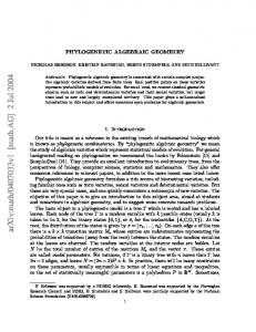
Figure 1: Typical view of a bounded grand orbit of order n = 2 (thus the loop is of length 2) for f (x) which is a quadratic polynomial (thus two arrows enter every vertex). (a) Example of generic case: f (x) = x2 − 3, shown together with its embedding into the complex-x plane. (b) The same example, f (x) = x2 − 3, only internal tree structure is shown. (c) Example of degenerate case: f (x) = x2 − 1 (only one arrow enters −1, its second preimage is infinitesimally close to 0).
Figure 2: A non-degenerate bounded grand orbit of order n = 5 for cubic f (x). Only internal structure is shown, without embedding into X.
9
and � Fn,k (x; f ) = f ◦(n+k) (x) − f ◦k (x) = Fn+k (x; f ) − Fk (x; f ) = Fn x; f ◦k .
(8)
All periodic orbits Om (f ) ⊂ Sn (f ) whenever m is a divisor of n (in particular, when m = n). Similarly, Om,k (f ) ⊂ Sn,k (f ). This property allows to substitute the study of (bounded) periodic (grand) orbits by the study of roots of maps Fn,k (x; f ). Reshufflings (mergings and decompositions) of (grand) orbits occur when the roots coincide, i.e. when the map becomes degenerate. This property allows to substitute the study of the phase space X (where the orbits and roots are living) by the study of the space M of functions, where the varieties of degenerate functions are known as discriminants D. • On (f ) ⊂ X is a set of zeroes of function Gn (x; f ), which is an irreducible-over-any-field divisor of reducible function Fn (x; f ), Y Gm (x; f ), (9) Fn (x; f ) = m|n
where the product is over all divisors m of n, including m = 1 and m = n. The functions Gn are more adequate for our purposes than Fn , but the Fn are much easier to define and deal with in sample calculations. • Stable periodic orbit of order n is defined by conditions � |(f ◦n )′ (x)| < 1 i.e. |Fn′ (x) + 1| < 1 Gn (x) = 0
(10)
for all its points. This definition is self-consistent because (f ◦n )′ (x) =
n−1 Y
f ′ (f ◦k (x)) =
k=0
Y
f ′ (z),
(11)
z∈orbit
i.e. the l.h.s. is actually independent of the choice of x ∈ On (f ). Other periodic orbits are called unstable. Bounded grand orbits are called stable and unstable when periodic orbits at their ends are stable and unstable respectively. • The set of stable periodic orbits O+ (f ) and its complement: the state of unstable periodic orbits O− (f ). By definition O+ (f ) ∪ O− (f ) = O(f ). • Julia set J(f ) ∈ X is attraction domain of stable periodic orbits of f , i.e. the set of points x ∈ X with orbits O(x; f ), approaching the set of stable orbits: ∀ε > 0 ∃k and ∃zk ∈ O+ (f ): |f ◦k (x) − zk | < ε. This definition refers to non-algebraic structures like continuity. However, the boundary ∂J(f ) is an almost algebraic object, since it actually consists of all the unstable periodic orbits and their grand orbits, which are dense in ∂J(f ): ∂J(f ) = O− (f ) = GO − (f )
(12)
Moreover, each grand orbit ”originates in the vicinity” of O− (f ): generically, every branch of the grand-orbit tree is associated with – ”originates at” – a particular orbit from O− (f ), and when O+ (f ) = ∅ this is a oneto-one correspondence. If O+ (f ) 6= ∅, the ”future” of the grand orbit can be three-fold: it can terminate in a periodic orbit, stable or unstable, approach (tend to) some stable orbit or go to infinity (which can actually be considered as a ”reservoir” of additional stable orbits). If O+ (f ) = ∅, the situation is different: strange attractors can also occur. Description of ∂J(f ) in terms of orbits works even when O+ (f ) = ∅, but then it is not a boundary of anything, the Julia set J(f ) itself is not defined. For a better description of Julia sets see summary in s.3 and s.5.5 below.
10
2.2
Objects, associated with the space M
• The moduli space M of all maps. In principle it can be as big as the set of formal series (6), i.e. can be considered as the space of the coefficients {ak }. Some pieces of theory, however, require additional structures, accordingly one can restrict M to sets of continuous, smooth, locally analytic or any other convenient sets of maps. We assume that the maps are single-valued, and their functional inverses can be described in terms of trees, perhaps, of infinite valence. The safest (but clearly over-restricted) choice is a subspace P ⊂ M of all polynomials with complex coefficients, which, in turn, can be decomposed into spaces of polynomials of particular degrees d: P = ∪∞ c) ⊂ M, with ak (~c) d Pd . One can also consider much smaller subspaces: families µ(~ in (6) parameterized by several complex parameters ~c = (c1 , c2 , . . .). Most examples in the literature deal with one-parametric families. • The moduli subspace M◦n ⊂ M of shifted n-iterated maps, consisting of all maps F : X −→ X which have the form (7) for some f (x). The shift by x is important. Eq.(7) defines canonical mappings Iˆn : M −→ M◦n , which can be also written in terms of the coefficients: for f (x) parameterized as in eq.(6), and Fn (x; f ) = f ◦n (x) − x =
∞ X
(n)
ak xk
k=0
we can define Iˆn as an algebraic map (n) Iˆn : {ak } −→ {ak }
(13)
(n) where all ak are polynomials of {al }.6 Inverse map Iˆn−1 is defined on M◦n only, not on entire M, but is not single-valued. In what follows we denote the pull-back of Iˆn by double star, thus (Iˆn f )∗∗ = f (while Iˆn−1 (Iˆn f ) can contain a set of other functions in addition to f , all mapped into one and the same point Iˆn f of M◦n ). The map Iˆn can be restricted to polynomials of given degree, then
Iˆn : Pd −→ Pdn
(14)
embeds the (d + 1)C -dimensional space into the (dn + 1)C one as an algebraic variety.7 Like in (14), often ∗∗ µ◦n = Iˆn (µ) 6⊂ µ. One can, however, use a pull-back to cure this situation: [B ∩ µ◦n ] ⊂ µ for any B ⊂ M. In the studies of grand orbits more general moduli subspaces are involved: M◦(n,k) ⊂ M, consisting of all maps of the form (8) for some f . • Similarly, the functions Gn (x; f ) define another canonical set of mappings, Jˆn : M −→ Mn . into subspaces Mn ⊂ M, consisting of all functions which have the form Gn (x; f ) for some f . These are, however, somewhat less explicit varieties than M◦n , because such are the functions Gn (x; f ) – defined as irreducible constituents of Fn (x; f ). Still, they are quite explicit, say, when f are polynomials of definite degree, and they are more adequate to describe the structures, relevant for discrete dynamics. The J-pullback will be denoted by a single star. (0)
(1)
6 In order to avoid confusion we state explicitly that a = 0 and ak = ak − δk,1 . Also M◦1 = M, but in general analogous k relation is not true for subsets µ ⊂ M: µ◦1 does not obligatory coincide with µ, it differs from it by a shift by x. 7 For example, (P ) 2 ◦2 is embedded into P4 as algebraic variety:
8A2 (D + 1) − 4ABC + B 3 = 0,
This follows from
64A2 (4AB 2 E + B 3 − 4A2 (D + 1)2 )3 = B 3 (16A2 (D + 1) − B 3 )3 3 4
Ax4 + Bx3 + Cx2 + Dx + E = (ax2 + bx + c)◦2 − x =
= a x + 2a2 bx3 + (ab2 + ab + 2a2 c)x2 + (2abc + b2 − 1)x + (ac2 + bc + c).
Note, that because of the shift by x one should be careful with projectivization of this variety.
11
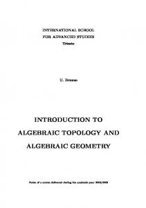
Figure 3:
Schematic view of inter-relations between the subsets M◦n , µ◦n and D◦n .
• Discriminant variety D ⊂ M consists of all degenerate maps f , i.e. such that f (x) and its derivative f ′ (x) have a common zero. It is defined by the equation D(f ) = 0 in M, where D(f ) is the square of the Van-der-Monde product of roots differences: Y Y for f (x) ∼ (x − rk )D(f ) ∼ (rk − rl ). k
k6=l
Restrictions of discriminant onto the spaces of polynomials of given degree, D(Pd ) = D ∩ Pd , are algebraic varieties in Pd , because D(f ) is a polynomial (of degree 2d − 1) of the coefficients {ak } in representation (6) of f (while roots themselves are not polynomial in {ak } the square of Van-der-Monde product is, basically, by Vieta’s theorem). Discriminant variety D has singularities of various codimensions k in D, associated with mergings of k + 2 roots of f . • Resultant variety R ⊂ M× M consists of pairs of maps f (x), g(x) which have common zero. It is defined by the equation R(f, g) = 0, and for f (x) ∼
Y k
(x − rk ) and g(x) ∼
Y (x − sl ) l
Y R(f, g) ∼ (rk − sl ). k,l
Again, if f and g are polynomials, resultant is a polynomial in coefficients of f and g. Resultant variety has singularities when more that one pair of roots coincide. Discriminant can be considered as appropriate resultants’ derivative at diagonal f = g. Higher resultants varieties in M × . . . × M are also important for our purposes, but will not be considered in the present paper. • Intersections of D and R with subspaces like M◦n and Mn , i.e. D◦n = D ∩ M◦n , R◦(m,n) = R ∩ (M◦m × ˆ M◦n ); Dn = D ∩ Mn , Rm,n = R ∩ (Mm × Mm ) consist of disconnected components (see Fig.3). I-pullbacks ∗∗ ∗∗ ˆ D◦n , R◦(m,n) ⊂ M and J-pullbacks Dn∗ = {f : D(Gn (f )) = 0} ⊂ M,
R∗m,n = {f : R(Gm (f ), Gn (f )) = 0} ⊂ M also consist of numerous components, disjoint and touching. Particular families µ ⊂ M intersect these singular varieties and provide particular sections ∂M (µ) of this generic structure: the universal discriminant (or resultant) variety ∞ ∞ ∞ [ [ [ R∗m,n Dn∗ D∗ = R∗ = Rn = n,m=1
n=1
12
n=1
which is the boundary of the Universal Mandelbrot set ∂M (M). • For a given family of maps µ ⊂ M the boundary of algebraic Mandelbrot set ∂M (µ) ⊂ µ is defined ˆ as a J-pullback ∗ ∗ ∞ ∂M (µ) = ∪∞ n=1 (Dn ∩ µ) = (D ∩ (∪n=1 µn )) =
= µ ∪ (∪∞ n=1 {f : D(Gn (f )) = 0})
(15)
• Varieties D∗∗ , R∗∗ , D∗ , R∗ – and thus the boundary of algebraic Mandelbrot space ∂M – can be instead considered as pure topological objects in M independent of any additional algebraic structures, needed to define Fn , Gn , discriminant and resultant varieties D and R. For example, D1∗∗ = D1∗ consists of all maps f ∈ M with two coincident fixed points. Higher components Dn∗ ⊂ Dn∗∗ consist of maps f , with two coincident fixed points of their n-th iteration (for Dn∗∗ ) and such that any lower iteration does not have coincident points (for Dn∗ ). Resultants consist of maps f with coinciding fixed points of their different iterations. Fixed points and iterated maps are pure categorial notions, while to define coincident points one can make use of topological structure: two different fixed points merge under continuous deformation of f in M. • Stability domain of the periodic order-n orbits Sn ⊂ M is defined by the system (10): if a root x of Gn (f ) is substituted in to inequality, it becomes a restriction on the shape of f , i.e. defines a domain in M. This domain is highly singular and disconnected. For a family µ ⊂ M we get a section Sn (µ) = Sn ∩ µ, also singular and disconnected. • Mandelbrot set M (M) ⊂ M is a union of all stability domains with different n: M = ∪∞ n=1 Sn ,
M (µ) = ∪∞ n=1 Sn (µ) = M ∩ µ.
(16)
Definitions (16) and (15) leave obscure most of the structure of Mandelbrot set and its boundary. Moreover, even consistency of these two definitions is not obvious.8 For better description of Mandelbrot set see s.3 below. • Above definitions, at least the algebraic part of the story, can be straightforwardly extended from orbits to grand orbits and from maps Fn (f ) and Gn (f ) to Fn,k (f ) and Gn,k (f ). The maps Gn,k (x; f ), which define k-th pre-orbits of periodic order-n orbits are not obligatory irreducible constituents of Fn,k (x; f ) (what is the case for k = 0). They are instead related to peculiar map z: M→X associating with every f ∈ M the points x ∈ X with degenerate pre-image: zf = {z : D(f (x) − z) = 0}. Generalizations of Mandelbrot sets to k ≥ 1 are called secondary Mandelbrot sets. The Grand Mandelbrot set is the union of secondary sets with all k ≥ 0. Bifurcations of Julia sets with the variation of f inside µ ⊂ M are captured by the structure of Grand Mandelbrot set. We see that, the future theory of dynamical systems should include the study of two purely algebro-geometric objects: (i) the universal discriminant and resultant varieties D ⊂ M and R ⊂ M × M, ∗ ∗ (ii) the map µ −→ µ ˇ = ∪∞ n=1 µn and the pull-backs D ⊂ M and R ⊂ M. It should investigate intersections of D and µ ˇ and R with µ ˇ×µ ˇ and consider further generalizations: to multi-dimensional phase spaces X and to continuous iteration numbers n. It is also interesting to understand how far one can move with description of R∗ and universal Mandelbrot space by pure topological methods, without the ring and other auxiliary algebraic structures. 8 It deserves emphasizing that from algebraic perspective there is an essential difference between the Mandelbrot and Julia sets themselves and their boundaries. Boundaries are pure algebraic (or, alternatively, pure topological) objects, while entire spaces depend on stability criteria, which, for example, break complex analyticity and other nice properties present in the description of the boundaries.
13
Figure 4:
Divisors tree t[24]. It contains divisor trees for all its divisors: t[12], t[6], t[4], t[3], t[2], t[1], some in several copies.
Figure 5:
2.3
A piece of the forest of multipliers trees. Trails are shown by ”steps”.
Combinatorial objects
• Divisors tree t[n] is a finite rooted tree. Number n stands at the root, and it is connected to all τ (n) − 1 of its divisors k|n (including k = 1, but excluding k = n). Each vertex k is further connected to all τ (k) − 1 of its divisors and so on. The links are labeled by ratios m = n/k ≥ 2 and mi = ki /ki+1 ≥ 2. Number n is equal to product of m’s along every branch. See examples in Fig.4. The number τ (n) of divisors of n = pa1 1 . . . pakk is equal to τ (n) = (a1 + 1) . . . (ak + 1). A generating function (Dirchlet function) has asymptotic X √ (17) D(x) = τ (n) ∼ x log x + (2C − 1) + O( x), n≤x
C – Euler constant. • Multipliers tree Tn is a rooted tree of infinite valence. At the root stands the number n. The branches at every level p are labeled by positive integers mp = 1, 2, 3, 4, . . .. Every vertex at p-th level is connected to the root by a path m1 , m2 , . . . , mp and the product nm1 m2 . . . mp stands in it. The basic forest T = ∪n=1 Tn . A number of times B(n) the number n occurs in the forest T is equal to the number of branches in its divisors tree.
14
Figure 6: A fragment of the basic graph. Only the generating arrows, associated with primes, are shown (to avoid overloading the picture). All compositions of arrows should be added as separate arrows (for example, arrows connect 1 to 4, 6, 8, 9 and all other integers).
The numbers τp (n) of ways to represent n as a product of p integers, i.e. the numbers of times n appears at the p − th level of multipliers tree, are described by the generating function Dp (x) =
X
τp (n) =
n≤x
ζ(s) =
P∞
m=1
1 2πi
Z
c+i∞
c−i∞
ds s p x ζ (s), s
m−s is Riemann’s zeta-function. Note that (17) describes τ (n) = τ2 (n).
• Basic graph B is obtained from the multipliers tree T1 by identification of all vertices with the same numbers, so that the vertices of B are in one-to-one correspondence with all natural numbers. Since T1 was a rooted tree, the graph B is directed: all links are arrows. There are τ (n) − 1 arrows entering the vertex n and infinitely many arrows which exit it and lead to points mn with all natural m.
2.4
Relations between the notions
Relations are summarized in the following table.
15
objects in X
objects in M
map f ↓ iterated maps Fn (f ) ↓ Q Fn (f ) = k|n Gk (f ) ↓ n − periodic f − orbits = = roots of Gn (f ) ↓ coincident roots of Gn (f ) = reshuffling of orbits
moduli space M ∪ spaces M◦n spaces Mk
= =
{D{Gn (f )} = 0} discriminant varieties = = ∂(Mandelbrot set M )
maps Fn,k (f )
spaces M◦(n,k)
ւ
ց
bounded grand f − orbits
unstable periodic orbits = ?
= ∂(Julia set J(f )) =
= roots of Fn,k (f )
?
∂(algebraic Julia set JA (f )) ↓
=
reshuffling of JA (f )
=
?
infinite preimage of BGO ↓ coincident roots of Fn,k (f ) resuffling of BGO =
16
=
{D{Fn,k (f )} = 0}
∂(grand Mandelbrot set)
3
Summary
In this section we briefly summarize our main claims, concerning the structure of Mandelbrot and Julia sets. They are naturally splited in three topics.
3.1
Orbits and grand orbits
This part of the story includes: – The theory of orbit and pre-orbit functions Gn (x; f ) and Gn,k (x; f ). – Classification of orbits, pre-orbits and grand orbits. – Intersections (bifurcations) of orbits and degenerations of grand orbits. – Discriminant and resultant analysis, reduced discriminants dn and resultants rm,n intersections of resultant and discriminant varieties. All these subjects – to different level of depth – are considered in s.4 below and illustrated by examples in ss.5 and 6. Systematic theory is still lacking.
3.2
Mandelbrot sets
Figs.7,a-b show three hierarchical levels of Mandelbrot set: the structure of individual component (M1 in Fig.7,a); existence of infinitely many other components (like M3,α in Fig.7,b), which look practically the same after appropriate rescaling; trails connecting different components Mkα with M1 , which are densely populated by other Mmβ (well seen in the same Fig.7,b). These structures (except for the self-similarity property) are universal: they reflect the structure of the universal Mandelbrot set, of which the boundary is the universal resultant variety R∗ . This means that they do not depend on particular choice of the family µ (above figures are drawn for fc = x4 + c, which is in no way distinguished, as is obvious from similar pictures for some other families, presented in ss.5 and 6). The only characteristics which depend on the family are the sets of indices α, labeling degeneracies: different domains with the same place in algebraic structures. Algebraic structure reflects intersection properties of different subvarieties R∗m,n , while α’s parameterize the intersection subvarieties. To classify the α-parameters one should introduce and study higher resultants and multiparametric families µ ⊂ M, what is straightforward, but (except for introductory examples) is left beyond the scope of the present paper. The main property of the resultant varieties R∗m,n , responsible for the structure of Mandelbrot set, is that they are non-trivial in real codimension two only if n is divisible by m or vice versa. All the rest follows from above-described relation between the resultant varieties and the boundary of Mandelbrot set. Stability domains Sn and Mandelbrot sets M are made out of the same disk-like9 building blocks, but connect these blocks in two different ways. Mandelbrot set and its ”forest with trails” structure reflect the universal (µ-independent) labeling (ordering) of these elementary domains (denoted by σ below), while their sizes, locations are self-similarity properties (which depend on the choice of µ) are dictated by stability equations. 3.2.1
Forest structure
For any family of maps µ Mandelbrot set M (µ) has the following hierarchical structure, see Fig.7,a (for particular µ some components – or, better to say, their intersections with µ – can be empty): M (µ) consists of infinitely many disconnected components (of which only one is clearly seen in Fig.7,a and some others are revealed by zooming in Fig.7,b), [ M (µ) = Mkα (µ), Mkα ∩ Mlβ = ∅, if k 6= l or α 6= β, k,α
labeled by natural number k and an extra index α, belonging to the µ-dependent set νk (µ). For polynomial f the set is finite, its size will be denoted by |νk (µ)|. Every component Mkα (µ) is a union of elementary domains, each with topology of a disc (interior of a (2D − 1)R -dimensional sphere if µ is a DC -parametric family), which form a tree-like structure. Vertices of the tree Tkα – the skeleton of Mkα – are associated with ”centers” of elementary domains, a link connects two 9 In the case of multi-parametric families µ ⊂ M, when dimension of components of Mandelbrot set M (µ) is equal to dim µ , ”disc” may be not a very adequate name. In fact, these components look more like interiors of cylinders and tori rather than balls.
17
Figure 7: a) General view of the Mandelbrot set for the family fc (x) = x4 + c. Actually, only the M1 component is well seen. Arrow points at another component, M3,α , shown unlarged in b). The structure of the trail between M1 and M3,α (almost unobservable in this picture) is also seen in b). Z3 -symmetry of the picture is due to invariance of equations like x4 + c = x under the transformation x → e2πi/3 x, c → e2πi/3 c. Associated Julia set has Z4 symmetry, see Fig.8. b) Enlarged component M3,α , included in the box in a). It looks like exact copy of M1 in a). In fact similarity is approximate, but the deviations are damped by the ratio of sizes, r3 /r1 ≪ 1. In this unlarged picture also the trail is seen between M1 and M3,α and other Mkα component in it.
vertices whenever the two corresponding domains have a common point – and there can be at most one such point, where the two domains actually touch each other. The skeleton is a rooted tree, moreover, it is actually a covering of the multipliers tree Tk , introduced in s.2.3. The difference is that every branch at the level p (p) (p) carrying the label mp has multiplicity |νmp (µ)| and thus an extra label αp ∈ νmp (µ). The union of skeleton trees is the skeleton of the Mandelbrot set – the Mandelbrot forest [ T (M ) = Tkα . k,α
Thus Mkα =
∞ [
(p)
Mkα
p=0 (p) Mkα
∞ [
=
σ
(p)
m1 ,...,mp =1 α1 ,...,αp
�
m1 α1
and, finally, M (µ) = M ∩ µ, ∞ [[ M= k,α p=0
∞ [
σ (p)
m1 ,...,mp =1 α1 ,...,αp
�
m1 α1
� . . . mp kα . . . αp � . . . mp kα . . . . αp
� m1 . . . mp The elementary domains are σ kα and two of them touch at exactly one point, whenever α1 . . . αp they are connected by a link in the powerful tree Tkα , i.e. when p′ = p + 1, and m′i = mi , α′i = αi for all i = 1, . . . , p. (p)
3.2.2
�
Relation to resultants and discriminants
The touching point (map f ∈ µ) belongs to the resultant variety R∗n,n′ , i.e. is a root of R(Gn (f ), Gn′ (f )) = 0, with n = km1 . . . mp and n′ = km1 . . . mp m′p+1 = nm′p+1 . The boundaries of all elementary domains σ (p) with p > 0 are smooth (unless µ crosses a singularity of R), while ∂σ (0) [kα] has a cusp, located at discriminant variety Dk∗ , i.e. at f ∈ µ, satisfying D(Gk (f )) = 0 (σ (0) [kα] itself has a peculiar cardioid form). It is clear that the bigger the family µ, the more intersections it has with the resultant and discriminant varieties, thus the 18
bigger are the sizes of the sets ν (p) (µ). For entire M the indices αp get continuous and parameterize the entire pullbacks of the resultant and discriminant varieties. Every elementary domain σ (p) touches a single domain of the lower level p − 1 and infinitely many domains (p+1) of the next level p + 1 (which are labeled by all integer m = mp+1 ≥ 2 and α = αp+1 ∈ νm (µ)). The touching points – belonging to zeroes of R(Gn , Gnm ) with all possible m = mp+1 are actually dense in the boundary ∂σ (p) , i.e. the boundary can be considered as a closure of the sets of zeroes. 3.2.3
Relation to stability domains � � m1 . . . mp (p) As already mentioned, every σ kα is characterized by an integer n = km1 . . . mp . Someα1 . . . αp (p)
time, when other parameters are inessential, we even denote it by σn . Stability domain Sn (µ), defined by the conditions (10) is a union of all σ(µ) with the same n. This implies, that Sn is actually a sum over all branches of divisor tree t[n], introduced in s.2.3. Then p is the length of the branch at k is its end-link. Other links carry numbers m1 , . . . , mp . The only new ingredient is addition of extra parameters α at every step. This means that we actually need α-decorated divisor trees (for every family µ), which we denote t˜[n](µ) and imply that links (p) at p-th level carry pairs mp , αp with αp ∈ νmp (µ), and sum over decorated trees imply summation over α’s. In other words, the elementary domains σ are actually labeled by branches of the decorated trees, B t˜, and [ Sn = σn [B t˜] = B t˜[n]
=
∞ [
p=0
[ m k|n
α∈νk
[
σ (p)
1 ,...,mp : n=km1 ...mp (p) (1) α1 ∈νm1 ,...,αp ∈νmp
�
m1 α1
� . . . mp kα . . . αp
(18)
It remains an interesting problem to prove directly that eqs.(10) imply decomposition (18). 3.2.4
Critical points and locations of elementary domains
Let wf denote critical points of the map f (x): f ′ (wf ) = 0. Then (f ◦n )′ (wf ) = 0, i.e. the critical points always belong to some stable orbit, see (10). This orbit is periodic of order n provided Gn (wf ; f ) = 0.
(19)
This is an equation on the map f and its solutions define points f in the lie inside which � family µ ⊂ M, � m1 . . . mp (p) stability domain Sn , and, actually, inside certain elementary domains σ kα . In fact this α1 . . . αp is a one-to-one correspondence: solutions to eq.(19) enumerate all the elementary domains. This implies the following pure algebraic description of the powerful forest of M (µ) (formed by the coverings Tkα of the multipliers trees Tk ). All vertices of the graph are labeled by solutions of (19) and accordingly carry indices n. Links are labeled by roots of the resultants R(Gm (f ), Gn (f )), with appropriate m and n (standing at the ends of the link). α-parameters serve to enumerate different solutions of (19) and different roots of the same resultants. Critical points wf also play a special role in the study of bifurcations of grand orbits and Julia sets, see s.4.6. 3.2.5
Perturbation theory and approximate self-similarity of Mandelbrot set
For concrete families µ ⊂ M a kind of approximated perturbation theory can be developed in the vicinity of solutions f = f0 to (19). Namely, one can expand equations (10), which define the shape of stability domain (and thus of the elementary domains σ[kα]), in the small vicinity of the point (x, f ) = (wf0 , f0 ) and, assuming 19
that the deviation is small, substitute original exact equations by their approximation for small deviations. Approximate equations have a universal form, depending only on the symmetry of the problem. This explains why in many examples (where this method is accurate enough) all the components Mkα of Mandelbrot set look approximately the same, i.e. why the Mandelbrot set is approximately self-similar (see Fig.7,b) and help to classify the components of stability domain. The same method can be used to investigate the shape (not just structure) of Julia sets. See in sec.4.9.4 below an example of application of this procedure to the map families fc = xd + c. 3.2.6
Trails in the forest
The last level of hierarchy in the structure of Mandelbrot set is represented by trails, see Fig.7,b. Despite the components Mkα do not intersect (do not have common points), they are linked by a tree-like system of trails: each Mkα is connected to M1 by a single trail τkα , which is densely populated by some other components Mlβ . The trail structure is exhaustively described by triangle embedding matrix, τ = {τ [kα, lβ]} with unit entry when one trail is inside another, τlβ ⊂ τkα , and zero entry otherwise. If locations of all Mkα in parameter-~c space are known (for example, evaluated with the help of the perturbation theory from s.3.2.5), then embedding matrix fully describes the trails. It is unclear whether any equations in parameter space µ can be written, which define the shape of trails. Embedding matrix seems to be universal, i.e. does not depend on the choice of the family µ. If true, this means that the trail structure is indeed a pertinent characteristic of Mandelbrot/resultant variety, not of its section by µ. However, as usual, the universal structure is partly hidden because of the presence of non-universal degeneracies, labeled by α-parameters (at our level of consideration, ignoring higher resultants): concrete trail systems τ (µ) are coverings of presumably-universal system. Trail structure requires further investigation and does not get much attention in the present paper.
3.3
Sheaf of Julia sets over moduli space
The structure of Julia set J(f ) is also hierarchical and it depends on the position of the map f in Mandelbrot set, especially on its location in Mandelbrot i.e. on the set of parameters {kα, p, mi αi }, labeling the forest, � � m . . . m 1 p elementary domain σ (p) kα which contains f . Since in this paper we do not classify αα1 . . . αp dependencies, only the numbers k (labeling connected component), p (labeling the level) and m1 , . . . , mp will be interpreted in terms of J(f ) structure. Julia set is a continuous deformation of a set of discs (balls), which – the set – depends on k; increase of p by every unit causes gluing of infinitely many points at the boundary, at every point exactly mp points are glued together. Every elementary domain is associated with a set of stable orbits (often there is just one), contained inside the Julia set together with their grand orbits. All other (i.e. unstable) periodic orbits and their grand orbits belong to the boundary of Julia set and almost each particular grand orbit fills this boundary densely. At the touching point between two adjacent elementary domains the stable orbit approaches the boundary ∂J from inside J (perhaps, it is better to say that the boundary deforms and some of its points – by groups – approach the orbit which lies inside J), intersect some unstable orbit and ”exchange stability” with it. Their grand orbits also intersect. The ratio of orders of these two orbits is mp and every mp points of unstable grand orbit merge with every point of the stable one, thus strapping the disc at infinitely many places (at all points of the merging grand orbits) and pushing its sectors into bubble-like shoots, see Fig.8. As f transfers to the elementary domain at level p + 1, the new stable orbit (the one of bigger order) quits the boundary and immerses into Julia set, while the orbit of smaller order, which is now unstable, remains at its boundary: the singularities, created when the grand orbits crossed, can not disappear. One can say that every link of the forest describes a phase transition of Julia set between neighboring elementary domains. An order parameter of this transition is the distance between approaching stable and unstable orbits on one side, looking as the contact length between emerging components of Julia set, and the angle between these components on the other side, when they are already separated except for a single common point. Both quantities vanish at transition point (i.e. when f is at the touching point between two domains in the Mandelbrot set). If we move around the transition point in M, there is a non-trivial monodromy (the Julia set gets twisted), but on the way one should obligatory pass through the complement of Mandelbrot set,
20
where the discs – which form Julia set – disappear, only the boundary remains, Julia set has no ”body”, only boundary, and exact definition of monodromy is hard to give. Julia sets can change structure not only when stable orbit intersects with unstable one – what happens when the corresponding elementary domains σ of Mandelbrot set touch each other, – but also when unstable grand orbits at the boundary ∂J(f ) cross or degenerate. Such events are not reflected in the Mandelbrot set itself: a bigger Grand Mandelbrot set, which contains all zeroes of D(Fn,k ) and R(Fn,k , Fm,l ) on its boundary, should be introduced to capture all the bifurcations of Julia set. See s.5.5 for some more details about Julia sets and their bifurcations.
21
(0)
Figure 8: The typical forms of the Julia set for the map fc = x4 + c and c ∈ M1 . a) c in the center of σ1 (c = 0). Z4 symmetry of the picture is due to the symmetry of the map fc . Associated Mandelbrot set has symmetry Z3 , see Fig.7,a. b) c at the touching √ (0) (1) 5 1/3 point σ1 ∪ σ2 (c = 16 2 (1 + i 3)). Infinitely many pairs of points on the unit circle (a) are identified to provide this pattern. √ (0) (1) c) c at another touching point σ1 ∪ σ3 (c = 81 (9 + i 111 3)1/3 ). Infinitely many triples of points on the unit circle (a) are (1)
identified to provide this pattern. d) c inside σ2 (c = 0.45 + i 0.8). This is a further deformation of (a) in the direction of (b). Once appeared in (b) the merging points at the boundary and straps of the disc caused by this merging of boundary points do not disappear, but angles between the external bubbles increase from the zero value which they have in (b). They will turn into 2π/2 (1) (1) (2) (1) (2) and bridges become needles when c reaches the boundary of σ2 , say an intersection point σ2 ∪ σ4 (e) or σ2 ∪ σ6 (f). e) c at (1)
(2)
(1)
(2)
the touching point σ2 ∪ σ4 (c ≈ 0.56 + 0.97i). f) c at the touching point σ2 ∪ σ6 (c ≈ 0.309 − 0.862i). A mixture of merging pairs and triples is clearly seen. The bridges for pairs became needles, while triplets are touching. Angles between triplets will (2) increase as c goes inside σ6 and reach 2π/3 at its boundary, and so on. Arrows point the positions of Julia sets shown in Fig.8 in the Mandelbrot set. The ”Julia sheaf” is obtained by ”hanging” the corresponding Julia set over each point of the Mandelbrot set. At the boundary of Mandelbrot set the Julia sets are reshuffled and the task of the theory is to describe this entire variety (the sheaf) and all its properties, both for the universal Mandelbrot set and multi-dimensional Julia sets associated with multicomponent maps, and for the particular sections, like the one-parametric family of single-component quartic maps, f (x; c) = x4 + c shown in this particular picture.
22
4 4.1
Fragments of theory Orbits and reduction theory of iterated maps
In discrete dynamics trajectories are substituted by orbits and closed trajectories – by periodic orbits On of the finite order n. Different orbits have no common points, and f acts on each On by cyclic permutation of points. All points of every On belong to the set Sn (f ) of roots of the function Fn (x; f ) = f ◦n (x) − x. The map f generates the action of cyclic group fˆ(n) on Sn (f ), and this set is decomposed into orbits of fˆ(n) of the orders k, which are divisors of n (all On with k = n are among them). If n is divisible by k, then Fn (x) is divisible by Fk (x), and in general Fn decomposes into irreducible constituents: τ (n)
Fn (x; f ) =
Y
Gk (x; f )
(20)
k|n
with a product over all possible τ (n) divisors k of n (including k = 1 and k = n). The number of periodic orbits of order n is equal to Nn (f )/n, where Nn (f ) is the number of roots of Gn (x; f ). Irreducibility means that Gk are not decomposable into simpler constituents in an X- and f -independent way (of course, when Gk (x) are polynomials they can be decomposed into products of monomials over C, but this decomposition will not take place over R). Among the tasks of the theory is the study of reducibility of the sets Sn (f ), the ways they decompose into orbits and the ways this decomposition changes under the deformations of f within µ ⊂ M. Since the story is essentially about the roots of functions, it gets much more transparent in the complex setting than in the real one. Also, the entire theory is naturally a generalization from the case of the polynomial functions f ∈ P ⊂ M. Obviously, for f ∈ Pd ⊂ P, Fn ∈ Pdn , and Gk (x) in (20) is a polynomial of certain degree Nk (d). If d = p is prime, then the group fˆ(n) = Zn and is isomorphic to the Galois group over Fp of the cyclotomic polynomial n xp − x (while the Galois group of f itself over C is trivial). If instead n = p is prime, then d out of the dp roots of Fp (x) are also the roots of F1 (x), i.e. are invariant points (orbits of order one) of f , while the remaining p dp − d roots decompose into d p−d orbits of order n = p. According to (20) the numbers Nn (d) for f ∈ Pd can be defined recursively: from τ (n) X Nk (d) = deg Fn = dn k|n
it follows, that Nn (d) = dn −
X
Nk (d).
k|n
k t0 . If a new root xi (t′′ ) belongs to an f -orbit O, then all the elements of O belong to the f -invariant domain C − R for t′ < t0 and ”simultaneously come” to the f -invariant ¯ come to the real axis R simultaneously, one can domain R at t = t0 . Since elements of O and its conjugate O say, that real roots ”are born in pairs” at t = t0 .
4.3
Discriminants and resultants for iterated maps
General comments on the definitions of discriminants and resultants (including the non-polynomials case) are collected in s.4.11 below. However, for iterated maps these quantities are highly reducible. Discriminant variety is defined by the equation D(f ) = 0 where, for polynomial f , D(f ) is of the coefficients {a}, see eq.(51) below. Similarly,�D(Fn ) is � the polynomial a polynomial of the coefficients a(n) (a) and the resultant R(Fn , Fm ) is a polynomial of coefficients a(n) (a) � and a(m) (a) . Since function Fn (x) is reducible over any field (e.g. over R as well as over C), see (20), the resultant factorization rule (54) implies: Y Y D(Gk ) R2 (Gk , Gl ). (21) D(Fn ) = k|n
k,l|n
k>l
However, this is only the beginning of the story. Despite Gk (x) are irreducible constituents of Fn (x), the resultants R(Gk , Gk/m ) and discriminants D(Gk ) are still reducible: R(Gk , Gl ) = rl (Gk , Gl ), l < k, n Y Y rk−l (Gk , Gl ), D(Gk ) = dk (Gk ) Rm−1 (Gk , Gk/m ) = dk (Gk ) m>1
l|k
thus
D(Fn ) =
Y k|n
dk (Gk )
Y l|k
rk+l (Gk , Gl ) .
(22)
Indeed, whenever a resultant vanishes, a root of some Gk/m coincides with that of Gk and then – since roots of Gk form orbits of order k – the k roots should merge by groups of m into l = k/m roots of Gk/m , and there are exactly l such groups. In other words, whenever a group of m roots of Gk merges with a root of Gk/m , so do l = k/m other groups, and R(Gk , Gk/m ) is an l-th power of an irreducible quantity, named r(Gk , Gk/m ) is (22). In a little more detail, if α1 , . . . , αk with k = lm are roots of Gk and β1 , . . . , βl are those of Gk/m , then α1 = β1 implies, say, that α1 = . . . = αm = β1 , αm+1 = . . . = α2m = β2 , ... αm(l−1)+1 = . . . αlm = βl . Then in the vicinity of this point l Y Y (αi − βs ) ∼ R(Gk , Gl ) ∼ i,s
s=1
sm Y
i=(s−1)m+1
(αi − βs )
(factors, which do not vanish, are omitted). Internal products are polynomials of the coefficients of f with first-order zeroes (the roots themselves are not polynomial in these coefficients!), and only external product enters our calculus and provides power l in the first line of eq.(22). 25
Similarly, D(Gk ) ∼
l Y ∼ r,s=1
sm Y
i 1 are the outcome of discriminant/resultant analysis in the sector of G1 and G1,1 , responsible for fixed points and their first pre-images. 4.7.4
Sector (n, s) = (1, s)
For a fixed point x1 = f (x1 ) we denote f ′ = f ′ (x1 ), f ′′ = f ′′ (x1 ). Then for x = x1 + χ we have: ! (n−1) 1 ′′ f ′ 2 ′n + O(χ ) Fn (x) = χ(f − 1) 1 + χf 2 f′ − 1 and
� � 1 ′′ ′ 2 Gk (x) = gk (f ) 1 + χf hk (f ) + O(χ ) , 2 ′
where gk (β) are irreducible circular polynomials (which will appear again in s.6) and hk (β) are more sophisticated (with the single exception of h1 they are also polynomials). The first several polynomials are: g1 (β) = β − 1 g2 (β) = β + 1 g3 (β) = β 2 + β + 1 g4 (β) = β 2 + 1 g5 (β) = β 4 + β 3 + β 2 + β + 1 g6 (β) = β 2 − β + 1
...
h1 g1 (β) = 1 h2 (β) = 1 h3 (β) = β + 1 h4 (β) = β(β + 1) h5 (β) = β 3 + β 2 + β + 1 h6 (β) = β 4 + β 3 + β 2 − 1
Making use of Fn,s = Fn+s − Fs and of decomposition formula (27), it is straightforward to deduce: G1,1 (x) =
1 F2 − F1 = f ′ + χf ′′ (f ′ + 1) + O(χ2 ), G1 2
1 f ′ + 1 − 2 ′′ 1 G1,1 (x) − f ′ (x) = f + O(χ) = f ′′ + O(χ), G1 (x) 2 f′ − 1 2 32
as we already know. Here and below f ′ (x) = f ′ + χf ′′ + O(χ2 ). Further, recursively, G1,s (x) =
Fs+1 − FS 1 s−1 = f ′ + χf ′′ (f ′ + 1)f ′ + O(χ2 ), G1 G1,1 . . . G1,s−1 2 s
s−1
− 2 ′′ 1 f′ + f′ 1 G1,s (x) − f ′ (x) s−1 s−2 = f + O(χ) = f ′′ (f ′ + 2f ′ + . . . + 2) + O(χ), ′ G1 (x) 2 f −1 2
i.e. G1,s (x) = f ′ (x) mod G1 (x) and, as generalization of (30) and (31), we obtain for all s Y r1|1,s = R(G1 , G1,s ) ∼ R(G1 , f ′ ) ∼ G1 (wf ; f ) = w1 . wf
4.7.5
Sector (n, s) = (2, s)
For consideration of the sector (n, s) = (2, s) we need to consider the vicinity of another stable point x2 , which belongs to the orbit of order two, i.e. satisfies f (f (x2 )) = x2 , but x˜2 = f (x2 ) 6= x2 . Denote f ′ = f ′ (x2 ), f˜′ = f ′ (˜ x2 ) = f ′ (f (x2 )), f ′′ = f ′′ (x2 ), f˜′′ = f ′′ (˜ x2 ) = f ′′ (f (x2 )). For x = x2 + χ we have: 1 F1 (x) = G1 (x) = (˜ x2 − x2 ) + χ(f ′ − 1) + χ2 f ′′ + O(χ3 ), 2 � � � 1 � 2 F2 (x) = G1 (x)G2 (x) = χ f ′ f˜′ − 1 + χ2 f ′′ f˜′ + f˜′′ f ′ + O(χ3 ), 2 � � 1 � � 3 F3 (x) = G1 (x)G3 (x) = (˜ x2 − x2 ) + χ f ′2 f˜′ − 1 + χ2 f ′′ f ′ f˜′ + f˜′′ f ′ + f ′′ (f ′ f˜′ )2 + O(χ3 ), 2 ... Then G2,1 (x) =
F2,1 F1 (F3 − F1 ) = = G1 G2 G1,1 (F2 − F1 )F2
(˜ x2 − x2 ) + χ(f ′ − 1) + 12 χ2 f ′′ + O(χ3 ) � � · (˜ x2 − x2 ) − χ(f˜′ − 1)f ′ − 12 χ2 f ′′ (f˜′ − 1) + f˜′′ f ′ 2 + O(χ3 ) � � �� � � 3 χ f ′ f˜′ − 1 f ′ + 12 χ2 f˜′′ f ′ + f ′′ (f ′ f˜′ )2 + f ′ f˜′ − 1 + O(χ3 ) � � � � · = χ f ′ f˜′ − 1 + 12 χ2 f ′′ f˜′ + f˜′′ f ′ 2 + O(χ3 ) !� � 1 χ(f ′ f˜′ − 1) 2 + O(χ ) f ′ + χf ′′ (f ′ f˜′ + 1) + O(χ2 ) , =− 1+ x ˜2 − x2 2 =−
so that ′
′ ˜′
G21 (x) + f (x) = −χ(f f − 1) and
G21 (x) + f ′ (x) =− G2 (x)
is finite at χ = 0. Therefore
�
�
1 ′′ f′ f + 2 x ˜2 − x2
f′ 1 ′′ f + 2 x ˜2 − x2
r2|2,1 = R(G2 , G2,1 ) ∼ −R(G2 , f ′ ) ∼
33
Y wf
�
�
+ O(χ2 )
+ O(χ)
G2 (wf ) = W2 (f ) = w2 (f ).
4.7.6
Summary
In the same way one can consider other quantities, complete the derivation of (29) and deduce the formulas for resultants and discriminants. Like in (33), these decomposition formulas depend explicitly on degree d of the map f (x). In what follows #s = (d − 1)ds−1 denotes the number of s-level pre-images of a point on a periodic orbit, which do not belong to the orbit. Also, wn (f ) enter all formulas multiplied by peculiar d-dependent factors: w ˜n (f )
d=2
w ˜1 = dd w1 , w ˜2 = dd(d−1) w2 , 2 w ˜3 = dd(d −1) w3 , 2 2 w ˜4 = dd (d −1) w4 , 4 w ˜5 = dd(d −1) w5 , 2 3 w ˜6 = dd(d −1)(d +d−1) w6 , ...
d=3
22 = 4, 33 = 27, 22 = 4, 36 = 729, 6 2 = 64, 324 , 12 2 = 4096, 372 230 , 3240 ? 54 2 , 37176 ?
(the last two columns in this table contain the values of numerical factors for d = 2 and d = 3, question marks label the cases which were not verified by explicit MAPLE simulations). Obviously, these factors are made from degree Nd (n) of the map Gn (x), which was considered in s.4.1: w ˜n (f ) = dNd (n) wn (f ). Non-trivial (i.e. not identically unit) resultants are: � w ˜n R(Gm , Gn,s ) = 1 and R(Gk,s , Gn,s′ ) =
�
k#s R(Gk , Gn ) = rk,n #s w ˜n
or, in the form of a table:
34
if m = n, if m 6= n if s′ = s, k < n (actually, k|n) if s < s′
(35)
ns
11
12
13
14
21
22
23
24
31
32
33
34
1 2 3 4 5 ...
w ˜1 1 1 1 1
w ˜1 1 1 1 1
w ˜1 1 1 1 1
w ˜1 1 1 1 1
1 w ˜2 1 1 1
1 w ˜2 1 1 1
1 w ˜2 1 1 1
1 w ˜2 1 1 1
1 1 w ˜3 1 1
1 1 w ˜3 1 1
1 1 w ˜3 1 1
1 1 w ˜3 1 1
-
w ˜1#1 w ˜1#2 w ˜1#2 w ˜1#2 w ˜1#2
w ˜1#1 w ˜1#2 w ˜1#3 w ˜1#3 w ˜1#3
w ˜1#1 w ˜1#2 w ˜1#3 w ˜1#4 w ˜1#4
#1 r12 1 1 1 1 1
1
w ˜1#1 w ˜1#1 w ˜1#1 w ˜1#1 w ˜1#1
1 1
1 1 1
1 #2 r13 1 1 1 1
1 1 #3 r13 1 1 1
1 1 1
1 1
#1 r13 1 1 1 1 1
#4 r13 1 1
21 22 23 24 25 26 ...
#1 r12 1 1 1 1 1
1 #2 r12 1 1 1 1
1 1
1 1 1
31 32 33 34 35 ...
#1 r13 1 1 1 1
41 42 43 44 45 ...
11 12 13 14 15 16 ...
1 #2 r13
#3 r12 1 1 1
1 1
1 1 1
#3 r13 1 1
#1 r14 1 1 1 1
1 #2 r14 1 1 1
1 1
51 52 53 54 55 ...
#1 r15 1 1 1 1
1 #2 r15 1 1 1
61 62 63 64 65 ...
#1 r16 1 1 1 1
1 #2 r16 1 1 1
#3 r14 1 1
1 1 #3 r15 1 1
1 1 #3 r16 1 1
#4 r12 1 1
1 1 1 #4 r13 1
1 1 1 #3 r14 1
1 1 1 #4 r15 1
1 1 1 #4 r16 1
#2 r12
1 1 1 1
#3 r12 1 1 1
w ˜2#1 w ˜2#1 w ˜2#1 w ˜2#1 w ˜2#1
w ˜2#1 w ˜2#2 w ˜2#2 w ˜2#2 w ˜2#2
w ˜2#1 w ˜2#2 w ˜2#3 w ˜2#3 w ˜2#3
w ˜2#1 w ˜2#2 w ˜2#3 w ˜2#4 w ˜2#4
1 1 1 1 1 1
1 1 1 1 1 1
1 1 1 1 1 1
1 1 1 1 1 1
1 1 1 1 1
1 1 1 1 1
1 1 1 1 1
1 1 1 1 1
w ˜3#1 w ˜3#1 w ˜3#1 w ˜3#1
w ˜3#1 w ˜3#2 w ˜3#2 w ˜3#2
w ˜3#1 w ˜3#2 w ˜3#3 w ˜3#3
w ˜3#1 w ˜3#2 w ˜3#3 w ˜3#4
2 )#1 (r24 1 1 1 1
1 2 )#2 (r24 1 1 1
1 1 2 )#3 (r24 1 1
1 1 1 2 )#4 (r24 1
1 1 1 1 1
1 1 1 1 1
1 1 1 1 1
1 1 1 1 1
1 1 1 1 1
1 1 1 1 1
1 1 1 1 1
1 1 1 1 1
1 1 1 1 1
1 1 1 1 1
1 1 1 1 1
1 1 1 1 1
2 )#1 (r26 1 1 1 1
1 2 )#2 (r26 1 1 1
1 1 2 )#3 (r26 1 1
1 1 1 2 )#4 (r26 1
3 )#1 (r36 1 1 1 1
1 3 )#2 (r36 1 1 1
1 1 3 )#3 (r36 1 1
1 1 1 3 )#4 (r36 1
#4 r12
Similarly, for discriminants: #s/#1
D(Gn,s ) ∼ D(Gn )#s w11
35
s Y
r=2
#s/#r Wn,r =
= dnn
Y k|n
k 0 (if such r and r do not exist, i.e. s ≤ n, δ(n, s) = 0). The first few values of δ(n, s) are listed in the table (stars substitute too lengthy expressions):
n\s
1
2
3
4
5
6
7
8
9
10
1 2 3 4 5 6 7 8 9 10 ...
0 0 0 0 0 0 0 0 0 0
1 0 0 0 0 0 0 0 0 0
d+1 1 0 0 0 0 0 0 0 0
d2 + d + 1 d 1 0 0 0 0 0 0 0
d3 + d2 + d + 1 d2 + 1 d 1 0 0 0 0 0 0
* d3 + d d2 d 1 0 0 0 0 0
* d4 + d2 + 1 d3 + 1 d2 d 1 0 0 0 0
* d5 + d3 + d d4 + d d3 d2 d 1 0 0 0
* * d5 + d2 d4 + 1 d3 d2 d 1 0 0
* * d6 + d3 + 1 d5 + d d4 d3 d2 d 1 0
...
The first few discriminants are listed in the table (Dn = D(Gn ), not to be confused with irreducible dn ; the last two columns contain numerical factors for d = 2 and d = 312 ): 12 Numerical
s
factors are equal to dd (sd−s−1)#n (d) , where the sequences #n (d) are 1, 1, 3, 6, 15, . . . for d = 2 and 1, 2, . . . for d = 3. One can observe that #n (d) = degc Gn (x; xd + c), but the reason for this, as well as the very origin of numerical factors, here and in eq.(35), remain obscure.
36
ns
D(Gns )
d=3
1 24
−3 327
216
3135
248
3567
2128
?
1 24
36 354
216
?
248
?
2128
?
1 212
324 ?
248
?
2144
?
2384
?
1 224
? ?
296
?
?
?
?
?
D1d−1 w11 d(d−1) d D1 w11 W12 d2 (d−1) d2 d W D1 w11 W12 13 2 d3 (d−1) d3 d d W D1 w11 W12 W13 14 d4 (d−1) d4 d3 W d2 W d W D1 w11 W12 13 14 15
= =
D2d−1 W21 d(d−1) d W D2 W21 22 2 d2 (d−1) d d W D2 W21 W22 23 d3 (d−1) d3 W d2 W d W D2 W21 22 23 24 d4 (d−1) d4 W d3 W d2 W d W D2 W21 22 23 24 25
= =
D3d−1 W31 d(d−1) d W D3 W31 32 2 d2 (d−1) d d W D3 W31 W32 33 d3 (d−1) d3 W d2 W d W D3 W31 32 33 34 d4 (d−1) d4 W d3 W d2 W d W D3 W31 32 33 34 35
= =
= =
45
D4d−1 W41 d(d−1) d W D4 W41 42 2 d2 (d−1) d d W D4 W41 W42 43 d3 (d−1) d3 W d2 W d W D4 W41 42 43 44 d4 (d−1) d4 W d3 W d2 W d W D4 W41 42 43 44 45
=
4(d−1) 3(d−1) 2(d−1) d4 r14 r24 w41 4d(d−1) 3d(d−1) 2d(d−1) d d4 r14 r24 w41 w42 4d2 (d−1) 3d2 (d−1) 2d2 (d−1) d2 d d4 r14 r24 w41 w42 w43 4d3 (d−1) 3d3 (d−1) 2d3 (d−1) d3 d2 d d4 r14 r24 w41 w42 w43 w44 4d4 (d−1) 3d4 (d−1) 2d4 (d−1) d4 w d3 w d2 w d w d4 r14 r24 w4 w41 42 43 44 45
51 52
D5d−1 W51 d(d−1) d W D5 W51 52
= =
5(d−1) 4(d−1) d5 r15 w51 5d(d−1) 4d(d−1) d d5 r15 w51 w52
1 260
? ?
61 62 ...
D6d−1 W61 d(d−1) d W D6 W61 62
= =
6(d−1) 5(d−1) 4(d−1) 3(d−1) d6 r16 r26 r36 w61 6d(d−1) 5d(d−1) 4d(d−1) 3d(d−1) d d6 r16 r26 r36 w21 w22
1 ?
? ?
11 12 13 14 15 21 22 23 24 25 31 32 33 34 35 41 42 43 44
4.7.7
= = =
= = =
= = =
= =
d1d−1 w11 d(d−1) d w d1 w1 w11 12 d2 (d−1) d+1 d2 d d1 w1 w11 w12 w13 d3 (d−1) d2 +d+1 d3 d2 d d1 w1 w11 w12 w13 w14 4 d (d−1) d3 +d2 +d+1 d4 d3 d2 d w11 w12 w13 w14 w15 d1 w1
d=2
2(d−1) d−1 d2 r12 w21 2d(d−1) d(d−1) d d2 r12 w21 w22 2d2 (d−1) d2 (d−1) d2 w d w d2 r12 w2 w21 22 23 2d3 (d−1) d3 (d−1) d d3 d2 d d2 r12 w2 w21 w22 w23 w24 2d4 (d−1) d4 (d−1) d2 +1 d4 d3 d2 d d2 r12 w2 w21 w22 w23 w24 w25 3(d−1) 2(d−1) d3 r13 w31 3d(d−1) 2d(d−1) d d3 r13 w31 w32 3d2 (d−1) 2d2 (d−1) d2 d d3 r13 w31 w32 w33 3 3d (d−1) 2d3 (d−1) d3 w d2 w d w d3 r13 w3 w31 32 33 34 3d4 (d−1) 2d4 (d−1) d d4 d3 d2 d d3 r13 w3 w31 w32 w33 w34 w35
On interpretation of wn,k
Responsible for degenerations of pre-orbits are intersections with the set {zf } = f ({wf }), which is f -image of the set of critical points of f . Let us describe what happens when {zf } is crossed by pre-orbits of different levels. T • {Gn (f ) = 0} {zf } 6= ∅. Let A be the intersection point, denote its pre-images along the periodic orbit through A−1 , A−2 , . . . , A−n = A, and the pre-images of level s on the pre-image tree through Bi−s (A), where indices i can be further 1 ...i#s ordered according to the tree structure. Points on the level s of the tree, rooted at pre-image A−l will be denoted through Bi−s (A−l ). If A ∈ {zf }, then two of its pre-images coincide. There are two possibilities: 1 ...i#s either these coinciding preimages belong to pre-orbit tree, say B1−1 (A) = B2−1 (A), or one of them lie on the orbit, say B1−1 (A) = A−1 . In the first case wn,1 (f ) = 0, in the second case wn (f ) = 0, and the fact that only two such possibilities exist is reflected in decomposition formula Y Y Gn,1 (wf ) = Wn,1 (f ) = wn (f )wn,1 (f ) Gn (zf ) = zf
wf
(products at the l.h.s. are needed to build up quantities, which depend on the coefficients of f (x), not on their irrational combinations, entering expressions for individual points zf and wf – the latter are roots of f ′ (x)). Let us analyze these two cases in more detail. 37
Figure 9: A periodic orbit of order n and grand-orbit trees, rooted at the points of the orbit. wn (f ) vanishes when (i) a point A on the orbit coincides with an ”irreducible point” from the set {zf }, which is f -image of the set of critical points {wf }, and (ii) when one of the coinciding first pre-images of A is also a point on the orbit. Arrows show the pre-image points of different levels, which coincide when A ∈ {zf } and wn (f ) = 0, i.e. when A−1 = B.
◦ wn (f ) = 0. See Fig.9. Since B1−1 (A) = A−1 exactly one point from {Gn,1 = 0} coincides with exactly one point on {Gn = 0}, thus the resultant has simple zero, R(Gn , Gn,1 ) = rn|n,1 = w ˜n ∼ wn .
Numeric d-dependent factor, distinguishing between w ˜n and wn requires separate explanation. Pre-images of B1−1 (A) – the set of d (different!) points B1−2 (A), . . . , Bd−2 (A) from {Gn,2 = 0} should coincide −1 pairwise with pre-images of A−1 , which are d − 1 points B1−1 (A−1 ), . . . , Bd−1 (A−1 ) from {Gn,1 = 0} and the −2 point A on the orbit, i.e. from {Gn = 0}. Thus the corresponding resultants will have zeroes of orders #1 = d − 1 and one respectively: #1 R(Gn,1 , Gn,2 ) = rn,1|n,2 ∼ wn#1 and −1
R(Gn , Gn,2 ) = rn|n,2 ∼ wn
−3
Next pre-images of A consist of A ∈ {Gn = 0}, #1 = d − 1 points B −1 (A−2 ) ∈ {Gn,1 = 0} and −1 −2 #2 = d(d − 1) points B (A ) ∈ {Gn,2 = 0}, while those of B1−1 are #3/#1 = d2 points from {B −3 (A)}. Each of d2 points from the A−1 second pre-image should coincide with one of the d2 points from that of B1−1 . This provides relations #2 R(Gn,2 , Gn,3 ) = rn,2|n,3 ∼ wn#2 , #1 ∼ wn#1 R(Gn,1 , Gn,3 ) = rn,1|n,3
and .
R(Gn , Gn,3 ) = rn|n,3 ∼ wn Continuing along the same line, we deduce: #r ∼ wn#r , for r < s R(Gn,r , Gn,s ) = rn,r|n,s
38
and R(Gn , Gn,s ) = rn|n,s ∼ wn . Actually, this exhausts the set of non-trivial (non-unit) resultants for orbits of coincident periods n, but does not exhaust the possible appearances of wn : it will show up again in discriminants, see below. ◦ wn,1 (f ) = 0. See Fig.10. In this case we deal with a single tree, rooted at A ∈ Gn ∩ {zf } and thus we can safely omit reference to A in B(A). Thus, the starting point is B1−1 = B2−1 . (In particular, there is nothing to discuss in the case of d = 2, when #1 = 1, there are no a priori different points at the level s = 1, which could occasionally coincide, and all wn,1 = 1.) We can conclude, that discriminant D(Gn,1 ) ∼ wn,1 . This is not the full description of discriminant, because it also contains contributions coming from intersections of different periodic orbits, which cause the corresponding points on pre-orbit trees to coincide as well. These factors were already evaluated in s.4.3 above, in application to discriminant of Gn,s they should just be raised to the power #s, counting the number of pairs of points which are forced to coincide at level s when their roots on the orbits merge. Thus finally #1 Y n−k rk,n , D(Gn,1 ) ∼ D(Gn )#1 wn,1 = wn,1 dnn k|n
k n – in accordance with decomposition formula (29). To see all this we should return to the very beginning and consider the intersections of pre-orbits with the set {zf }. T • {Gn,r−1 (f ) = 0} {zf } 6= ∅, r > 1. See Fig.11. −(r−1) Let B1 ∈ {zf }. This means that some two preimages of this point coincide, say B1−r = B2−r , and at level s ≥ r there will be two coinciding sets, of #s/#r = ds−r points each. Since, Gn,r−1 (zf ; f ) = Gn,r−1 (f (wf ); f ) ∼ ds−r for any r ≤ s. We Gn,r (wf ; f ), all this happens when Wn,r (f ) = 0, and we conclude that D(Gn,s ) ∼ Wn,r can further use (29) to substitute Wn,r (f ) by wn,r (f ) for r 6= 1 mod n and by wn,r (f )wn (f ) for r = 1 mod n. Collecting everything together we finally reproduce (36): #s/#1
D(Gn,s ) ∼ D(Gn )#s w11
= dnn
Y k|n
k 0 we have ′
δ(n, s) = dr−1
ds−1 − dr−1 dnr − 1 = dn − 1 dn − 1
If such r′ and r do not exist, i.e. if s ≤ n, δ(n, s) = 0.
39
Figure 10:
The same periodic orbit of order n and the same point A, intersecting {zf } as in the previous Fig.9. wn,1 (f ) vanishes when (i) a point A coincides with a point from {zf }, and (ii) when both coinciding first pre-images of A belong to pre-image tree, rooted at A. Arrows show the pre-image points of different levels, which coincide when A ∈ {zf } and wn,1 (f ) = 0.
40
Figure 11:
A point which intersects {zf } = f ({wf } belongs to the r − 1-th level of the grand orbit tree, r > 1. Arrows show the pre-image points of different levels, which coincide in this situation.
Figure 12:
a) Pre-orbit tree, warped around the periodic orbit of order n = 3. b) The limit degenerate orbit with multiplicities.
41
4.8
Combinatorics of discriminants and resultants
Systematic analysis of orbits of the map f : X → X includes determination of the following characteristics, used in our presentation in s.3: • Number Nn (f )/n of periodic orbits of order n, which is n times smaller than the number Nn (f ) of roots of Gn (x; f ), Nn (f ) = degx [Gn ]. • Number S(n; f ) of different combinations of periodic orbits of order n which can be stable for some f . (It deserves emphasizing, that some orbits are never stable: for f = x2 + c only one of the two fixed points – orbits of order one – has non-vanishing stability domain in the plane of complex c.) ˜n (f ) of elementary components σ in stability domain Sn . It is also useful to count separately • Number N (p) the numbers Nn (f ) of elementary components σ at level p, ˜n (f ) = N
∞ X p=0
Nn(p) (f ).
• Number Nn (f ) of solutions to the equation Gn (x = 0, f ) = 0, considered as an equation for f . Solutions of this equation for particular families of maps µ ⊂ M are also important, because they define some points inside the σ-domains (and thus – approximately – the location of domains). If the family µ is one-parametric and parameter is c, then Nn (f ) = degc [Gn ].
˜ f ) = N˜n (f ) = Nn (f ). Presumably, S(n; • Number of zeroes of reduced discriminant dn = d(Gn ), introduced in s.4.3. For one-parametric families of maps f the number of zeroes is equal to degc [dn ]. Zeroes of dn are associated with self-intersections of periodic orbits and define the cusps on various components. Usually the number q of cusps depends only on the level of (p) p of the component σn (and not on n and other parameters like mi and αi ). • Number of zeroes of reduced resultants rn,k = r(Gn , Gk ). For one-parametric families of maps f the number of zeroes is equal to degc [rn,k ]. Each zero describes some merging of the elementary σ-domains. The number of zeroes is related to the number of α-parameters. All these numbers are related by sum rules: ∞ X p=0
Nn(p) = degc [Gn (wc , c)],
∞ X
q(p)Nn(p) = degc [dn ],
p=0
∞ X p=1
Nn(p) =
X
degc [rn,k ].
(37)
k|n
Example. For f which is a polynomial of degree d, f (x) = xd + c, we have: •n=1: # of orbits: d, # of ”potentially-stable” orbits: S(1; xd + c) = 1. Since G1 (0; f ) = f (0) = a0 = c, the number of solutions to G1 (0; c) = 0 is 1. Discriminant d(G1 ) = D(G1 ) = D(F1 ) vanishes when simultaneously xd + c = x and dxd−1 = 1: there are d − 1 solutions, thus discriminant has d − 1 zeroes. •n=2: # of orbits:
d2 −d 2 ,
42
# of ”potentially-stable” orbits: S(2; xd + c) = d − 1. Since G2 (0; c) = cd−1 +q1 = 0, the number of solutions to G2 (0; c) = 0 is 1.
D(G2 ) has (d − 1)(d − 2) zeroes. Each of the d − 1 elementary stability domains Discriminant d(G2 ) = R(G 1 ,G2 ) for orbits of order two has d − 2 cusps.
We list much more data of this kind for particular families of maps in Tables in s.6 below. Similar analysis can be performed for bounded grand orbits.
4.9 4.9.1
Shapes of Julia and Mandelbrot sets Generalities
The shape of Mandelbrot can be investigated with the help of stability constraints (10): � |Fn′ (x; f ) + 1| = 1, Gn (x; f ) = 0.
(38)
Exclusion of x from these equations provides a real-codimension-one subspace in µ ⊂ M, which defines the boundary ∂Sn of stability domain Sn . Its connected components are boundaries of the elementary domains σ. Enumerating all n we can obtain in this way the entire boundary of Mandelbrot space M (µ). Zeroes of all discriminants D(Gn ) belong to this boundary. Indeed, if D(Gn ) = 0 there is a point xn ∈ X which is common root of Gn and G′n : GnQ(xn ) = G′n (xn ) = 0 (actually, there is entire set of such points, labeled by additional α-index). Then, since Fn = k|n Gk = Gn F˜n , we have Fn′ (xn ) = Gn (xn )F˜n′ (xn ) + G′n (xn )F˜n (xn ) = 0 and thus both equations (38) are satisfied. Furthermore, since according to (22), a zero of every resultant R(Gn , Gn/m ) is also a zero of D(Gn ), we conclude that zeroes of all such resultants also belong to ∂M . In the world of iterated maps only resultants of this kind are non-trivial, R(Gn , Gk ) = const unless k|n or n|k. One possibility to define the shape of M (µ) is just to plot many enough zeroes of discriminants and resultants and – since they are dense in ∂M (µ) – this provides approximation with any desired accuracy. Advantage of this approach is that it is pure algebraic and – once formulated – does not contain any reference to stability equations and to the notion of stability at all. The disadvantage is that – at least in presented form – it does not separate points from different elementary domains: zeroes of each particular resultant are distributed between many elementary domains, which can even belong to different disconnected components Mkα of M . Also, it does not describe directly the boundaries of elementary domains, which – outside a few cusps, located at zeroes of reduced discriminants d(Gn ),– are smooth curves of peculiar (multi-cusp) cardioid-like form. Finally, it does not explain the similarity of various components Mkα , which – for reasonably chosen families µ – belong to a set of universality classes labeled by Zd−1 -symmetries. Another option is to use equations (38) more intensively and transform them into less transcendental form, making reasonable reparametrizations and approximations. The choice of parameterization, however, can impose restrictions on the families µ, but instead one can move much further in explicit description of constituents of Mandelbrot and even Julia sets. In the case of Julia sets the situation with non-algebraic approaches is somewhat more difficult. These sets do not have elementary smooth constituents, except for exactly at the bifurcation points, i.e. at the boundary points of Mandelbrot set, but even on ∂M the decomposition of J(f ) depends discontinuously on the point at the boundary. As soon as one goes inside Mandelbrot set, infinitely many different smooth structures interfere and only some traces of them can be seen approximately. The structure of Julia sets is pure algebraic, not smooth (or, if one prefers, consistent with d-adic rather than with C-topology). The boundary of Julia set for given f is formed by solutions of all the equations Fn,s = 0 for all n and s, with exclusion of a few orbits, which are stable for this f , – and this remains the best existing constructive definition of Julia set in general situation. Also, approximate methods can be used to analyze some features of Julia sets. 4.9.2
Exact statements about 1-parametric families of polynomials of power-d
Assuming that µ ⊂ Pd and dimC µ = 1, we can label the maps f in the family by a single parameter c: µ = {fc }. For given c ∈ M1 (µ) define: Fn′ (x; c) + 1 = eiϕ(d−1) . 43
(39)
This relations maps the roots of Gn (x; c) (the periodic orbits of order n) into the unit circle, parameterized by the angle ϕ. Considering all possible n and taking the closure, one can extend this map to entire boundary of Julia set. For c ∈ M1 this provides a one-to-one correspondence between ∂Jc and the unit circle. If c ∈ Mkα , analogous expression, ′ Fnk (x; c) + 1 = eiϕ(d−1) , relates a part of ∂Jc and unit circle. Other parts are mapped onto additional circles. Parameterization (39) is adjusted to describe the boundary of Mandelbrot set: it explicitly solves the first equation in (38) and the function x(ϕ) can be substituted into Gn (x; c) = 0 to obtain c(ϕ). The map c(ϕ) has several branches, associated with different elementary domains σ from stability domain Sn . This program can be realized in certain approximation. Before going to approximations, let us give an example of exact statement. The map S 1 → ∂σ is singular (there are cusps on the boundary ∂σ) whenever ′ ( ∂c G ∂ϕ = (d − 1) Hnn = 0, (40) Gn = 0. Here G˙ n = ∂Gn /∂c and
Hn = {Fn′ , Gn } = F˙n′ G′n − Fn′′ G˙ n .
Solutions to this system are all zeroes of the resultant R(Gn , G′n ) ∼ D(Gn ) = dn (Gn )
Y
rn−k (Gn , Gk )
(41)
k|n
which are not simultaneously zeroes of another resultant, R(G′n , Hn ), or, what is much simpler to check, R(Gn , Hn ). Actually excluded are roots of all reduced resultants r(Gn , Gk ), and the cusps of ∂σ are at zeroes of reduced discriminants d(Gn ). Indeed, whenever r(Gn , Gk ) = 0 for k|n, there is a common zero x ˜ of the two functions Gn (˜ x) = Gk (˜ x) = 0. Also, because of (41), G′n (˜ x) = 0, therefore Hn (˜ x) = −Fn′′ G˙ n (˜ x). Both Gn and Gk enter the product (20) for Fn , Fn ∼ Gn Gk and two derivatives in Fn′′ are not enough to eliminate Gn , Gk and G′n from the product, therefore also Fn′′ (˜ x) = 0 and Hn (˜ x) = 0. For polynomial maps elementary domains of Mandelbrot set M (c) belong to universality classes, which are represented by multi-cusp cardioids (cycloids), described by the function ε(ϕ) in complex ε-plain C0 : Cd−1 :
1 ε = eiϕ − eiϕd , d
ε = eiϕ , for d > 1.
The real curve Cd−1 has discrete symmetry Zd−1 : ϕ → ϕ + θ, ε → eiθ ε, it is singular, |∂ε/∂ϕ| = 0, provided ϕ = 2πik d−1 , k = 0, 1, . . . , d − 2, i.e. the number of cusps is d − 1. Generically, the boundaries of elementary domains belong to the class C1 for level p = 0 and to C0 for all other levels p ≥ 1. However, for special families, like fc = xd + c, the situation will be different: at level p = 0 the elementary domains σ (0) can belong to the class Cd−1 (has d − 1 cusps), while at higher levels it decreases to Cd−2 (has d − 2 cusps). If symmetry is broken by adding lower powers of x with small coefficients to fc , the small-size components Mkα fall into generic C0 ⊕ C1 class, and the bigger the symmetry-breaking coefficients, the bigger are components that switch from Cd−2 ⊕ Cd−1 to C0 ⊕ C1 class. 4.9.3
Small-size approximation
In order to explain how cardioids arise in description of elementary domains, we continue with the example of one-parameter family of polynomials of degree d and describe an approximation, which can be used to explain the above mentioned results. It is based on expansion of equations (38) around the point (x, c) = (w, cn ), where
44
wc is a critical point of fc (x) and cn is the ”center” of an elementary domain from Sn , defined from solution of the equations � fc′ (wc ) = 0, (42) Gn (wc ; c) = 0. We now substitute into (38) x = w + χ and c = cn + ε, expand all the functions in powers of ε and χ, and leave the first relevant approximation. Typically |χ| < d−n and |ε| < d−n , actually there is much stronger damping for elementary domains belonging to ”remote” Mkα , thus approximation can be numerically very good in most situations. One can even promote this approach to alternative description of Mandelbrot set as a blow up of the system of points (42): each point gets surrounded by its own domain σ. Some of these domains get big enough to touch each other – and form the connected components Mkα ,– some remain disconnected topologically, but get instead connected by trails. Consistency of such approach and the one, based on resultant’s zeroes, requires that the number of solutions to (42) with given n coincides with the total number of zeroes of rnm (c) with all m < n plus the number of components Mnα growing from the elementary domain σ (0) [nα], X degc rn,m (c) ∀ 1 − parametric families µ (43) degc Gn (wc , c) = |νn(0) | + m|n
where #F (c) = degc F (c) denotes the number of roots of F (c), which for polynomial F (c) is equal to its degree (for multiparametric families this is the relation between the degrees of algebraic varieties). A similar sum rule (p) related the number of roots of reduced determinant dn (c) and the numbers Nn of solutions to (42) with q(p) cusps: X q(p)Nn(p) = degc dn (c). (44) p
4.9.4
Comments on the case of fc (x) = xd + c
In this case there is a single critical point wf = 0. Stability domain S1 for orbits of order one consists of the single elementary domain, S1 = σ[1] and is defined by a system d|xd−1 | = 1, xd − x + c = 0. Its boundary can be parameterized as follows: x = d−1/(d−1) eiφ , and � � 1 1 ∂S1 : c = x − xd = 1/(d−1) eiφ − eiφd d d This is a curve with a cusp at c = d − 1/dd/(d−1) and the symmetry group Zd−1 , the shift φ → φ + 2πi
(45)
(46) 2π d−1
multiplies c by e d−1 (so that there are actually d − 1 cusps). Julia sets have another symmetry, Zd .
We use this example to show how approximate similarity of different components Mkα of Mandelbrot set can be explained by ”perturbation theory” from the previous subsection 4.9.3. We discuss just a very particular part of the story: the central domains σ (0) [kα], obtained by the procedure from s.3.2.5. The procedure implies that we solve the equations (10) � Fn (x; c) = 0, (47) |Fn′ (x; c) + 1| = 1 by expansion near the point (x, c) = (0, c0 ), where c0 is a root of the equation Fk (0, c0 ) = 0. This means that we now write x = 0 + χ, c = c0 + ε and assume that χ and ε are small – and this will be justified a posteriori. In this approximation Fn (χ, c) = cn (c) − χ + bn χd + O(χ2d ), 45
and cn+1 = cdn + c, bn+1 = bn cd−1 n d. At c = c0 the ck (c0 ) = 0 and ck (c0 + ε) = c˙k ε (dot denotes derivative with respect to c). Substituting Fk = c˙k (c0 )ε − χ + bk (c0 )χd + O(χ2d ) into (47), we get in this approximation: dbk |χd−1 | = 1, bk χd − χ + c˙k ε = 0, i.e. χ = ρk eiφ , ρk = (bk d)−1/(d−1) and ∂σk : ε =
ρk x − bk xd = c˙k c˙k
� � 1 eiφ − eiφd d
(48)
Thus such ∂σk are approximately similar to ∂S1 = ∂σ1 , described by eq.(46). Approximation works because the radius ρk is numerically small. Presumably it can be used to find Feigenbaum indices and their d-dependence. The same approximation can be used in the study of Julia sets for c ∈ Mkα with k > 1. From this calculation it is also clear that the shape of Mkα is dictated by the symmetry of the problem: for families µ of maps, which do not have any such symmetries one should expect all the higher Mkα to be described by (48) with d = 2. Obviously, Feigenbaum parameters depend only on effective value of d. Also, one can easily find families µ, for which above approximated scheme will not work: then one can expect the breakdown of self-similarity of the Mandelbrot set. However, if one tries to be more accurate, things get more sophisticated. Precise system (38) contains the condition Gn (x; c) = 0 rather than Fn (x; c) = 0 in (47). In variance with Fn (x), which has a gap between x and xd , Gn (x) contains all powers of x, for example, for n = 2 G2 = 1 +
d−1 X k=0
cd−k−1 χk +
d−2 X k−1 (d − k − 1)cd−k−2 χd+k + . . . + χd . k=0
This makes analysis more subtle. We leave this issue, together with approximate description of Julia sets to the future work.
4.10
Analytic case
Before ending discussion of approaches to creation of theory of the universal Grand Mandelbrot (discriminant) variety and Julia sets and proceeding to examination of various examples, in the remaining two subsections we explain how the relevant notions look in the case of generic analytic functions, not obligatory polynomial. As already mentioned, the theory of discriminant, resultant and Mandelbrot varieties can be made pure topological and free of any algebraic structure, however in this case one can loose other interesting – pure algebraic – examples (like X = Fp , to begin with) as well as the skeleton machinery, based on the use of functions Fn and Gk (to define them one needs subtraction operation and entire ring structure respectively) and ordinary discriminant calculus (which is again algebraic). Thus in the remaining subsections we accept that these structures are important and explain instead, why we do not think that restrictions to polynomials is needed anywhere. Actually, polynomials play distinguished role in particular examples: this is because the vocabulary for iterations of other functions – even trigonometric – was never developed and we do not have any adequate language to discuss, say sin(ω sin ωx) − x G2 (x; sin ωx) = sin ωx − x or sin(ω sin ωx) − sin ωx G1,1 (x; sin ωx) = = G2 (x; sin ωx) − 1 sin ωx − x
46
Figure 13:
Real roots of F2 (x; f ) and F4 (x; f ) for the map f (x) = sin(x) + 2x − 0, 01x4 .
or there no-less-interesting trigonometric counterparts ˜ 2 (x; sin ωx) = sin(ω sin ωx) − sin x , G sin ωx − sin x ˜ 2 (x; sin ωx) − 1 ˜ 1,1 (x; sin ωx) = sin(ω sin ωx) − sin ωx = G G sin ωx − sin x While iterated polynomial is always a polynomial, just of another degree, even iterated exponential or iterated sine do not have names. This could be not a too important restriction if one agrees to rely more on computer experiments than on theoretical considerations, but even here existing symbolic-calculus programs are better adjusted to work with polynomials... Still, non-polynomial singularities play increasingly important role in modern theories, they appear already in the simplest examples of τ -functions of KdV and KP equations, nothing to say about more general partition functions. Thus we find it important to emphasize that discussion of phase transitions and their hidden algebraic structure in the present paper is by no means restricted to polynomials. Take an arbitrary (locally) analytic function f (x). By the same argument as in the polynomial case f maps roots of Fn (x) into roots, giving us the a representation of Zn on the set of zeros of Fn (x),13 which is the analogue of the Galois group action for polynomials. The orders of orbits of this actions are also divisors of n, but the set of those orbits now is infinite for each given n. Although for series there is no notion of divisibility, still if n is divisible by k, then Fk (x) = 0 implies Fn (x) = 0. Indeed, if n = km and f ◦k (x0 ) = x0 , then f ◦n (x0 ) = f ◦(km) (x0 ) = f ◦(k(m−1)) (f ◦k (x0 )) = f ◦(k(m−1)) (x0 ) = . . . = x0 , i.e. every root of Fk (x) is obligatory the root of Fn (x). Example: Take f (x) = sin(x) + cx + bx4 . Fig.13 shows real roots of F4 (x) and F2 (x) for c = 2, b = −0.01. The root x ≈ 2.39 is the root of F2 (x) and its orbit has order 2. The root x ≈ 2.03 is the root of G4 (independent of F2 (x)) and its orbit has order 4. If U is the definition domain (the set of regular points) of f , then f ◦ f and F2 are defined in U◦2 = U ∩ f (U ) and so on. Denote by ◦n U ∞ (f ) = ∩∞ (U ) n=0 f the inverse limit of the sequence U ←֓ U◦2 ←֓ . . . ←֓ U◦n ←֓ . . .
For polynomial f (x) the set U ∞ (f ) = C is the whole complex plane. The Zn representation on the roots of Fn is also a representation of Z, which we denote by Vn . In n is divisible by k, then every root of Fk is the root of Fn and we have an embedding, which is actually a morphism 13 This
is because if x0 is a root of Fn (x) = f ◦n (x) − x, then f (x0 ), f ◦2 (x0 ) etc are also roots, and f ◦n (x0 ) = x0 .
47
of Z-representations Vk → Vn . This provides a directed set of Z-representations V4 ր
.. .
→ ց
V2
V12 ց
ր V6
ր V3 → ...
. → ..
.. .
→
.. .
Its direct limit V∞ (f ) = ∪n Vn is a representation of Z which is a pertinent characteristic of the map f . All roots of every Fn satisfy x = f ◦n (x) = f ◦(nm) (x) for any m, thus they belong to U ∞ , i.e. each orbit of V∞ totally belongs to U ∞ . Thus we have the following hierarchy of subsets, characterizing a holomorphic function f: V∞ (f ) ⊂ U ∞ (f ) ⊂ . . . ⊂ U◦2 (f ) ⊂ U (f ) ⊂ C The closure of V∞ -space is called the algebraic Julia set JA of f . Hypothesis: This definition coincides with the one in sec.4.6. Example: For f (x) = xd the Julia set J(f ) is the unit circle S 1 ⊂ C and the V∞ space is an everywhere dense subset in this circle. In the general case, when f is a series with complex coefficients, there is no distinguished f -invariant subsets analogous to R ⊂ C. But the existence of f -orbits implies, that a deformation of coefficients of f (x), which makes any two roots of some Fn (x; f ) lying on different orbits in V∞ (f ) ⊂ U ∞ (f ) coincide, results in simultaneous pairwise merging of all the roots on those orbits, so the resulting orbit acquires multiplicity. For given n take the subset Cn in the space of coefficients a of f where some of the orbits in the set of zeros of Fn merge, i.e. f belongs to the In -pullback of the discriminant component D◦n . The closure of C∞ := ∪n Cn is the boundary ∂M of the Mandelbrot set of f . Hypothesis: For any finite-parameter family µ ⊂ M of maps C∞ (µ) is a subset of real codimension 1 in the family µ). Provided this is true, ∂M separates the space of complex coefficients into disjoint components. Note, that every particular Cn has real codimension 2 (since the two equations Fn (x) = 0 and Fn′ (x) = 0 can be used to define a complex common root x and one complex relation between the coefficients of Fn (x) – and thus between the coefficients of f ).
4.11
Discriminant variety D
This section reminds the standard definitions of discriminants and resultants for the case of polynomial functions and briefly comments on the possible ways of generalization to the case of arbitrary analytic functions. 4.11.1
Discriminants of polynomials
In the polynomial case D(Pn ) is defined [14] as an algebraic variety in Pn by an equation D(F ) = 0 in the space of coefficients. Here D(F ) is the square of the Van-der-Monde product, for F (x) = vn D(F ) = vn2n−2
n Y
k 1 the disc/ball is substituted by k-dependent collection of disjoint discs/balls, grand orbits are jumping between the discs, but return to original one every n times, if the orbit is of order n. All bifurcations when f moves between different components inside the given Mkα are described in the same way as in 6). If f leaves Mandelbrot set, f ∈ / M , there are no stable orbits left and Julia set looses its ”body” (interior of the disc), only the boundary survives, which contains all the bounded grand orbits.
5.1
Map f (x) = x2 + c. Roots and orbits, real and complex
fc (x) = x2 + c is a well known example, examined in numerous papers and textbooks. This makes it convenient for illustration of general arguments. 5.1.1
Orbits of order one (fixed points)
• S1 (fc ) – is the set of roots of
F1 (x; fc ) = x2 − x + c = G1 (x; fc ).
Since the order of polynomial fc is d = 2, the number of roots of F1 = G1 is two, each of the two roots, √ � � 1 − 4c 1 , ± S1 (fc ) = 2 2
(56)
is individual orbit of order one. The orbits = roots are real, when c ≤ 41 . The action of fˆ(1) leaves each of the orbits = roots intact. The action of fˆ(1) can be lifted to that of entire Abelian group Z, the same for all periodic orbits of arbitrary order (see s.4.10). This action, however, does not distinguish between conjugate and self-conjugate orbits, to keep this information an extra Z2 group is needed. If we denote by vq representation of Z when the group acts as cyclic permutations on the sequence of q elements,
52
and label the trivial and doublet representations of Z2 by superscripts 0 and ±, then the representation of Z ⊗ Z2 associated with F1 (x) is 2v10 = v1+ ⊕ v1− . Discriminant d(G1 ) = D(G1 ) = D(F1 (fc )) = 1 − 4c, its only zero is at c = 14 , where the two order-one orbits intersect. At intersection point the orbits are real, x = 12 and remain real for real c < 41 . On the real line it looks like the two real roots are ”born from nothing” at c = 14 . Since f ′ (x) = 2x the plus-orbit is unstable for all real c, the minus-orbit is stable on the segment −3/4 < c < 1/4. In the domain of complex c stability region S1 is bounded by the curve |2x| = 1 where x is taken from (56), i.e. √ |1 ± 1 − 4c| = 1, or (57) ∂S1 : c = 1/4 + eiϕ sin2 ϕ/2. In polar coordinates (r, ϕ) with the center at 14 the curve is given by r = sin2 ϕ2 , see Fig.14. Our expectation is that the points on this curve (an everywhere dense countable subset in it) will be zeroes of the resultants R(F1 , Fn ), or r(G1 , Gn ) to be precise, with all possible n. The critical point of the map fc = x2 + c, i.e. solution to fc′ (x) = 0 is wc = 0. Equation F1 (wc ; fc ) = F1 (0; fc ) = fc (0) = 0 has a single solution, c = 0, which lies inside the single elementary component of S1 = σ (0) [1]. 5.1.2
Orbits of order two
• S2 (fc ) – the roots of F2 (x; fc ) = (x2 − x + c)(x2 + x + c + 1) = G1 (x; fc )G2 (x; fc ).
(58)
F2 is divisible by F1 since 1 is a divisor of 2, the ratio G2 (x; fc ) = F2 /F1 = x2 + x + c + 1. 2
The d2 = 4 roots of F2 form two conjugate order-one orbits and one ( d 2−d = 1) self-conjugate order-two orbit. The new orbit√– in addition to the two order-one orbits inherited from S1 (fc ) – is of order 2 and consists of two points − 21 ± −3−4c – the zeroes of G2 . 2 ˆ The action of f (2) interchanges these two points. Representation of Z ⊗ Z2 , associated with F2 , is 2v1 ⊕ v2 = (v1+ ⊕ v1− ) ⊕ v20 . Discriminant D(F2 ) = (4c − 1)(4c + 3)3 =
= D(G1 )D(G2 )R2 (G2 , G1 ) = d(G1 )d2 (G2 )r3 (G2 , G1 ), and
2
D(G1 ) = d(G1 ) = 1 − 4c,
D(G2 ) = d (G2 )R(G2 , G1 ) = −3 − 4c, d(G2 ) = −1,
R(G2 , G1 ) = r(G2 , G1 ) = 3 + 4c.
The only new zero is at c = − 43 . Since it is a zero of R(G2 , G1 ), the new orbit, associated with the roots of G2 (x; fc ), intersects an old one, related to zeroes G1 (x; fc ). Indeed, at c = −3/4 the stable order-one orbit intersects the order-2 orbit and loses stability, while the order-2 orbit becomes stable and stays real for all real c < − 34 . Since at intersection point c = − 43 the two roots of G2 merge, D(G2 ) has a simple zero. Similarly, below ˜ will be also zeroes of either D(G) or D(G) ˜ (in particular, D(G) are usually reducible all zeroes of R(G, G) polynomials over any field X), moreover their multiplicities are dictated by the properties of intersecting orbits.
53
Figure 14:
Stability domains in the plane of complex c: a) for orbits of order one and two, b) for orbits of orders up to four.
Stability criterium for the order-2 orbit of fc (x) is � ′ |f (x)f ′ (f (x))| = |4xfc (x)| = |4x(x2 + c)| < 1 G2 (x; fc ) = x2 + x + c + 1 = 0. The boundary of stability region S2 in complex plane c is obtained by changing inequality for equality. Then x(x2 + c) = −x(x + 1) = c + 1, and the boundary is just a circle ∂S2 :
|c + 1| =
1 4
(59)
with center at c = −1 and radius 41 , see Fig.14. It intersects with the curve (57) at c = − 34 , which is the zero of R(G2 , G1 ) = 3 + 4c. Eq. G2 (wc ; fc ) = G2 (0; c) = c + 1 = 0 now implies that c = −1, and this point lies inside the single elementary domain of S2 = σ (1) [2|1]. 5.1.3
Orbits of order three
• S3 (fc ) – the roots of
� F3 (x; fc ) = (x2 − x + c) x6 + x5 + x4 (3c + 1) + x3 (2c + 1) + � + x2 (3c2 + 3c + 1) + x(c2 + 2c + 1) + (c3 + 2c2 + c + 1) =
= G1 (x; fc )G3 (x; fc ).
F3 (x) is divisible by F1 (x) = G1 (x) since 1 is a divisor of 3, the ratio G3 (x) = F3 (x)/F1 (x). 3 The d3 = 8 roots of F3 form two conjugate order-one orbits and two ( d 3−d = 2) conjugate order-3 orbits. Representation of Z ⊗ Z2 , associated with F3 is 2v1 ⊕ 2v3 = (v1+ ⊕ v1− ) ⊕ (v3+ ⊕ v3− ). Discriminant D(F3 ) = (4c − 1)(4c + 7)3 (16c2 + 4c + 7)4 = = D(G1 )D(G3 )R2 (G3 , G1 ) = d(G1 )D3 (G3 )r4 (G3 , G1 ) and 3
2
D(G1 ) = d(G1 ) = 1 − 4c,
D(G3 ) = d (G1 )r (G3 , G1 ) = −(4c + 7)3 (16c2 + 4c + 7)2 , d(G3 ) = −(4c + 7),
R(G3 , G1 ) = r(G3 , G1 ) = 16c2 + 4c + 7. 54
The new – as compared to F1 (but not F2 , which is not a divisor of F3 ) – zeroes of D(F3 ) are at c = − 47 and √ at c = − 81 ± 3 83i . The latter two values are zeroes of R(G3 , G1 ) and they describe intersection of two order-3 orbits with the stable order-1 orbit (one of the two roots of G1 ) at essentially complex c. No trace of these intersections is seen in the plane of real x and c. The two order-3 orbits intersect at the remaining zero of D(F3 ), which is real, c = − 47 , and they (orbits) remain real at all real c < − 47 . However, since c = − 47 is actually a root of d(G3 ), it has nothing to do with G1 , and the new real order-3 orbits look – from the real point of view – ”born from nothing”, not at the position of any other ”previously existing” orbits. In complex domain the orbits always exist, and just intersect (coincide) get real at c = − 47 . Stability criterium for an order-3 orbit of fc (x) is ′ |f (x)f ′ (f (x))f ′ (f ◦2 (x))| = |8xfc (x)fc◦2 (x)| = = |8x(x2 + c)(x4 + 2cx2 + c2 + c)| < 1, G3 (x; c) = 0.
This system is hard to solve explicitly. Solving instead
G3 (0, c) = c3 + 2c2 + c + 1 = 0 we obtain three points, lying inside the three elementary domains of � � � � [ 3 [ (1) 3 (0) (1) S3 = σ [3] σ 1 σ 1 . 1 2 This is the first example when we observe the appearance of α-parameters. 5.1.4
Orbits of order four
• S4 (fc ) – the roots of � F4 (x; fc ) = (x2 − x + c)(x2 + x + c + 1) x12 + 6cx10 + x9 +
+ x8 (15c2 + 3c) + 4cx7 + x6 (20c3 + 12c2 + 1) + x5 (6c2 + 2c) + + x4 (15c4 + 18c3 + 3c2 + 4c) + x3 (4c3 + 4c2 + 1) + + x2 (6c5 + 12c4 + 6c3 + 5c2 + c) + x(c4 + 2c3 + c2 + 2c) + � + (c6 + 3c5 + 3c4 + 3c3 + 2c2 + 1) = = F2 (x)G4 (x) = G1 (x)G2 (x)G4 (x).
F4 is divisible by F1 and F2 since 1 and 2 are divisors of 4, the ratio G4 = F4 /F2 is a polynomial of order 12. The d4 = 16 roots of F4 form two conjugate order-one orbits (inherited from G1 ), one self-conjugate order-2 4 2 = 3) new order-4 orbits, two conjugate and one self-conjugate. orbit (from G2 ) and three ( d −d 4 Representation of Z ⊗ Z2 , associated with F4 , is 2v1 ⊕ v2 ⊕ 3v4 = (v1+ ⊕ v1− ) ⊕ v20 ⊕ v40 ⊕ (v4+ ⊕ v4− ). Discriminant D(F4 ) = (4c − 1)(4c + 3)3 · ·(4c + 5)6 (16c2 − 8c + 5)5 (64c3 + 144c2 + 108c + 135)4 =
= D(G1 )D(G2 )D(G4 )R2 (G2 , G1 )R2 (G4 , G1 )R2 (G4 , G2 ) = = d(G1 )d2 (G2 )d4 (G4 )r3 (G2 , G1 )r5 (G4 , G1 )r6 (G4 , G2 ) where D(G1 ) = 1 − 4c,
D(G2 ) = −3 − 4c, 55
D(G4 ) = (4c + 5)2 (16c2 − 8c + 5)3 (64c3 + 144c2 + 108c + 135)4 , R(G2 , G1 ) = 3 + 4c, R(G4 , G1 ) = (16c2 − 8c + 5), R(G4 , G2 ) = (4c + 5)2 and d(G1 ) = 1 − 4c, d(G2 ) = −1,
d(G4 ) = 64c3 + 144c2 + 108c + 135, r(G2 , G1 ) = 3 + 4c, r(G4 , G1 ) = 16c2 − 8c + 5, r(G4 , G2 ) = 4c + 5. The roots of D(F4 ) describe the following phenomena: c = 14 and c = − 43 were already examined in connection with F1 and F2 . c = − 45 is a zero of D(G4 ), thus it could describe either intersection of two order-4 orbits or merging of roots of a single order-4 orbit. In the latter case that orbit would degenerate into the one of order 2 or 1. Since this c is simultaneously the zero of R(G4 , G2 ), the right choice is intersection of self-conjugate order-4 orbit with the previously existing (inherited from G2 ) self-conjugate order-2 orbit. Since at intersection point two pairs of roots of G4 merge, the order of zero of D(G4 ) is two. For lower real c < − 54 the self-conjugate order-4 orbit remains real. c = 41 ± 2i are complex zeroes of R(G4 , G1 ) and describe intersection of conjugate order-1 orbits with the conjugate order-4 orbits in complex domain. No traces of this intersection are seen in the plane of real x and c. Since at intersection points all the four roots of G4 merge together, D(G4 ) has cubic zeroes. The remaining three roots of D(F4 ) are roots of d(G4 ) alone and describe entirely the world of order-4 orbits: the C32 = 3 intersections of 3 orbits. Namely, c = − 43 (1 + 22/3 ) – two conjugate order-4 orbits intersect, get real and stay real for lower real values of c. Look as ”born from nothing” from the real perspective. Since 4 pairs of roots need to merge simultaneously, the order of zero of D(G4√) is four. c = − 34 + 83 22/3 (1 ± i 3) – self-conjugate order-4 orbit intersects with one or another of the two conjugate order-4 orbits in complex domain. No traces at real plane. D(G4 ) has quadruple zero. Stability criterium for an order-4 orbit of fc (x) is ′ |f (x)f ′ (f (x))f ′ (f ◦2 (x))f ′ (f ◦3 (x))| = |24 xfc (x)fc◦2 (x)fc◦3 (x)| = = |8x(x2 + c)(x4 + 2cx2 + c2 + c)(x8 + . . .)| < 1, G4 (x; c) = 0.
Solving instead of this system
G4 (0, c) = c6 + 3c5 + 3c4 + 3c3 + 2c2 + 1 = 0 we obtain six points, lying inside the six elementary domains of ! � � � � 3 [ [ 4 [ (1) 4 [ (2) (0) S4 = σ [4, α] σ (1) 1 σ 1 σ [2 2|1]. 1 2 α=1
5.1.5
Orbits of order five
• S5 (fc ) – the roots of There are
d5 −d 5
F5 (x; fc ) = (x2 − x + c)(x30 + . . .) = G1 (x)G5 (x)
= 6 order-5 orbits.
56
D(G5 ) = d5 (G5 )r4 (G1 , G5 ), R(G1 , G5 ) = r(G1 , G5 ) = 256c4 + 64c3 + 16c2 − 36c + 31, d(G5 ) = −(4194304c11 + 32505856c10 + +109051904c9 + 223084544c8 + 336658432c7 +
+492464768c6 + 379029504c5 + 299949056c4 + 211327744c3 + +120117312c2 + 62799428c + 28629151) = � = − (4c)11 + 31(4c)10 + 416(4c)9 + . . .
(60)
The powers 4 and 5 appear here because when an order-5 orbit intersects with the order-1 orbit, the 5 different roots of F5 should merge simultaneously, thus discriminant has a zero of order 4 = 5 − 1, while at intersection of any two order-5 orbits, the 5 pairs of roots should coincide pairwise, so that discriminant has a zero of order 5. G5 (0; c) is polynomial of order 2 · 8 − 1 = 15 in c, thus equation G5 (0; c) = 0 has 15 solutions. These should describe the would be C62 = 15 pairwise intersections of 6 order-5 orbits. However, since the power of c in d(G5 ) is only 11, we conclude that only 11 of such intersections really occur. Instead there are 4 intersections between order-1 and order-5 orbits (since r(G1 , G5 ) is of order 4 in c). 15 = 11 + 4, and stability domain S5 consists of 15 elementary domains. 5.1.6
Orbits of order six
• S6 (fc ) – the roots of F6 (x; fc ) = G1 (x)G2 (x)G3 (x)G6 (x) = (x2 − x + c)(x2 + x + c + 1)(x6 + . . .)(x54 + . . .) Here the degree-54 polynomial G6 = F6 F1 /F2 F3 = F6 /F1 (F2 /F1 )(F3 /F1 ) since 6 has three divisors 1,2 and 3. 6 2 3 There are d −d 6−d +d = 9 order-6 orbits. R(G1 , G6 ) = r(G1 , G6 ) = 16c2 − 12c + 3, R(G2 , G6 ) = r2 (G2 , G6 ) = (16c2 + 36c + 21)2 , R(G3 , G6 ) = r3 (G3 , G6 ) = (64c3 + 128c2 + 72c + 81)3 , D(G6 ) = −d6 (G6 )R5 (G1 , G6 )R2 (G2 , G6 )R(G3 , G6 ) =
= d6 (G6 )r5 (G6 , G1 )r4 (G6 , G2 )r3 (G6 , G3 ), d(G6 ) = 1099511627776c 0 + 10445360463872c19 + 44873818308608c18 + 2
+121736553037824c17 + 245929827368960c16 + 399107688497152c15 + +535883874828288c14 + 617743938224128c13 + 631168647036928c12 + +576952972869632c11 + 484537901514752c10 + 376633058918400c9 + +263974525796352c8 + 173544017002496c7 + 104985522188288c6 + +58905085704192c5 + 33837528259584c4 + 15555915962496c3 + +8558772746832c2 + 1167105374568c + 3063651608241 = = (4c)20 + . . .
(61)
G6 (0, c) is polynomial of degree 32 − 1 − 1 − 3 = 27 in c: there are 27 solutions to G6 (0, c) = 0. On the other hand there could be up to C92 = 36 pairwise intersections between 9 order-6 orbits, however there are only 20, instead there are 2 intersections between order-6 and order-1, 2 – between order-6 and order-2, and 3 - between
57
order-6 and order-3 orbits (all these numbers are read from the powers of c in the reduced discriminant d(G5 ) and reduced resultants r(G6 , Gi )). We have 27 = 20 + 2 + 2 + 3, stability domain S6 has 27 elementary components. In this subsection we used the example of fc (x) = x2 + c to demonstrate the application of discriminant analysis. We explained in what sense the standard period-doubling bifurcation tree in Fig.15 is a part of a more general pattern. Even on the plane of real x and c much more is happening. Period doublings do not exhaust all possible bifurcations, other orbits of various orders are ”born from nothing” – not at the positions of previously existing orbits – if we move from higher to lower c or ”merge and disappear” if we move in the opposite direction. If we go away from real c and x, period doubling gets supplemented by tripling, quadrupling and so on. In complex domain no orbits can be born, merge or disappear – they can only intersect in different ways. Moreover, such intersections do not need to leave any traces on the real c − x plane. Specifics of the iterated maps Fn is that whenever they hit the discriminant variety the whole orbits intersect: many different roots coincide simultaneously. As n increases, the pattern becomes more and more sophisticated and begins looking chaotic as n → ∞. Still the whole story is no more no less than that of the intersecting algebraic varieties (infinite-dimensional, if we speak about infinitely-large n). We used the standard example in order to formulate the appropriate language for discussion of these – in fact, pure algebraic – phenomena.
5.2
Mandelbrot set for the family fc (x) = x2 + c
Fig.14 shows stability domains for different orbits (roots of the polynomials Fn and Gn ) in the complex c plane. Fig.15 shows the full picture, where one can easily recognize the standard Mandelbrot set [10]. We see that it is nothing but the union of stability domains for orbits of different orders, which touch at single points: at zeroes of associated resultants. The picture also shows in what sense the boundary of every particular stability domain is formed by the zeroes of resultants (the zeroes constitute countable dense subsets in these boundaries). Note also that the two domains touch only if the order of one orbit divides another, otherwise the resultants do not have zeroes. For example, R(G2 , G3 ) ≡ 1, and it is easy to see that indeed these two r-polynomials can not have a common zero, since G3 (x; fc ) − (x4 + 2cx2 + x + c2 + c)G2 (x; fc ) = 1. Similarly, R(G4 , G6 ) ≡ 1 etc. According to this picture every point in the Mandelbrot set (i.e. every map f from a given family – not obligatory one-parametric) belongs to one particular stability domain, and there is a uniquely defined sequence of ”bridges” (tree structure), which should be passed to reach the ”central” stability domain – the one with a stable fixed point. As we shall see below, this sequence (path) is the data, which defines the structure of the Julia set J(f ). As will be demonstrated in sec.6, from the point of view of this picture there is nothing special in the maps fc (x) = x2 + c, neither in quadraticity of the map, nor in unit dimension of the family: the tree-forest-trail structure of Mandelbrot set is always the same. However, particular numbers of vertices (elementary domains σ), links (zeroes of rmn ’s), cusps (zeroes of dn ’s) and trails are not universal – depend on the choice of the family µ of maps (on the section of the universal Mandelbrot set). Moreover, cyclic ordering of links in a vertex of a tree can also change, if µ crosses a singularity of the resultant variety (i.e. if R(rkl , rmn ) = 0): the fat-graph structure of the forest is preserved only locally: under small variations of the 1-parametric families µ.
5.3
Map f (x) = x2 + c. Julia sets, stability and preorbits
In this subsection we describe a few examples of orbits and pre-orbits to illustrate that normally the orbits tend to particular stable periodic orbits ”in the future” and originate from entire set of unstable periodic orbits ”in the past”. We suggest to call the closure of this latter set ∂JA (f ) = O− (f ) the boundary of algebraic Julia set of f . We demonstrate that there is no difference between the behaviour of preorbits of different points x ∈ X: for x one can take invariant point (i.e. orbit of order one) of f , stable or unstable, a point of any periodic orbit or a point with unbounded grand orbit,– despite behaviour of the orbits is absolutely different in these cases. Often the boundary of Julia set is defined as pre-image of unstable invariant point, but our examples seem to demonstrate that this is unnecessary restriction.
58
Figure 15: Mandelbrot set = union of all stability domains in the plane of complex c for the family of maps fc (x) = x2 + c. Boundary of the white region is densely filled by collection of all zeroes of all resultants = discriminant variety. The picture below shows the real section of the ”Julia sheaf”, by the plane of real x and real c: for each c on the real line shown are the real orbits of different orders, stable and unstable.
59
Now, for given c ∈ M (µ) we can switch to what happens in the complex x plane (provided X = C). In this plane we have infinitely many periodic orbits. Their points form the set O(fc ) = O+ (fc ) ∪ O− (fc ), the union of all zeroes of all Fn (x; fc ). There are a few stable periodic orbits and all the rest are unstable. For polynomial fc (x), all other stable orbits are actually located at x = ∞, unstable orbits separate them from the finite stable orbits. Generic grand orbit approaches either one of the stable orbits from O+ (fc ) or goes to infinity. The orbits which do not tend to infinity form Julia set J(fc ) ⊂ X. The boundary of Julia set ∂J(fc ) has at least three possible interpretations: (i) it is a closure of the set of all unstable orbits, Fig.16, ∂J(fc ) = O− (fc ); (ii) it is a closure of a bounded grand orbit, associated with any single unstable periodic orbit (for example, with an orbit of order one, Fig.17 – an unstable fixed point of fc , – or any other, Fig.19 and Fig.20), ∂J(fc ) = GO1− ; (iii) it is the set of end-points of all branches (not obligatory unstable, Fig.21, or periodic, Fig.22) of any generic grand orbit (this set is already full, no closure is needed). Hypothetically all the three definitions describe the same object, moreover, for f ∈ M , i.e. when the map belongs to the Mandelbrot set, this object is indeed a boundary of some domain – the Julia set. If f quits the Mandelbrot set, the object is still well defined, but is not a boundary of anything: the ”body” of Julia set disappears, only the ”boundary” survives. For the family fc = x2 + c we know that there is exactly one stable orbit for all c ∈ M (x2 + c), see Fig.15; for c ∈ / M (x2 + c) all orbits (not just some of them) go to x = ∞, so that J(x2 + c) = ∅. √ (1) . • c ∈ M1 . The set O+ consists of a single stable invariant (fixed) point (orbit of order one) x+ = 21 − 1−4c √ 2 (2) . • c ∈ M2 . The set O+ consists of a single stable orbit of order two formed by the points x± = − 12 ± −3−4c 2 We now elaborate a little more on the definition (iii) of the Julia set boundary. Generic grand orbit is a tree with d links entering and one link exiting every vertex. Bounded (non-generic) grand orbit of order n ends in a loop, with d − 1 trees attached to every of the n vertices in the loop. Degenerate grand orbits (bounded or unbounded) have some branches eliminated, see the next subsection 5.4. In the rest of this subsection we consider non-degenerate grand orbits. Going backwards along the tree we need to chose between d possible ways at every step. Particular path (branch) is therefore labeled by an infinite sequence of integers modulo d, i.e. by the sequence of elements of the ring Fd (if d = p the ring is actually a field and the sequences are p-adic numbers). According to definition (iii) these sequences form the boundary of Julia set – this can be considered as a map between real line R (parameterized by the sequences) and ∂JA , provided by a given grand orbit. Different grand orbits provide different maps. These maps deserve investigation. Here we just mention that among all the sequences the countable set of periodic ones is well distinguished, and they presumably are associated with periodic unstable orbits, which are dense in ∂JA according to the definition (i). Important example: The map f (x) = x2 (the c = 0 case of x2 + c) has a stable fixed point x = 0 and n unstable orbits of order n consisting of points on unit circle, which solve equation x2 = x and do not lie on lower-order orbits: � � 2k + j , k = 0, . . . , n − 1. (62) exp 2πi n 2 −1 The Julia set – the attraction domain of x = 0 – is the interior of the unit circle (the unit disc) and all periodic unstable orbits fill densely its boundary, as requested by (i). Unstable fixed point is x = 1 and its grand orbit � m consists of all the points exp 2πil 2m , l = 0, 1, . . . , 2 − 1 of its m-th pre-images, which fill densely the unit circle, as requested by (ii). The grand orbit of any point x = reiϕ , which does no lie on a unit circle, |x| = r 6= 1, k consists of the points x2 , with all integer k. For negative k = −m the choice of one among 2m phase factors � should be made in order to specify one particular branch of the grand orbit. The branch can be also exp 2πil 2m 60
Figure 16: The few lowest (of orders 1,2 and 3) periodic orbits. If all higher-order orbits are included, the closure provides the boundary ∂J of Julia set for the family fc (x) = x2 + c by definition (i). The same orbits are shown on different fibers of Julia sheaf: a) c = 0.2, b) c = −0.1 + 0.75i, c) c = −0.8, d) c = −1.76, e) c = 0.3. For a)-c) values of c ∈ M there is exactly one stable orbit inside the Julia set and all others are at the boundary.
61
√
(1)
Grand orbit (circles) of unstable fixed point x− = 12 + 1−4c . Preimages of orders from 1 to 4 are shown. Its closure 2 provides the boundary ∂J of Julia set for the family fc (x) = x2 + c by definition (ii). The same grand orbit is shown for different fibers of Julia sheaf: a) c = 0.2, b) c = −0.4, c) c = −0.8. The grand orbit of unstable fixed point consists of all the ”extreme” points (”spikes”) of Julia set for Re c < 0, while these are the ”pits” for 0 < Re c < 1/4. The pits are approaching the points of grand orbit of a stable fixed point, which lie inside the Julia set, and merge with them at c = 1/4, see Fig.18. Both ”spikes” and ”pits” are dense everywhere in the boundary ∂J, if pre-images of all levels are included.
Figure 17:
62
Figure 18:
Decomposition of Julia set at c = 1/4, where the two fixed points, stable and unstable,– and thus their entire grand orbits – coincide. a) The pattern is shown as obtained by moving from inside the Mandelbrot set. White lines show peculiar circular f -flows in the vicinity of the stable fixed point (similar flow patterns occur in the vicinities of all other cusps). When the boundary of Mandelbrot set is crossed, all the cusps (located at all the points of the coincident grand orbits of two merged fixed points, which densely populate ∂J) dissociate into pairs of points, thus ∂J acquires holes (almost everywhere) and fails to be a boundary of anything: the ”body” of Julia set ”leaks away” through these holes and disappears. b) The resulting pattern as obtained by moving from outside the Mandelbrot set. Shown is unlarged piece of the Julia set, which now consists ony of the everywhere discontinuous boundary. The holes grow with increase of Re c − 41 > 0. The spiral structure inside the former Julia set is formed by separatrices between the flows, leaking through the holes and remaining ”inside”. Infinitely many separatrices (at infinitely many cusps) are formed by (infinitely many) branches of the grand orbit of the fixed point. At the same time each point on the grand orbit is a center of its own spiral. Spiral shape is related to the nearly circular shape of the f flows in the vicinity of the stable fixed point and its pre-images just before the formation of holes (for Re c slightly smaller than 14 ). If the boundary of (p)
Mandelbrot set is crossed at another point, which is a zero of some other dn (and belongs to some σn ), the same role is played by grand orbits of the intersected orbits of order n: holes are formed at all points of these intersecting grand orbits.
63
Figure 19: √
(2)
The analogue of Fig.17 for another grand orbit: the one of unstable orbit of order 2, formed by the points x± =
. Again, the same grand orbit is shown for three different fibers of Julia sheaf: a) c = 0.2, b) c = −0.4, c) c = −0.8. − 12 ± −3−4c 2 This grand orbit also fills the boundary ∂J densely, in accordance with the definition (ii).
Figure 20:
Non-degenerate bounded grand orbit of order 4 for cubic f (x), d = 3, c = 0.3 – one more illustration of the definition (ii). The first two preimages are shown. The dashed lines enclose each of the 9 second preimages of the whole orbit.
64
Figure 21:
(1)
Grand orbit of a stable fixed point x+ , c = 0.2. Its end- (or, better, starting-) points approach the boundary ∂J of Julia set, if one goes against the f flow and fill it densely, according to the definition (iii). The first four preimages are shown.
65
Figure 22: Typical unbounded grand orbit at the same value of c = 0.2. Again, its origin fill densely the boundary of the same Julia set, ∂J, according to the definition (iii).
labeled by the sequence of angles {ϕm }, such that ϕm+1 = 21 (ϕm + 2πsm ), where {sm } is a sequence with entries (n) 0 or 1. If the sequence is periodic with the period n, i.e. sm+n = sm , then ϕm+n = 21n (ϕm + 2πpm , where Pn (n) pm = i=0 2i sm+i . Then the origin of the corresponding branch is a periodic orbit of the order n, containing (n) (n) (n) n = 21n (φ(n) + 2πpm ). the point on the unit circle with the phase ϕm = 22πp n −1 , which solves the equation ϕm Different m ∈ (m0 + 1, . . . , m0 + n) describe n different elements of the periodic orbit, and m0 labels the place where the sequence becomes periodic. For pure periodic sequences one can put m0 = 0. For n = 1 we have two options: s1 = 0, p1 = 0, ϕ(1) = 0 and s1 = 1, p1 = 1, ϕ(1) = 2π
(63)
which have equivalent limits: the two branches originate at the single unstable orbit of order one, i.e. at the point x = 1. For n = 2 there are two options for the s-sequences: 4π , 3 2π = , 3
s = {0, 1}, p2 = 2, ϕ(2) = s = {1, 0}, p2 = 1, ϕ(2)
(64)
which describe the single existing orbit of order 2 as the origin for two different branches. The sequences s = {0, 0} and s = {1, 1} are actually of period one, not two For n = 3 there are six options for the s-sequences: 8π , 7 4π = , 7
s = {0, 0, 1}, p3 = 4, ϕ(3) = s = {0, 1, 0}, p3 = 2, ϕ(3) 66
12π , 7 2π s = {1, 0, 0}, p3 = 1, ϕ(3) = , 7 10π s = {1, 0, 1}, p3 = 5, ϕ(3) = , 7 6π s = {1, 1, 0}, p3 = 3, ϕ(3) = , 7
s = {0, 1, 1}, p3 = 6, ϕ(3) =
(65)
which describe the two orbits, (2, 4, 8) × π7 and (6, 12, 10) × π7 , of order 3 as the origins for six different branches. Continuation to higher n is straightforward. For more general map f (x) = xd we have ϕm+1 =
1 (ϕm + 2πsm ), d
sm ∈ (0, 1, . . . , d − 1) = Gd ;
ϕ(n) m =
2πpn , dn − 1
pn =
n−1 X
si di .
(66)
i=0
In order to understand what happens when c 6= 0 we need to study the deformation of grand orbits with the variation of c. The deformation deforms the disc, but preserves the mutual positions of grand orbits on its boundary, i.e. the structure, partly shown in Fig.23. As soon as we reach the boundary of the domain M1 (µ) in Mandelbrot set, the attractive fixed point loses stability and this means that its grand orbit approaches the boundary of the disc – and intersects there with an orbit of order n (if f approaches the point M1 ∩ Mn ∈ ∂M1 ). Every point of GO1 merges with n points of GOn , which are located at different points of the disc boundary, so that the disc gets separated into sectors – the Julia set decomposes into a fractal-like structure, see Figs.24 and 25. When f enters the domain Mn , the orbit On gets stable and its grand orbit fills densely the interior of the disc, while O1 remains unstable and lies on the boundary, keeping it contracted (glued) at infinitely many points. Moreover, the angles α between the n components merging at contraction points increase smoothly from α = 0 at M1 ∩ Mn to α = 2π n when the next bifurcation point Mn ∩ Ml is reached. At Mn ∩ Ml new contractions are added – at the points, belonging to grand orbit GOl , which become merging points of l/n sectors of our disc. And so on.
5.4
Map f (x) = x2 + c. Bifurcations of Julia set and Mandelbrot sets, primary and secondary
The real slices of the lowest orbits and pre-orbits for the family fc (x) = x2 + c are shown in Fig.28. In order to understand what happens beyond real section, one can study Fig.29. In this case z(c) = c – this is the point with degenerate pre-image, which consists of one rather than two points; this is ramification point of the Riemann surface of functional inverse of the analytic function x2 + c. Actually, z(c) = c for all the families fc (x) = xd + c, but then it has degeneracy d − 1. This z(c) is f -image of the critical point w(c) = 0 of multiplicity d − 1. For this family of maps one can straightforwardly study the pre-orbits and compare with the results of the resultant analysis – and this is actually done in Figs.28,29. Shown in these pictures are: • the two fixed points (orbits of order one), i.e. zeroes of G1 (x) = x2 − x + c: √ 1 − 4c 1 x= ± ; 2 2 • their first pre-images, i.e. zeroes of G1,1 (x) = x2 + x + c: √ 1 − 4c 1 x=− ∓ 2 2
67
Figure 23:
Unit disc (Julia set at c = 0) with location of the first preimages (orbit and the first preorbit) of unstable orbits of orders one (circles), two (diamonds), three (boxes) and four (crosses). Locations of the points are shown for c = 0, but mutual positions of grand orbits remain the same for all complex c (though particular points can change order: a dot can pass through a cross – when c = M1 ∩ M2 , – but another dot will pass through the same cross in the opposite direction. Shown are also the lines, connecting the two points of the orbit of order two and the two points of its first pre-image – they will be among the contracted separatrices in Fig.24,– and analogous lines for an order-three orbit – to be contracted in Fig.25.
Figure 24:
(1)
Julia set at c = − 43 , i.e. when c = σ1
68
(2)
∩ σ2 . See also Fig.32.
Figure 25:
Figure 26:
Julia set at c = − 81 + i 38
(2)
√
(1)
3, i.e. when c = σ1
(3)
(2)
∩ σ3 . See also Fig.33.
Julia set at c = −5/4, i.e. when c = σ2 ∩ σ4 . This time the pairs of points from the grand orbit of order two should be strapped, as well as the quadruples of points from a grand orbit of order four.
69
√
(2)
(3)
Julia set at c = − 98 + i 83 , i.e. when c = σ2 ∩ σ6 . This time the pairs of points from the grand orbit of order two should be strapped, as well as the sextets of points from a grand orbit of order six.
Figure 27:
Figure 28:
One more kind of section of Julia sheaf. The lowest two orbits of fc (x) = x2 + c: of orders one (G1 (x; c) = 0) and two (G2 (x; c) = 0) together with their first two pre-orbits (G1,1 (x; c) = 0, G1,2 (x; c) = 0 and G2,1 (x; c) = 0, G2,2 (x; c) = 0). The section Im c = 0, Im x = 0 of entire 2-complex-dimensional pattern is shown, real c is on horizontal line, real x – on the vertical one. Distinguished points on the horizontal line, where the roots of various polynomials Gn,s coincide, are: c = 1/4 – the zero of d1 (c) = 1 − 4c and thus also of D(G1,1 ) ∼ d1 ; c = 0 – the zero of w1 (c) = c and thus also a zero of W1,2 (c) = w1 (c)w1,2 (c) and of D(G1,2 ) ∼ W1,2 ; c = −3/4 – the zero of r12 (c) = 3 + 4c, thus vanishing at this point are also discriminants D(G2 ), D(G2,1 ), D(G2,2 ) and resultants r1,1|1,2 , r1,1|2,1 , r1,2|2,2 , all proportional to r12 ; c = −1 – the zero of w2 (c) = c + 1 and of the resultants r2|2,1 , r2|2,2 , r2,1|2,2 , all proportional to w2 ; c = −2 – the second zero of w1,2 (c) = c + 2 and thus of D(G1,2 ) ∼ W1,2 . The zeroes of w2,2 = c2 + 1, where the two branches of G2,2 = 0 intersect, are pure imaginary and not seen in this real section. w1,1 and w2,1 are identically unit for d = 2.
70
Figure 29:
Instead of the section of the two-complex-dimensional pattern by the plane Im c = 0, Im x = 0, shown in Fig.28, this picture represents projection onto this plane, with Re c and Re x on the horizontal and vertical axes respectively. If it was projection of the same section, the�only difference � from Fig.28 would be attaching of horizontal lines to the right of the bifurcation points, corresponding, say, to Re
1 2
±
√
1−4c 2
=
1 2
for c > 1/4 (while there are no traces of these complex roots in the section,
they are well seen in projection). If we now slightly change the section, from arg(c) = 0 modπ to a small, but non-vanishing value (i.e. consider a section of Mandelbrot set not by a real axis, but by a ray, going under a small angle), then in projection we get the √ curves, shown in these pictures. a) The fixed points x = 21 ± 1−4c . b) The same fixed points together with the orbit of order two, 2 √
. c) Fixed points together with their first pre-images, x = − 21 ∓ x = − 21 ± −3−4c 2 (zeroes of G1,2 ) added. e) The same with the orbit of order two added.
71
√ 1−4c . 2
d) The same with the second pre-orbit
(the lower branch of G1,1 = 0 is mapped by f onto the upper branch of G1 = 0, (c, x) = (0, 0) is a fixed point of a family fc (x)); • second pre-images, i.e. zeroes of G1,2 (x) = x4 + (2c + 1)x2 + c(c + 2): s √ 1 − 4c 1 + 2c x=± − ∓ ; 2 2 • the orbit of order two, i.e. zeroes of G2 (x) = x2 + x + c + 1: √ −3 − 4c 1 x=− ± ; 2 2 • its first pre-image, i.e. zeroes of G2,1 (x) = x2 − x + c + 1: √ 1 −3 − 4c ± 2 2 . (this time the lower branch of G2,1 = 0 is mapped by f onto the lower branch of G1 = 0, (c, x) = (−1, 0) is not a fixed point of a family fc (x)); • its second pre-images, i.e. zeroes of G2,2 (x) = x4 + (2c − 1)x2 + c2 + 1. s √ 1 − 2c −3 − 4c x=± ± . 2 2 From these pictures it is clear that along with the zeroes of ordinary discriminants and resultants (points c = 1/4 and c = −3/4), well reflected in the structure of universal Mandelbrot set, new characteristic points emerge: the zeroes of wn and wn,s (like points c = 0, c = −1 and c = −2). Some of these points are shown in Fig.30 together with the Mandelbrot set. By definition these additional points are associated with the boundary of Grand Mandelbrot set. It seems clear from Fig.30 that there is also an intimate relation between some of these points with the trail structure of the Mandelbrot set itself. In Fig.31 we show what happens to Julia set at zeroes of wn and wn,s . Clearly, zeroes of wn,s mark the places where Julia sets change the number of connected components. Discriminants for lowest pre-orbits are given by the following formulas (note thatd2 = 1 and all wn,1 = 1 for d = 2):
72
Figure 30: Mandelbrot set, shown together with the zeroes of some wn (crosses) and wn,1 (circles), associated with the more general structure of Grand Mandelbrot set.
Figure 31:
This picture illustrates how the Julia set gets disconnected in the vicinity of zero c = 4/9 of w1,1 for the (oneparametric) family cx3 + x2 . Shown are two views: before and after the decay phase transition.
73
5.5
ns
D(Fns )
D(Gns )
11 12 13 14 15
24 d21 w12 216 d41 w17 w12 3 w 248 d81 w118 w12 13 41 7 3 2128 d16 1 w1 w12 w13 w14 320 32 88 15 7 3 w 2 d1 w1 w12 w13 w14 15
d1 24 d21 w1 w12 2 w 216 d41 w13 w12 13 4 w2 w 248 d81 w17 w12 13 14 128 16 15 8 4 2 w 2 d1 w1 w12 w13 w14 15
21 22 23 24 25
6 w2 w2 28 d21 r12 1 2 12 w 7 w w 6 w 232 d41 r12 1 12 2 22 24 w 18 w 3 w w 15 w 3 w 296 d81 r12 1 12 13 2 22 23 48 w 41 w 7 w 3 w w 33 w 7 w 3 w 2256 d16 r 12 13 14 2 22 23 24 1 12 1 96 88 15 7 3 70 15 7 3 2640 d32 1 r12 w1 w12 w13 w14 w15 w2 w22 w23 w24 w25
−r12 2 w 24 r12 22 16 4 2 w 2 r12 w2 w22 23 8 w2 w4 w2 w 248 r12 2 22 23 24 16 w 5 w 8 w 4 w 2 w 2128 r12 2 22 23 24 25
31 32 33 34 35
8 w2 w2 216 d21 d63 r13 1 3
2 d33 r13 4 w 212 d63 r13 32 8 2 248 d12 3 r13 w32 w33 144 24 16 4 2 w 2 d3 r13 w3 w32 w33 34 32 w 2 w 8 w 4 w 2 w 2384 d48 r 3 13 3 32 33 34 35
41 42 43
3 r2 d44 r14 24 6 r4 w 224 d84 r14 24 42 96 16 12 8 2 w 2 d4 r14 r24 w42 43
51 52
4 d55 r15 8 260 d10 r 5 15 w52
61
5 r4 r3 d66 r16 26 36
Conclusions about the structure of the ”sheaf” of Julia sets over moduli space (of Julia sets and their dependence on the map f )
1. Julia set J(f ) is defined for a map f~c ∈ µ ⊂ M. If f ∈ σn (µ), J(f ) is an attraction domain of the stable f -orbit of order n. Unstable periodic orbits and all bounded grand orbits (including pre-orbit of the stable orbit) lie at the boundary ∂J(f ). Every bounded grand orbit is dense in ∂J(f ). This property allows to define ∂J(f ) even for f ∈ / M , i.e. outside the Mandelbrot set: as a closure of any bounded grand orbit (or, alternatively, as that of a union of all periodic orbits). Just outside Mandelbrot set this closure fails to be a boundary of anything – there are no stable periodic orbits and Julia set J(f ) itself does not exist. 2. If f ∈ σn (µ) ⊂ M1 (µ), the Julia set J(f ) is actually a deformation of unit disc. Its exact shape is defined by grand orbits of unstable periodic orbits, in particular all its ”exterior points”/spikes are preimages of unstable fixed point(s). Its topology is even more transparent: dictated by position of f on the tree-powerful of the Mandelbrot set – as explained at the end of sec.5.3. In more detail: J(f ) is a union of real domains in X (sectors of the unit disc): J(f ) = ∪∞ ν Jν (f ).
(67)
In variance with the Mandelbrot set decomposition into elementary domains σn ’s, the constituents Jν (decomposition of the unit disc) and even their labelings ν are not uniquely defined. (p) (p+1) (p) (p+1) , where R(Gk , Gn ) = 0 and two orbits = ∂σk ∩ ∂σn 2.1. At particular point (map) f ∈ σk ∩ σn Ok and On of orders n = mk intersect, every point of Ok coincides with exactly m = n/k merged points of On . Then every point of grand orbit GOk is a singular point of ∂J(f ), where exactly m components from the set {Jν [On , Ok ]} ”touch” together at zero angles, α = 0, see examples of (k, n) = (1, 2) in Fig.24, (k, n) = (1, 3) in Fig.25, (k, n) = (2, 4) in Fig.26 and (k, n) = (2, 6) in Fig.27. There are no other singularities of ∂J(f ) at (p) (p+1) f ∈ σk ∩ σn . (p) 2.2. If we start moving f inside σk (k < n), every m-ple from {Jν [On , Ok ]}, which was touching at a single point for f ∈ σk ∩ σn , acquires common boundary segments and the singularities get partly resolved: a point turns into m points and the full non-degenerate orbit On is restored, see Figs.32 and 33. On this side of 74
(1)
Figure 32:
(2)
(1)
The deformation of Fig.24: Julia set in the vicinity of intersection point c = σ1 ∩ σ2 with c ∈ σ1 . It is obtained from the unit disk by strapping the pairs of points on the boundary, which belong to grand orbit of the orbit of order 2. Domains Jν overlap and separatrices connect the points of grand orbit of order 2, which are strapped at the intersection (phase transition) point. (1) The length of separatrices can serve as an order parameter in this phase (σ1 ). Actually, there are infinitely many different order (1)
(2)
parameters inside σ1 , associated with transitions to different σn . Separatrices are closures of peculiar (not-bounded) f -orbit and of its pre-images.
(1)
Figure 33:
(2)
(1)
Analogous deformation of Fig.25: Julia set in the vicinity of intersection point c = σ1 ∩ σ3 with c ∈ σ1 . It is obtained by strapping the triples of points on the boundary of the disk, belonging to a grand orbit of the order 3.
(1)
Figure 34:
(2)
(2)
Deformation of Fig.24 in another direction: Julia set in the vicinity of intersection point c = σ1 ∩ σ2 with c ∈ σ2 . In this phase the order parameter is the angle α > 0 between the merging domains. It increases from α = 0 at transition point (1) (2) (2) c = σ1 ∩ σ2 to the maximal value α = 2π/m = π when c reaches other points of the boundary ∂σ2 , i.e. when the next phase (2)
transition occurs, e.g. when c = σ2
T
(3)
σ4
(2)
(Fig.26) or c = σ2
T
75
(3)
σ6
(Fig.27).
Figure 35:
(1)
Analogous deformation of Fig.25: Julia set in the vicinity of intersection point c = σ1
phase the angles α change from α = 0 at c =
(1) σ1
∩
(2) σ3
(2)
∩ σ3
(2)
with c ∈ σ3 . In this
to α = 2π/m = 2π/3 at any other point of the boundary
(2) ∂σ3 .
the (k, n)-”phase transition” the ”order parameter” is the length of the common segments (separatrices): the deeper in σk the longer the segments. These segments can be also considered as peculiar unbounded grand orbit which densely fills ”separatrices” between the merging orbits On (on ∂J(f )) and Ok (inside J(f )) when we approach the transition point from below – from the side of σk (k < n). (p+1) 2.3. If we start moving f inside σn (n > k), every m-ple from {Jν [On , Ok ]}, which was touching at a single point for f ∈ σk ∩ σn , continues to intersect at a single point – an orbit Ok is now unstable and should stay at the boundary ∂J(f ),– but angle α (the ”order parameter” above the (k, n)-”phase transition”) is no longer vanishing, but increases as we go deeper into σn , see Figs.34 and 35. This is how the orbits Ok and On exchange stability: On leaves ∂J(f ) while Ok emerges at ∂J(f ). Since n > k this is not so trivial to achieve and the problem is resolved by creating highly singular merging-points of m varieties at all the points of the grand orbit GOk , when it emerges at ∂J(f ). (p+1) (p+1) (p+2) 2.4. If, while moving inside σn (n > k), the map f reaches a new intersection point σn ∩ σN , N > n, our (k, n)-structure (n/k-merged points at GOk ) feels this! Namely, when it happens, the angles αk,n reach their maximal values of 2π m , our m = n/k merging varieties turn into needles in the vicinity of the merging points (i.e. at points of GOk ), see Figs.26 and 27. (p) (p+1) ⊂ ∂M (µ) at the 2.5. All this describes the behaviour of Jν sets, associated with the subvariety σk ∩ σn boundary between smooth constituents of Mandelbrot set. However, if we are at some point inside σk , there are many different structures of this type, coming from different boundary points (intersections with different σkm with all integer m), and no one is distinguished. Thus the decomposition J(f ) = ∪ν Jν is ambiguous for f inside σk and gets really well defined only exactly at ∂σk – though is an everywhere discontinuous function on this boundary, changes abruptly as f moves along ∂σk . 2.6. If f crosses the boundary ∂M (µ) and goes outside the Mandelbrot set then there are no stable orbits left and nothing can fill the disc: only the boundary remains, the Julia set has no ”body” – it becomes a collection of disconnected curves, which are no longer boundaries of anything (but are still densely filled by bounded grand orbits and/or unstable periodic orbits). This dissociation of the boundary occurs at discriminants points, where the two orbits of the same order, one stable and another unstable on the Mandelbrot-set side cross and become unstable beyond the Mandelbrot set. When they diverge after crossing, the orbits (and their entire grand orbits) pull away their pieces of the boundary of Julia set, and the ”body” of Julia set ”leaks away” through emerging holes, see Fig.18.
76
Despite it is not exhaustive, this decomposition structure carries significant information, in fact it is in(p) formation about topology of Julia sets and singularity structure of their boundaries. A remote region σn in (1) the main component of Mandelbrot set M1 (µ) can be reached from σ1 by a path which lies entirely inside M (µ) and passes through a sequence of points σk ∩ σl connecting different components. Passage through every such separation point changes Julia set in above-described way, drastically changes its topology and angles α. However, the change of the shape (i.e. geometry rather than just topology) of J(f ) when f is varied inside every particular component σn is not described in equally exhaustive manner. In other words, the suggested theory gives a complete description of the following characteristics of Julia set: – ”Extreme” points (like ”spikes” and ”pits” in Fig.17) – they belong to grand orbits of unstable fixed points (orbits of order one); – Merging points of sectors and needles – they belong to grand orbits, which became unstable on the path (1) of f from inside the region σ1 (µ) in Mandelbrot set M1 (µ), where the order-one orbit was stable. Every merging point is associated to particular ”bridge crossing” at the point σn ∩ σk in M1 (µ), k|n, where the stable orbit Ok ”exchanges stability” with On . The number of merging components is equal to m = n/k. The angles between merging components of Julia set depend on how far we are from the corresponding ”bridge crossing”, and change from α = 0 (touching) at the bridge to α = 2π m (needle) when the next bridge is reached. 3. The shape of ∂J(f ) is defined pure algebraically, because all the bounded grand orbits lie densely inside ∂J(f ). However, in variance with the boundary ∂M of Mandelbrot sets, ∂J(f ) can not be decomposed into smooth constituents (like ∂σn which are smooth almost everywhere): no countable set of points from bounded grand orbits fill densely any smooth variety (like the zeroes of R(Gk , Gkm ) did for given k and arbitrary m in the case of ∂σk ). 4. Unbounded (generic) grand orbits lie entirely either inside J(f ) or beyond it. Each unbounded grand orbit originates in the vicinity of entire ∂J(f ): for every point of ∂J(f ) and for every grand orbit there is a branch which comes (with period d) close enough to this point. If grand orbit lies in J(f ), it tends to a stable orbit – of order n if f ∈ σn . If grand orbit lies outside of J(f ), it tends to infinity. One can say that infinity is a ”reservoir” of stable orbits: if the degree d of polynomial map f is increased, the new stable orbits come from infinity. 5. For f ∈ Mnα lying in other components of Mandelbrot set, disconnected from M1 (but linked to it by densely populated trails), the structure of Julia set is similar, with the only exception: the starting point is not a single disc, but a collection of discs, formed when the map f leaves M1 and steps onto one or another trail leading to the other components Mnα . Both periodic orbits and pre-orbits jump between the boundaries (if unstable) or interiors (if stable) of these discs. With this modification, the same description of Julia sheaf is valid, with ”monodromies” described by the same procedure of interchanging stable grand orbits inside with unstable grand orbits on the boundary, which causes fractalization of the boundary. 6. If f ∈ / M (µ) gets outside the Mandelbrot set, the Julia set is no longer a disc or collection of discs: it looses its ”body” (which would be occupied by the stable bounded grand orbit) and consists only of the boundary (where unstable periodic orbits and their grand orbits live). Its bifurcations can still be described algebraically, but now the intersections of unstable orbits will be the only ones to play the role. These bifurcations are controlled by the Grand Mandelbrot set.
77
6
Other examples
In this section we present some more examples of the few-parametric families of maps fc (x) in order to show that our considerations and conclusions are in no way restricted to the peculiar case of fc (x) = x2 + c. For every family µ ⊂ M we describe the Mandelbrot set M (µ) as the union of stability domains Mn (µ), its boundary ∂M (µ) as the closure of appropriate discriminant variety, the structure of grand orbits and of algebraic Julia sets. We are going to illustrate and support the following claims: • Consideration of various 1-parametric families shows universality of the tree structure of Mandelbrot sets and non-universality of particular numbers: shows the difference between n, k, m- and α-parameters. • Particular 1-parametric families (like {fc (x) = xd + c} or {f (x) = cxd + x2 }) are not in generic position – even among the maps of given degree – and the corresponding sections of Mandelbrot/discriminant variety are not fully representative: have additional special features, symmetry properties and accidental degeneracies. • 2-parametric families can be considered as families of 1-parametric families. Their analysis helps to understand how the non-universal components of the description change and helps to understand their nature and relation to next-level algebraic structures like singularities of resultant varieties, controlled by the resultants of the higher order. Clearly, non-universality is no more but the corollary of our restriction to ordinary resultants and further work will provide unique interpretation to all properties of particular sections/families µ. In variance with the previous section 5 we do not give exhaustive treatment of every particular example below. Each example serves to illustrate one or another particular aspect of the problem and a particular line of further development.
6.1
Equivalent maps
Different maps f and f˜ can be equivalent from the point of view of our considerations if they are related by a diffeomorphism φ of X, f ◦ φ = φ ◦ f˜, or f (φ(x)) = φ(f˜(x)).
(68)
˜ n and so on. If f and f˜ are polynomials Then, obviously, f ◦n ◦ φ = φ ◦ f˜◦n , Fn ◦ φ = φ ◦ F˜n , Gn ◦ φ = φ ◦ G of the same degree – what will be the most important application of equivalence below – than φ should be a linear transformation, φ(x) = ax + b.
6.2 6.2.1
Linear maps The family of maps fαβ = α + βx
In this case
� Fn (x; fαβ ) = (β − 1) x + n
α β−1
�
and decomposition formula (20) reads: τ (n)
Fn =
Y
Gk ,
k|n
G1 (x; fαβ ) = (β − 1)x + α, Gk (x; fαβ ) = gk (β), k > 1. The functions gk (β) are circular polynomials: τ (n)
βn − 1 =
Y k|n
78
gk (β)
(69)
with g1 (β) = β − 1, g2 (β) = β + 1 = −g1 (−β),
g3 (β) = β 2 + β + 1, g4 (β) = β 2 + 1,
g5 (β) = β 4 + β 3 + β 2 + β + 1, g6 (β) = β 2 − β + 1 = g3 (−β), ...
(70)
For simple p > 2 gp (β) = g2p (β) =
βp − 1 = β p−1 + . . . + β + 1, β−1
βp + 1 = β p−1 − β p−2 + . . . − β + 1, β+1 k
gpk (β) =
βp − 1 = β p(p−1) + . . . + β p + 1 β pk−1 − 1
and so on. All Gk (x; fαβ ) in (69) except for G1 do not depend on x. This means that there are no orbits of order k > 1 unless β is appropriate root of unity – when there are infinitely many such orbits. For example, when β = −1 any pair (x, α − x) form a second-order orbit of the map x → α − x; and when β = ±i any quadruple (x, ±ix + α, −x + (1 ± i)α, −ix ± iα) is an orbit of order four etc. Of course, the family of linear maps is a highly degenerate example, still this peculiar section of Mandelbrot/discriminant variety should be reproduced in particular limits of more general families of maps below. 6.2.2
Multidimensional case
We use the chance to illustrate the new ingredients of the theory which arise in multidimensional situation. Take X = Cr and consider the linear map f : x → Bx where B is an r × r matrix. The iterated map remains linear, f ◦n (x) = B n x and Fn (x) = (B n − I)x. Irreducible components Gk = gk (B) are independent of x for k > 1, just as in the one-dimensional situation. However, for r > 1 degeneration pattern is richer: of interest are all situations when a pair of eigenvalues coincide, matrices acquire Jordan form and some two eigenvectors become collinear. � � b11 b12 The case of r = 2. The eigenvector x = (x1 , x2 ) of B = is a quadric in CP1 in homogeneous b21 b22 coordinates, i.e. satisfies 1 xi Qij (B)xj = b12 x22 + (b11 − b22 )x1 x2 − b21 x21 = 0. (71) 2 The linear map B is degenerate when determinant of the matrix Q(B) (or, what is the same, discriminant of the polynomial xi Qij xj /x22 in x1 /x2 vanishes), det Q(B) = (b11 − b22 )2 + 4b12 b21 = 0.
2×2
We call this expression discriminant of the linear map B. For r > 2 consideration is a little more sophisticated and we do not discuss it here, see [12]. The resultant of two maps A and B vanishes when some eigenvector of A gets collinear to some eigenvector of B. Of course, different iterations of the same linear map have the same eigenvectors, and resultant analysis for linear maps remain trivial. Still, it is important to remember about these structures in analysis of non-linear multidimensional maps.
6.3
Quadratic maps
This class of examples helps to demonstrate, that even equivalent maps (related by diffeomorphism in M) can have differently looking Mandelbrot sets. Of course, this is not a big surprise: non-linear change of variables (say, c → c2 ) in M ∩ µ changes the shape and even the number of domains in Fig.15. 79
6.3.1
Diffeomorphic maps
Consideration of generic 3-parametric family of quadratic maps fαβγ (x) = α + βx + γx2 can actually be reduced to that of fc (x) = x2 + c by the rule (68), because γfαβγ (x) +
β β = fc (γx + ) 2 2
provided c = αγ + ◦2 Then γfαβγ (x) +
β 2
β2 β − 2 4
(72)
= fc (γfαβγ (x) + β2 ) = fc (fc (γx + β2 )) = fc◦2 (γx + β2 ) and, in general, ◦n γfαβγ (x) +
β β = fc◦n (γx + ). 2 2
In other words, fαβγ : M → M is diffeomorphic to fc : M → M. Discriminants and resultants for fαβγ can be obtained from those for fc by a substitution (72). However, since (72) is non-linear (quadratic) transformation, it can change the numbers of zeroes, and the numbers of elementary domains in sections of D∗ can be different for different 1-parametric sub-families of {fαβγ }. For two 2-parametric families to be analyzed below we have equivalences: x2 + px + q :
p = β, q = αγ, c =
4q + 2p − p2 4
and γx2 + (b + 1)x :
p = b + 1, q = 0, c =
1 − b2 . 4
6.3.2
Map f = x2 + c
First of all, we summarize the discussion of Mandelbrot set in the previous section 5 in the form of a table:
f = x2 + c
n
1
2
3
4
5
6
...
# of orbits = degx [Gn ]/n
2
1
2
3
6
9
# of el. domains = degc [Gn (wc , c)]
1
1
3
6
15
27
dn total # of cusps = degc [dn ]
1-4c
i
-7-4c
see eq.(60)
see eq.(61)
1
0
1
64c3 + 144c2 + +108c+135 3
11
20
-
r12 3+4c
-
r24 4c+5
-
-
1
-
1
-
r36 64c3 + 128c2 + +72c+81 3
m=3
-
-
r13 16c2 + 4c + 7 2
-
-
r26 16c2 + 36c + 21 2
m=4
-
-
-
r14 16c2 − 8c + 5 2
-
-
m=5
-
-
-
-
-
-
-
-
r15 256c4 + 64c3 + +16c2 − 36c + 31 4
-
-
-
-
-
r16 16c2 − 12c + 3 2
p = 0, q = 1
1
0
1
3
11
20
p = 1, q = 0
0
1
2
2
4
3
p = 2, q = 0
0
0
0
1
0
4
p = 3, q = 0
0
0
0
0
0
0
rn,n/m and total # of (n,n/m) touching points = degc [rn,n/m ] for m=2
m=6
-
(p)
Nn : # of el. domains (p) σn ⊂ Sn with q(p) cusps
...
r17 = (4c)6 + (4c)5 + (4c)4 + (4c)3 + 15 · (4c)2 − 17 · (4c) + 127, r18 = 256c4 + 32c2 − 64c + 17, (p)
(p)
and so on. Stars in the table stand for too long expressions. Nn is the number of domains σn of given level p and order n, which still differ by the values of parameters mi and αi that are ignored in this table. For 81
one-parametric families the number q of cusps often depends only on the level p. Taking this into account, we (p) can write down – and check in this and other examples – the set of sum rules for the numbers Nn : ∞ X p=0
Nn(p) = degc [Gn (wc , c)],
∞ X
q(p)Nn(p) = degc [dn ],
p=0
∞ X p=1
Nn(p) =
X
degc [rn,n/m ].
(73)
m
Actually, for every given n only finitely many values of p contribute: p is the number of non-unit links in the branch of the multipliers tree, thus p ≤ log2 n. From (73) one can deduce an identity which does not include sums over p: X Nn(0) + degc [rn,n/m ] = degc [Gn (wc , c)], (74) m
and in many cases (including the families xd + c) the r.h.s. is just Nn (d). Also in many cases (again including xd + c) q(0) = d − 1 and q(p) = d − 2 for p > 0. In such situations X (d − 1)Nn(0) + (d − 2) (75) degc [rn,n/m ] = degc [dn ], m
and we also have a consistency condition between (74) and (75): X degc [dn ] + degc [rn,n/m ] = (d − 1)degc [Gn (wc , c)].
(76)
m
Coming back to our particular family x2 + c, one can easily check that consistency condition is satisfied by the (0) data in the table, and also Nn = degc [dn ], as requested by (75). For analysis of Julia sheaf above table should be supplemented by the data concerning pre-orbits and associated resultants, but this remains beyond the scope of the present paper. 6.3.3
Map fγβ0 = γx2 + βx = γx2 + (b + 1)x
According to (72) we have c=
β2 1 (β − 1)2 1 β − = − = (1 − b2 ), 2 4 4 4 4
(77)
and one can expect that quadratic cusp for domain σ1 at c = 14 disappears after such transformation. In fact, transformation (77) makes from cardioid σ1 in c-plane a pair of unit discs in b-plane with centers at b = 0 and b = 2, which touch each other at the point b = 1, S1 = σ (0) [1+]∪σ (0) [1−]: this is a good example, demonstrating that links with m = 1 in multiples tree sometime contribute to the structure of Mandelbrot set. The boundary ∂S1 is described by a system of equations (38): � |2γx + β| = 1 ∂S1 : γx2 + βx = x i.e. x = 0 or x = 1−β γ , |β| = 1 or |β − 2| = 1 and |1 ± b| = 1. Accordingly the resultants r1n (b) should have roots lying on these two unit circles. Actually, they are all made from products of circular polynomials (70): r1n (b) = γ Nn gn (β)gn (2 − β) = γ Nn gn (1 + b)gn (1 − b), r2,2n = γ N2n gn (5 − b2 ),
...
82
in particular (for γ = 1) γ −2 r12 (b) = 3 + 4c = (β + 1)(3 − β) = (2 + b)(2 − b),
γ −6 r13 (b) = 16c2 + 4c + 7 = (β 2 + β + 1)(β 2 − 5β + 7) = (3 + 3b + b2 )(3 − 3b + b2 ), γ −12 r14 (b) = 16c2 − 8c + 5 = (β 2 + 1)(β 2 − 4β + 5) = (2 + 2b + b2 )(2 − 2b + b2 ), γ −30 r15 (b) = 256c4 + 64c3 + 16c2 − 36c + 31 = = (β 4 + β 3 + β 2 + β + 1)(β 4 − 9β 3 + 31β 2 − 49β + 31) = = (5 + 10b + 10b2 + 5b3 + b4 )(5 − 10b + 10b2 − 5b3 + b4 ),
γ −54 r16 (b) = 16c2 − 12c + 3 = (β 2 − β + 1)(β 2 − 3β + 3) = (1 + b + b2 )(1 − b + b2 ), ... γ −12 r24 (b) = 4c + 5 = 6 − b2 = 1 + (5 − b2 ), γ −54 r26 (b) = 16c2 + 36c + 21 = b4 − 11b2 + 21 = (5 − b2 )2 + (5 − b2 ) + 1,
... γ −108 r36 (b) = 64c3 + 128c2 + 72c + 81 = −b6 + 11b4 − 37b2 + 108,
... (0)
The last expression, for r36 , has nothing to do with circular polynomials: the map (77) transforms σ1 , which (1) is quadratic cardioid in c-plane, into a bouquet of two unit discs in b-plane; it converts σ2 , which is a disc in 2 c-plane, into domain |b − 5| < 1 in b-plane; but it does not simplify higher σn , which are complicated in c-plane and remain complicated in b-plane. What is interesting in this example, dependence on γ is trivial in b-plane, and the pattern of Mandelbrot set (its section by quadratic maps) remain the same in the limit of γ → 0. In this limit the biggest part of Mandelbrot set is associated with orbits, lying at very big x ∼ γ −1 . Naive limit γ = 0, considered in above (0) s.6.2, ignores such orbits and only the unit disc |β| < 1 (domain σ1 ) is seen by examination of linear maps. However, the other parts are actually present (nothing happens to them in the limit of γ = 0), just not revealed by consideration of strictly linear maps. Similarly, consideration of quadratic maps alone can ignore (overlook) other pieces of Mandelbrot set, and so does every restriction to maps of a given degree. Powers of γ in above formulas for resultants characterize intersection of orbits at infinity. Since in this particular case all periodic orbits except for a single fixed point tend to x = ∞ as γ → 0, the asymptotic of resultants is defined by the following rule (see eq.(80) below): l R(Gk , Gl ) = rkl ∼ γ Nk (Nl −δl,1 ) , k > l,
where Nl = Nl (d = 2) is the degree of the polynomial Gl (x; f ) for quadratic map f , and Nl /l is the number of periodic orbits of order l. We omit the table for this family, because all the numbers in it are obtained by doubling the corresponding numbers in the table for x2 + c (provided degrees of all polynomials are counted in terms of b rather than c). 6.3.4
Generic quadratic map and f = x2 + px + q
Expressions for generic quadratic map γx2 + βx + α can be obtained from formulas below by a trivial change of variables: x → γx, p = β, q = αγ. G1 = F1 = x2 + (p − 1)x + q, G2 =
F2 = x2 + (p + 1)x + (p + q + 1), G1 ...
G1,1 =
F1,1 = G2 − 1 = x2 + (p + 1)x + (p + q + 1), G1
G1,2 =
F1,2 = x4 + 2px3 + (2q + p2 + p + 1)x2 + G1 G1,1 83
+(2pq + p2 + p)x + (q 2 + pq + 2q + p), G2,1 =
F2,1 = x2 + (p − 1)x + (q + 1), G1 G2 G1,1 G2,2 =
F2,2 = G1 G2 G1,1 G1,2 G2,1
= x4 + 2px3 + (p2 + 2q + p − 1)x2 + (p2 + 2pq − p)x + (q 2 + pq + 1) ... The critical point is w = −p/2, the ”irreversible point” z = f (w) =
w = −β/2γ and z =
4q−p2 4q .
Accordingly, for generic map
4αγ−β 2 . 4γ
p p2 − , 2 4 w2 = 1 + w1 ,
w1 = q +
w3 = 1 + 2pq + q + q 3 + −
p p2 3p2 q 2 3pq 2 + − + − 2 4 4 2
p4 3p3 p6 3p4 q 3p5 p2 q 3qp3 − − − − + + , 2 4 16 8 64 16 32 ... w11 = 1, w12 = 2 + w1 , ...
6.3.5
Families as sections
We now use these examples to briefly discuss the geometric interpretation of the theory. The Mandelbrot set in Fig.15 is obtained as a union of infinitely many elementary domains σ in the plane of complex c, glued together in a very special way along the discriminant variety (which has real codimension one and is a closure of a union of complex varieties R∗k,n of complex codimension one). Each domain σ can be described as a real domain, defined by some equation of the form Σ(c) < 1 with a real function Σ(c) of a complex variable c. Switching to the two-parametric family f = x2 + px + q, we get the Mandelbrot set, which is a similar union ˜ q) < 1, of domains σ ˜ in the space C2 of two complex variables ˜ defined by the equation Σ(p, � p and q, with each σ 1 1 2 ˜ where essentially Σ(p, q) = Σ c = q + 4 − 4 (p − 1) . Since we can not draw pictures in C2 , we restrict the whole pattern to real p and q: this badly spoils the nice picture, but preserves the main property which we are going to discuss. After restriction to real c, Fig.15 turns into collection of segments (implicit in the lower part of that figure), see Fig.36. Instead we can now extend the picture in another direction: to two-dimensional plane (p, q). Segments turn into parabolic strips, see Fig.37, where different families, like x2 + c and x2 + (b + 1)x, are represented as different sections. It is clear from the picture why one and the same Mandelbrot set looks very different if restricted to different families. Another version of the same pattern is presented in Fig.38, where Mandelbrot consists of straight rather than parabolic strips (after complexification strips become ”cylindrical” or, better, toric domains). However, beyond quadratic family such ideal ”torization” is not possible, different resultant varieties can not be made exactly ”parallel”, because sometime they intersect, see eqs.(79) for the simplest example – at level of cubic families. The best one can try to achieve is the representation in terms of somewhere-strapped tori, represented by chains of sausages, see Fig.46 at the end of the paper. It is an interesting question, whether Mandelbrot set can be represented as a toric variety.
84
Figure 36: The Mandelbrot set for the family x2 + c shown together with its section by a real line Im c = 0, where it turns into collection of segments. These segments form disconnected groups – sections of different components Mn (actually, only the big group, associated with M1 , and a tiny one, associated with M3 , are seen in the picture; if the section was not by a real line, a single (p) M1 would provide many disconnected groups of segments). Within each group the segments, corresponding to different σk touch by their ends, real zeroes of resultants, and free ends are real zeroes of discriminants (perhaps, those of pre-orbit polynomials, i.e. zeroes of dn or wn,s ).
Figure 37:
The same picture in the real (p, q) plane, p is plotted along the absciss axis, q – along ordinate. This section of Mandelbrot set represents it as a collection of domains bounded by parallel parabolas, some domain touch (have common boundaries, which consist of zeroes of the resultants – now they are not points, but codimension-one parabolas).
85
Figure 38:
The same picture in the real (c, p)-plane: p plotted on absciss axis, c – on ordinate. The Mandelbrot set is represented by collection of straight horizontal strips. Resultants and discriminants depend only on c and not on p thus their zeroes form vertical lines, separating the strips. In general situation (beyond quadratic families) the Mandelbrot set can not be made ”cylindrical”: the obstacle is provided by intersections of different resultant and discriminant varieties, controlled by higher resultants and discriminants, see (79) for examples. The best one can hope to achieve is a ”sausage-chain” representation, see Fig.46 at the end of this paper.
6.4
Cubic maps
Generic cubic map – the 4-parametric family fαβγδ (x) = α + βx + γx2 + δx3 – is diffeomorphic to a 2-parametric family fp,q (x) = x3 + px + q, γ2 , 3δ 2γ 3 + 9(1 − β)γδ + 27αδ 2 √ q= 27δ δ p=β−
In addition to some initial information about this 2-parametric family we provide a little more details about several 1-parametric sub-families of cubic maps, fc (x) = x3 + c with (p, q) = (0, c), � � 1 9c + 2 3 2 √ , fc (x) = cx + x with (p, q) = − , 3c 27c c � � (1 − a)2 2(1 − a)3 + 27a2 c 3 2 √ fc (x) = ax + (1 − a)x + c with (p, q) = − , 3a 27a a respectively (in the last case a is considered as an additional parameter). Our main purpose will be to demonstrate four (inter-related) new phenomena, not seen at the level of quadratic maps: – Keeping degree of the maps fixed, we ignore (hide) the biggest part of Julia set, which is detached from the ”visible” part and is located at x = ∞. Julia set decays at peculiar ”decay” bifurcation points, which are presumably are zeroes of wn,s (f ). See Fig.31. – For essentially multiparametric families µ of maps (like the 2-parametric fp,q (x) = x3 + px + q), different components rkn and dn of the resultant/discriminant variety intersect and higher order singularities of this variety can be revealed in this way. At these singularities particular sections of universal Mandelbrot set, associated with 1-parametric families, reshuffle, and new components Mnα can split from previously existing. Thus these reshufflings are responsible for formation of the trail structure of particular Mandelbrot sets. – If the Zd symmetry of the map f (x) = xd + c is slightly, but fully broken (e.g. by addition of a term βx or γx2 with small non-vanishing beta or γ), then the Zd−1 symmetry of the section of Mandelbrot set gets broken in peculiar way: the central domain M1 and the nearest (in a relevant topology, actually, those with largest sizes ρn ) components Mnα continue to possess the Zd−1 symmetric shape, while remote components Mnα acquire the non-symmetric form (characteristic for the Mandelbrot set for the family x2 + c). See Fig.39. 86
Figure 39:
Different, close and remote, components of the Mandelbrot set in the complex c plane for the family ax3 + (1 − a)x + c for different values of a (considered as an additional parameter): a) a = 4/5, b) a = 2/3. One can see how the symmetry of different domains is changing with the variation of a: the smaller a the larger is the low-symmetry domain. See Fig.40 for description of transition (reshuffling) processs and s.6.4.5 for comments. Halo around the domain in the right pictuires (at high resolution) is an artefact and should be ignored.
Detailed analysis of reshuffling process, shown in Figs.40 and 41, reveals how the non-central components and trail structure of Mandelbrot set is formed. – In generic situation a given map (at a given point in the Mandelbrot space) can possess several stable periodic orbits (not just one as it happens in the case of x2 + c – and this brings us closer to continuous situation, where several stable points, limiting cycles or other attractors can co-exist). Bifurcations of Julia set occur whenever any of these orbits exchange stability with some unstable one. See Fig.42. 6.4.1
Map fp,q (x) = x3 + px + q G1 (x) = x3 + (p − 1)x + q,
G2 (x) = x6 + (2p + 1)x4 + 2qx3 + (p2 + p + 1)x2 + ((2p + 1)q − 1)x + p + q 2 + 1, G1,1 (x) = G2 − 1, p The two critical points are w = ± −p/3, or p = −3w2 . Here are some irreducible components of pre-orbit resultants and discriminants (they are all products of two factors, associated with +w, and −w, such products are polynomials in integer powers of p; we list expressions which are not too long): 1 (27q 2 + 4p3 − 12p2 + 9p), 27 w2 = (4w 6 − 2w 4 − 4w 3 q − 2w 2 + wq + q 2 + 1)(4w 6 − 2w 4 + 4w 3 q − 2w 2 − wq + q 2 + 1), 1 w1,1 = (q − 2w 3 + 2w)(q + 2w 3 − 2w) = (27q 2 + 4p3 + 24p2 + 36p), 27 w2,1 = (q 2 + 1 − 2wq + w 2 − 4w 3 q + 4w 4 + 4w 6 )(q 2 + 1 + 2wq + w 2 + 4w 3 q + 4w 4 + 4w 6 ), w1 = (q − 2w 3 − w)(q + 2w 3 + w) =
...
Some discriminants and resultants: d1 = −(27q 2 + 4p3 − 12p2 + 12p − 4), 87
Figure 40:
Shown is a sequence of views of Mandelbrot sets for different values of a in the 2-parametric family {ax3 +(1−a)x2 +c}, interpolating between the 1-parametric families {x3 + c} at a = 1 and {x2 + c} at a = 0. See s.6.4.5 for additional comments and footnote 16 in that section for precaution concerning this particular Figure: only the right parts of the pictures can be trusted, the left parts should be reflections of the right. Arrows show positions of some zeroes of d1 , d2 and r12 . The full sets of these zeroes are shown in fully reliable (though less picturesque) Fig.41.
88
Figure 41:
A sequence of pictures, showing positions in the complex c-plane of zeroes of d1 (c) (big cirlces), d2 (c) (big crosses), d3 (c) (big boxes), r12 (c) (small crosses), r13 (c) (small boxes) for the 2-parametric family {ax3 +(1−a)x2 +c}, interpolating between the 1-parametric families {x3 + c} at a = 1 and {x2 + c} at a = 0: a) a = 2/3, b) a = 1/6, c) a = 1/15. These are particular special points in the patterns, presented in Fig.40. Three arrows point to a zero of d1 , a zero of r12 and a zero of d2 . After the two √ roots of r12 merge at the real-c line, this happens at a = 5−2 21 ≈ 1/5, they start moving in opposite directions along this line. We arbitrarily choose to point at the right of the two zeroes (because the left one is not seen in the partly erroneous Fig.40).
89
Figure 42:
Coexisting stable orbits for the family cx3 + x2 : a) c = −0.22, b) c = −188, c) c = −0.178. Shown are Julia sets, and stable orbits lie inside J(f ). In the left hand part of the Julia set there is a stable fixed point. The stable orbit inside the right hand part is different: shown is the exchange of stability between another fixed point (stable in the case (a)) and an orbit of order two (stable in the case (c)). In (b) the transition point is shown, where the fixed point and the orbit of order two intersect and Julia set changes topology.
90
r12 = 27q 2 + 4p3 − 12p2 + 16,
d2 = 27q 2 + 4p3 + 24p2 + 48p + 32, r1|1,1 = 27(q + w + 2w3 )(q − w − 2w3 ) = 27w1 , d1,1 =
D(F1,1 ) D(G1,1 ) = = 2 d31 r1|1,1 d21
= −27(q − 2w + 2w3 )(q + 2w − 2w3 ) = −27w1,1 ,
r1|1,2 = 27(q + w + 2w3 )(q − w − 2w3 ) = 27w1 ,
r1,1|1,2 = R(G1,1 , G1,2 )1/2 = 27(q + w + 2w3 )(q − w − 2w3 ) = 27w1 , ... Zeroes of w1,1 (f ) form a submanifold, where the Julia set can decay into two disconnected components ((p, q) = (−3/4, 3/4) is a particular point on this submanifold, another point is (p, q) = (0, 0), where Julia set turns into an ideal circle.) As cubic f degenerates into quadratic map, namely, when q → 0 with p fixed, one of these two components travels to x = ∞. See Fig.31. Since in this subsection we are dealing with a two-parametric family, we can observe intersections of various components rk,n and dn of the universal discriminant variety (these intersections lie in complex codimension two). They are seen in the section by complex-dimension-two family f = x3 + px + q as particular points: zeroes of the resultants of d(p, q) and r(p, q), considered as polynomials of q for a fixed p or vice versa. For example: R(r12 , d1 |q) = 16 · 36 (3p − 5)2 ,
R(r12 , d2 |q) = 16 · 36 (3p + 2)2 , R(d1 , d2 |q) = 16 · 310 (p2 + p + 1)2 ;
R(r12 , d1 |p) = −210 (729q 2 + 32),
R(r12 , d2 |p) = 28 (729q 2 + 256), R(d1 , d2 |p) = 28 39 (27q 4 + 16).
6.4.2
Map fc = x3 + c G1 = x3 − x + c,
G2 = x6 + x4 + 2cx3 + x2 + cx + c2 + 1, G1,1 = G2 − 1, ... The double stable point is w = 0, and w1 = c2 , w2 = (1 + c2 )2 , w3 = (1 + c2 + 3c4 + 3c6 + c8 )2 , w4 = c8 , ... w11 = c2 , w12 = c2 (c4 + 3c2 + 3)2 , ... w21 = (1 + c2 )2 , 91
(78)
w22 = 1 + 3c4 + 2c6 + 3c8 + 3c10 + c12 , ... w31 = (1 + c2 + 3c4 + 3c6 + c8 )2 , ... These quantities are obviously factorizable – in seeming contradiction with our claim that they are all irreducible. In fact, factorization is accidental and is lifted by infinitesimal deformation, for example, by taking p 6= 0, see the previous subsection 6.4.1. Such deformation also breaks the accidental coincidences, like that of w2 and w21 . f = x3 + c
n
1
2
3
4
5
# of orbits = degx [Gn ]/n
3
3
8
18
48
1
2
8
24
80
4 − 27c2
(27c2 + 32)i
*
*
?
2
2
12
40
152
m=2
-
r12 27c2 + 16 2
-
r24 729c4 + 1620c2 + 1000 4
-
m=3
-
-
r13 729c4 + 27c2 + 169 4
-
-
m=4
-
-
-
r14 729c4 − 324c2 + 100 4
-
m=5
-
-
-
-
-
-
-
-
r15 312 c8 + 39 4c6 + +36 46c4 − 7 · 27 · 263c2 + 114 8
p=0, q=2
1
0
4
16
72
p=1, q=1
0
2
4
4
8
p=2, q=1
0
0
0
4
0
p=3, q=1
0
0
0
0
0
# of el. domains = degc [Gn (wc , c)] dn total # of cusps = degc [dn ] rn,n/m and total # of (n,n/m) touching points = degc [rn,n/m ] for
...
(p)
Nn : # of el. domains (p) σn ⊂ Sn with q(p) cusps
...
92
...
d3 = 318 c12 + 2 · 319 c10 + 313 3571c8 + 24 39 11 · 19 · 107c6 + +25 38 132 137c4 + 26 34 134 17c2 + 28 1316 .
d4 = (150094635296999121c24 + 1200757082375992968c22 + +4203267461712259335c20 + 8399740516065395253c18 + +10909964351274746418c16 + 10526401881511556976c14 + +8522156414444085612c12 + 5544611719418268000c10 + +2750472027922567500c8 + 1314354779366400000c6 + +459901255680000000c4 + 167772160000000000) ·
·(282429536481c16 + 1757339338104c14 + 4642459719687c12 +
+6806074010589c10 + 6891783220746c8 + 5994132959232c6 + +4118269132800c4 + 1739461754880c2 + 1073741824000) = = 336 c24 + . . . = (27c2 )12 + . . .
d4 appears factorizable, but this is an accidental factorization, lifted by any deformation of the symmetric family x3 + c. The sum rules (73) now imply: X Nn(0) + degc [rn,n/m ] = degc [Gn (wc , c)], m
2Nn(0) +
X
degc [rn,n/m ] = degc [dn ],
m
X
p≥1
Nn(p) =
X
degc [rn,n/m ]
m
and the consistency condition degc [dn ] +
X
degc [rn,n/m ] = 2degc [Gn (wc , c)],
m
all obviously satisfied by the data in the table (question marks near some numbers in the table indicate, that they were found not independently, but with the help of the sum rules). With these explicit expressions we can illustrate the small general theorem, formulated and proved after eq.(41). Namely, solutions to the system � ′ Gn /Hn = 0 Gn = 0
where Hn = {Fn′ , Gn }, are given by zeroes of irreducible discriminant dn . For n = 1 we have: G′1 = 3x2 − 1, the system has solutions, i.e. G′1 and G1 possess a common zero, when their resultant D(G1 ) = 4 − 27c2 vanishes, and H1 = −6x never has common zeroes with G′1 . Thus solutions of the system are zeroes of the irreducible discriminant d1 , which in this case coincides with D(G1 ). For n = 2 G′2 = 6x5 + 4x3 + 6cx2 + 2x+ c and H2 = −36x(x3 + x+ c)(x3 + c)(x3 − x+ c) both depend on c and have a common root whenever their resultant R(H2 , G′2 ) = −210 313 c4 (27c2 − 16)(27c2 + 16)(27c2 + 8) vanishes. At the same time, the system can have solution only when G′2 and G2 possess common zeroes, i.e. when D(G2 ) = (27c2 + 16)(27c2 + 32)2 vanishes. We see that a pair of the roots, 27c2 + 16 is actually eliminated, because they are also zeroes of R(H2 , G′2 ) and what remains are the roots of the irreducible discriminant d2 = 27c2 + 32.
93
Figure 43: A fragment (fibers shown at several points only) of the Julia sheaf for the family x3 + c – the analogue of Figs.16, 17 for x2 + c and 5.5 for x4 + c, a) c = 0 + 0.7i, b) c = 0 + 0.9i, c) c = 0.2 + 1.08i, d) c = 1.14i, e) c = 0.45.
The first few pre-orbit discriminants for the family x3 + c are: ns
D(Gns )
11 12 13 14
−33 d21 w11 27 6 3 −3 d1 w1 w11 w12 135 18 4 9 3 −3 d1 w1 w11 w12 w13 567 54 13 27 9 3 −3 d1 w1 w11 w12 w13 w14
21 22
2 36 d42 r12 w21 54 12 6 3 3 d2 r12 w21 w22
31
4 324 d63 r13 w31
The Julia sheaf for this family is shown in Fig.43. 6.4.3
Map fc (x) = cx3 + x2 G1 = cx3 + x2 − x,
G2 = c3 x6 + 2c2 x5 + c(c + 1)x4 + 2cx3 + (c + 1)x2 + x + 1, G1,1 = G2 − 1, ...
2 Critical points w = {0, − 3c }. Contribution of critical point w = 0 can be ignored in most applications, and we define in this case: � � 2 2 , w1 = G1 (w) = F1 (w) = 2 c + 3c 9
94
� �3 ! � �2 2 2 , c+2 9 9 �� �2 � 2 4 4 c+ c− , F1,1 (w) = F2 (w) − F1 (w) = − 27c5 9 9 �� � � F1,1 (w) 2 4 2 G1,1 (w) = c+ , =− 3 c− F1 (w) 9c 9 9 � � 4 1 G1,1 (w) c− . =− w1,1 = G1 (w) 3c 9
2 F2 (w) = 5 3c
�
2 c+ 9
�
2 c3 − c2 + 9
c = 4/9 means that (p, q) = (−3/4, 3/4). f = cx3 + x2
n
1
2
3
4
# of orbits = degx [Gn ]/n
3
3
8
18
# of el. domains = degc [Gn (ε, c)]
1
3
12
36
4c + 1
ic5/2 (4 − 13c + 32c2 )
*
*
1
2
10
31
m=2
-
r12 c5 (6c + 3) 1
-
r24 c105 (100c3 − 220c2 + 47c + 20) 3
m=3
-
-
r13 c22 (169c2 + 68c + 7) 2
-
m=4
-
-
-
r14 c70 (100c2 + 44c + 5) 2
p=0, q=1
1
2?
10?
31?
p=1, q=0
0
?
?
?
p=2, q=0
0
?
?
?
p=3, q=0
0
?
?
?
dn total # of cusps = degc [dn ] rn,n/m and total # of (n,n/m) touching points = degc [rn,n/m ] for
(p)
Nn : # of el. domains (p) σn ⊂ Sn with q(p) cusps
...
d3 = c66 (1235663104c1 0 − 765891776c9 + 315356704c8 − −107832976c7 + 33146817c6 − 9493768c5 + 2585040c4 +
95
...
+233040c3 − 123072c2 + 42752c + 7168) =
= c66 (28 136 c10 + . . .)
d4 = c500 (+180143985094819840000000000000c31 − 39631676720860364800000000000c30 +
+8693002811987722240000000000c29 − 13044663126539108352000000000c28 +
+1173757802691870851072000000c27 − 251521821595369943859200000c26 +
+571799816500523292950528000c25 + 31829281120908656668016640c24 + +4498587759541291509802744c23 − 22393560229455792230880276c22 −
−4844558197092071004917119c21 − 391359614494908199135640c20 +
+847227219438292501416048c19 + 319824545156577533637200c18 + +43548434837473605814592c17 + 33835232982782581502464c16 +
+6794824688429177434112c15 − 295875264228762906624c14 − 183114267457753161728c13 +
+165660797805589659648c12 + 93048634733415038976c11 + 19011408301729447936c10 + +25910347327455363072c9 + 16153160956010037248c8 + 4359984836267474944c7 + +933600163325280256c6 + 314124845396787200c5 + 94391968968212480c4 + +17132514753642496c3 + 1782088231550976c2 + 99381248262144c + 2319282339840) = = c500 (267 513 c31 + . . .), r15 = c236 (14641c4 + 12506c3 + 4021c2 + 576c + 31) = c236 ((11c)4 + . . .) r23 = c72 , r25 = c720 , r34 = c864 , ...
It is instructive to reproduce the powers of c in these expressions by direct analysis of roots of the polynomials Gn (x) to demonstrate the strong correlation between different roots of iterated polynomials. We consider here only the simplest case: the periodic orbits of orders one and two in the limit c → 0. In this limit all polynomials Gn (x; f ) for cubic map f should turn into the same polynomials, but for quadratic map f , thus the powers of the polynomials should decrease appropriately: from Nn (d = 3) to Nn (d = 2). In particular, the degrees of G1 (x) and G2 (x) should change from 3 to 2 and from 6 to 2 respectively. For cubic map G1 (x; f ) has three roots, one � of them grows as 1c , another two remain finite, so that G1 (x) ∼ c x + 1c x(x − 1) + O(c). (In this case the roots √ 1 (−1 ± 1 + 4c).) G2 (x) has six roots, four grow as c → 0, can be found exactly, they are: x = 0 and x = 2c Q6 (2) and two remain finite. However, the four roots can not all grow as 1c , because then G2 (x) = c3 i=1 (x − ρi ) would grow as c3−4 = c−1 instead of turning into finite quadratic polynomial x2 + x + 1 + O(c). Actually, only two of the four routs grow as 1c , while the other two – only as √1c . Still, this is only the beginning. Unless the coefficients in front of the singular terms are carefully adjusted, we will not reproduce correct c-asymptotics of d1 , d2 and r12 . Actually, the first discriminant is simple: d1 = D(G1 ) ∼ c2·3−2
� �2·2 1 ∼ c0 + O(c), c
where the first factor is the standard α2d−2 from discriminant definition, and the second comes from squared d differences between the singular root of G1 (x) and two finite ones. Similarly we can naively estimate: r12 ∼ c3·3+1·6
�. . . c
−
. . . �2 c
�
... ... −√ c c
�2 �
�2 � ... . . . �4 ρ(1) − · − ρ(2) c c
�4 � � �4 ... ? ρ(1) − ρ(2) ∼ c15−2−2−2−4−2 (1 + O(c)) ∼ c3 (1 + O(c)), · ρ(1) − √ c 1
((N −1)N +N N )
2 1 2 where the first factor is αd2 1 (see s.6.7), the three next come from differences between the singular root of G1 and the roots of G2 , while the remaining three terms come from the differences of two finite roots of G1 with the roots of G2 (here ρ(1) and ρ(2) denote finite roots of G1 and G2 , there are two and two). However,
96
here we run into a problem: the asymptotics c3 is wrong, actually r12 ∼ c5 (1 + O(c)). The reason for this is � ... 2 that the factor ... is actually finite, ∼ c0 , rather than ∼ c12 as we naively assumed, because the singular c − c 1 the two most singular roots of roots of G1 and G2 are strongly correlated: the root √ of G1 is − c + O(1), while 1 G2 have exactly the same asymptotics: − c + O( c): coefficients in front of 1c are the same for all these three roots! For D(G2 ) we have: 3 2·6−2
∼ (c )
�� ...
... − c c
∼ c30
�
D(G2 ) = d22 r12 ∼
��...
... −√ c c
... ... − c c
�2 �
�4 � . . .
... √ −√ c c
1
c4+1/2+4+2
�2
��... c
(2)
−ρ
(1 + O(c)) ∼ c9
�4 � . . .
�
(2)
√ −ρ c
... ... − c c
�2
�4 �
(2) ρ1
−
(2) ρ2
��2
∼
(1 + O(c))
1 We know already, that the remaining difference is not 1c , since both most singular √ roots of G2 are ∼ − c with 1 identical coefficients (−1). However, there is more that: they are actually − c ±i c+. . ., so that the difference is √ actually ∼ c, and D(G2 ) ∼ c10 . There is no similar cancellation between the two less singular roots, because they are actually ∼ ± √ic with opposite rather than equal coefficients. Thus, since we know asymptotics of D(G2 ) and r12 , d22 ∼ c5 (1 + O(c)).
In this case the Mandelbrot set has no Z2 symmetry (like for the family x3 + c), therefore we expect that (p) all the cusps belong only to the zero-level components σn , i.e. q(p) = 1 for p = 0 and q(p) = 0 for p > 0 (like 2 for the family x + c). The sum rules (73) imply in this case: X Nn(0) + degc [rn,n/m ] = degc [Gn (ε, c)], m
Nn(0) = degc [dn ], X X Nn(p) = degc [rn,n/m ] m
p≥1
and the consistency condition degc [dn ] +
X
degc [rn,n/m ] = degc [Gn (ε, c)],
m
all obviously satisfied by the data in the table, provided the number of elementary domains is counted as the c-degree of Gn (x, c) with small c-independent x = ε (exactly at critical point x = 0 all Gn (x, c) vanish, and at another critical point x = −2/3c they have negative powers in c). 6.4.4
fγ = x3 + γx2
√ The family cx3 + x2 is diffeomorphic (i.e. equivalent) to x3 + γx2 with γ = 1/ c, which is much simpler from the point of view of resultant analysis. This time the map has two different critical points, {wf } = {0, −2γ/3}. Therefore one could expect that the number of elementary domains is counted by a sum of two terms: �� � � 2γ ? # of elementary domains = degγ [Gn (0, γ)] + degγ Gn − , γ 3 However, Gn (x = 0, γ) vanishes identically because of the high degeneracy of the map f = x3 + γx2 at x = 0 � 2γ and does not contribute. Also two out of three roots of G1 − 3 , γ for n = 1 coincide (and equal zero), and label one and the same elementary domain. Thus, actually, �� � � 2γ − δn,1 . # of elementary domains = degγ Gn − , γ 3
97
f = x3 + γx2
n
1
2
3
4
# of orbits = degx [Gn ]/n
3
3
8
18
2
6
24
72
γ2 + 4
i(4γ 4 − 13γ 2 + 32)
*
*
2
4
20
62
m=2
-
r12 3γ 2 + 16 2
-
r24 20γ 6 + 47γ 4 − 220γ 2 + 1000 6
m=3
-
-
r13 7γ 4 + 68γ 2 + 169 4
-
m=4
-
-
-
r14 5γ 4 + 44γ 2 + 100 4
p=0, q=1
2
4?
20 ?
62 ?
p=1, q=0
?
?
?
?
p=2, q=0
?
?
?
?
p=3, q=0
?
?
?
?
# of el. domains � , γ ] − δn,1 = degγ [Gn − 2γ 3 dn total # of cusps = degγ [dn ]
rn,n/m and total # of (n,n/m) touching points = degγ [rn,n/m ] for
(p)
Nn : # of el. domains (p) σn ⊂ Sn with q(p) cusps
...
d3 = 7168a20 + 42752a18 − 123072a16 + 233040a14 +
+2585040a12 − 9493768a10 + 33146817a8 − 107832976a6 +
+315356704a4 − 765891776a2 + 1235663104
d4 = 2319282339840γ 62 + 99381248262144γ 60 + 1782088231550976γ 58 + +17132514753642496γ 56 + 94391968968212480γ 54 + 314124845396787200γ 52 + +933600163325280256γ 50 + 4359984836267474944γ 48 + 16153160956010037248γ 46 + +25910347327455363072γ 44 + 19011408301729447936γ 42 + 93048634733415038976γ 40 + +165660797805589659648γ 38 − 183114267457753161728γ 36 − 295875264228762906624γ 34 +
+6794824688429177434112γ 32 + 33835232982782581502464γ 30 + 43548434837473605814592γ 28 + +319824545156577533637200γ 26 + 847227219438292501416048γ 24 − 391359614494908199135640γ 22 −
−4844558197092071004917119γ 20 − 22393560229455792230880276γ 18 + 4498587759541291509802744γ 16 +
+31829281120908656668016640γ 14 + 571799816500523292950528000γ 12 − 251521821595369943859200000γ 10 +
98
...
+1173757802691870851072000000γ 8 − 13044663126539108352000000000γ 6 + 8693002811987722240000000000γ 4 − −39631676720860364800000000000γ 2 + 180143985094819840000000000000
As already mentioned in the previous subsection 6.4.3, in this case the Mandelbrot set has no Z2 symmetry (p) (like for the family x3 + c), therefore we expect that all the cusps belong only to the zero-level components σn , i.e. q(p) = 1 for p = 0 and q(p) = 0 for p > 0 (like for the family x2 + c). The sum rules (73) imply in this case: �� � � X 2γ (0) − δn,1 , Nn + degγ [rn,n/m ] = degγ Gn − , γ 3 m Nn(0) = degγ [dn ], X X Nn(p) = degγ [rn,n/m ] p≥1
m
and the consistency condition degγ [dn ] +
X m
� � �� 2γ − δn,1 , degγ [rn,n/m ] = degγ Gn − , γ 3
all obviously satisfied by the data in the table. Comparing the data in tables in this section and in the previous s.6.4.3 we see, that the numbers of elementary domains differ by two – despite the two maps are equivalent (diffeomorphic) in the sense of eq.(68). This is the phenomenon which we already studied at the level of quadratic maps (which are all diffeomorphic) in s.6.3.5: different families of maps (even diffeomorphic) are different sections of the same entity – universal discriminant variety, but what is seen in the section depends on its (section’s) particular shape. Relation between cx3 + x2 and x3 + γx2 is such that c = 1/γ 2 , so it is not a big surprise that in the γ plane we see each domain from the c plane twice. (0) It is instructive to see explicitly how it works, at least for the simplest case of σ1 . This (these) domain(s) is (are) the (parts of) stability domain S1 , defined by relations (38), � cx3 + x2 − x = 0 |3cx2 + 2x| < 1 for the family cx3 + x2 and
�
x3 + γx2 − x = 0 |3x2 + 2γx| < 1
for the family x3 + γx2 . The first of these systems is easily transformed to � |3 − x| < 1, or x = 3 − eiφ c = x12 − x1 while the second one – to
(
|3 − γx| < 1, or x = γ = x1 − x
3−eiφ γ
The critical point (single) of the first system, where ∂c/∂φ = 0, is at xcr = 2, thus ccr = − 41 – the zero of discriminant d1 (c) = 4c + 1. The critical points of the second system, where ∂γ/∂φ = 0, are at xcr = ±i, thus ccr = −2 ∓ i – the zeroes of discriminant d1 (γ) = γ 2 + 4. These points are the positions of the single cusp of (0) (0) a single elementary domain σ1 in the first case and the two cusps of two elementary domains σ1,± (one cusp per domain) in the second case.
99
6.4.5
Map fa;c = ax3 + (1 − a)x2 + c
We now use another possibility, provided by the study of 2-parametric families: we look at the situation with broken Zd symmetries and at the interpolation between Zd and Zd−1 . In the family {ax3 + (1 − a)x2 + c} the Z3 symmetry of Julia set and Z2 symmetry of Mandelbrot set occurs at a = 1, while at a = 0 it is reduced to Z2 for Julia sets and to nothing for Mandelbrot set. Accordingly, the number of cusps of elementary components of Mandelbrot set should decrease as a changes from 1 to 0. It is instructive to see, how continuous change of parameter a causes change of discrete characteristic, like the number of cusps (i.e. that of zeroes of irreducible (0) discriminants dn (c)). Part of the answer is given by Fig.39: at a = 1 all the zero-level components σn have the (0) 2-cusp shape; when a is slightly smaller than 1, only remote components σn change their shape from 2-cusp to 1-cusp type, while central domains stay in the 2-cusp shape; and the smaller a the closer comes the boundary between 2-cusp and 1-cusp shapes. Analytically, this means that positions of zeroes of dn (c) depend on a in a special way. Transition reshuffling process (”perestroika”) is a separate story, it is shown in Fig.40 and it repeats itself with all the components on Mandelbrot set, though the moment of transition is different for different components, as clear from Fig.39. Fig.40 demonstrates that what was a single central component M1 with the multipliers-tree internal structure for the family {x3 + c} at a = 1, deforms and splits into many such components as a decreases from 1 to 0. Most of these detached components disappear at c = ∞ as a → 0, but some remain, including the central domain M1 and, say, the M3 -domain for the family {x2 + c}. This picture clearly shows how the trail structure between M1 and M3 (and its continuation further, towards the end-point c = −2) is formed for {x2 + c} from a single domain M1 for {x3 + c}. Our analytic method allows to describe and analyze this process by tracking the motion of zeroes of resultants and discriminants with changing a. For our 2-parametric family15 d1 = (1 + a)2 + 2(a − 1)(a + 2)(2a + 1)c − 27a2 c2 , � � = a5 (a + 3)(3a + 1) − 2(a − 1)(a + 2)(2a + 1)c + 27a2 c2 ,
r12 � � d2 = a5/2 i (4a4 − 29a3 + 82a2 − 29a + 4) − 2a(a − 1)(a + 2)(2a + 1)c + 27a3 c2 , r13 = a22 (7 + 40a + 4c − 4a5 c + 48a5 c2 + 15a4 c2 + 216a2c3 + 16c2 +
+40a3+48ac2 +16a6 c2 −324a4c3 +2ca−216a5c3 +75a2+7a4 +729a4c4 +−131a3c2 −2a4 c−8a2 c+8a3 c+15a2c2 +324a3 c3 ), ... 4(2a − 8a3 + 3a2 + 10a − 7) − 12a2 (a − 1)3 c + 81a4 c2 27q + 4p + 24p + 36p = 27 81a3 ... 2
w1,1 =
3
2
4
and positions of zeroes are shown in Fig.41. As a → 0, of two zeroes of d1 (c) one tends to 41 + O(a) (position of 1 2 4 the cusp for the family {x2 + c}), another grows as − 27a 2 − 9a − 36 + O(a); of two zeroes of r12 (c) one tends (1) (0) 4 2 to − 34 + O(a) (position of the intersection σ1 ∩ σ2 for the family {x2 + c}), another grows as − 27a 2 − 9a − 1 1 4 16 7 36 + 1 + O(a); both zeroes of d2 (c) grow – as − a + 2 + O(a) and − 27a2 + 9a − 9 + O(a). On their way, the pairs of complex (at a = 1) roots of r12 and d2 reach the real line Im c = 0 and merge on it when the higher discriminants D(r12 |c) ∼ (a − 1)2 (a + 2)2 (2a + 1)2 − 27a2 (a + 3)(3a + 1) =
= 4a6 + 12a5 − 84a4 − 296a3 − 84a2 + 12a + 4 = 4(a2 − 5a + 1)(a2 + 4a + 1)2 = ((2a − 5)2 − 21)((a + 2)2 − 3)2
15 Alternative technical approach (especially effective for a close to 1), can substitute our family by a diffeomorphic one, {x3 + √ √ , α = c a. For this family expressions for discriminants and resultants are somewhat simpler, for example γx2 + α} with γ = 1−a a
d1 = −27α2 − (4γ 3 + 18γ)α + (γ 2 + 4), r12 = 27α2 + (4γ 3 + 18γ)α + (3γ 2 + 16), d2 = i(27α2 + (4γ 3 + 18γ)α + (4γ 4 − 13γ 2 + 32)),
r13 = 729α4 + (216γ 3 + 972γ)α3 + (16γ 6 + 144γ 4 + 351γ 2 + 27)α2 + +(4γ 5 + 22γ 3 18γ)α + (7γ 4 + 68γ 2 + 169), ... Instead interpretation in the region of a near 0 is less transparent.
100
and D(d2 |c) ∼ a2 (a − 1)2 (a + 2)2 (2a + 1)2 − 27a3 (4a4 − 29a3 + 82a2 − 29a + 4) == 4a2 (a2 − 8a + 1)3
√ √ √ vanish. Actually, this happens at a = 5−2 21 ≈ 0.208712152 (i.e. γ = 3) and a = 4 − 15 ≈ 0, 127016654 respectively. After that the roots diverge again and move separately along the real line towards their final values at c = − 43 and c = ∞. Similar is the behaviour of zeroes of r13 , d3 and of higher resultants. The ”main” splitting, shown in the central picture (with a = 1/7) of Fig.40, takes place at a ≈ 0.141 – it corresponds to the splitting of ”end-point” of the component M1 of Mandelbrot set (which is a limiting point at n → ∞ of the sequence of zeroes of resultants rn,2n ). The ”final splitting”, shown in the next picture (with a = 1/8) of Fig.40, takes place at a ≈ 0.121, which is the zero of the discriminant D(w1,2 |c) – this is obvious from the fact that the ”end-point” c = −2 of Mandelbrot set for {x2 + c} is a zero of w1,2 (c), and two such end-points can be seen to touch at this cadre of Fig.40. Of course, there is nothing special in w1,2 – except for that 1 and 2 are small numbers and that w1,2 (c) has real zeroes, – other stages of reshuffling (similar catastrophes, involving smaller components of Mandelbrot set) take place when other D(wn,s |c) = 0. From Fig.41 it is clear, that for small a an exact – only mirror-reflected – copy of the Mandelbrot set for the family {x2 + c} (which is located near c = 0) is formed in the vicinity of c = ∞ (far to the left of Fig.41). More evidence to this statement is provided by analysis of relation (38). For example, for stability domain S1 : � |3ax2 + 2(1 − a)x| < 1, c = x − (1 − a)x2 − ax3 .
At small a this domain decays into two identical parts: � 2|x| < 1 + O(a), c = x − x2 + O(a), and, for x = − 2(1−a) − x˜, 3a (
� � 3a x˜ < 1, x 1 + 2(1−a) 2(1 − a)˜ � 4 2 2 c = x − (1 − a)x2 − ax3 = − 27a − (˜ x−x ˜2 ) + O(a). 2 − 9a + 9
In general, the map x → ax3 + (1 − a)x2 + c is equivalent to x˜ → a˜ x3 + (1 − a)˜ x2 + c˜ with c˜ = −c −
2(1 − a) 2(a − 1)(a + 2)(2a + 1) 4(1 − a)3 − − c. = 27a2 3a 27a2
This is the peculiar Z2 symmetry of the Mandelbrot set for our family.16 16 To avoid possible confusion, note that Z symmetry, discussed in this paragraph, is not respected in Fig.40, obtained with 2 the help of Fractal Explorer program [11]. The program obviously misinterprets some properties of Mandelbrot sets in the case of non-trivial families, like {ax3 + (1 − a)x2 + c}. Still it seems to adequately describe some qualitative features even for such families and we include Fig.40 for illustrative purposes, despite it is not fully correct. Actually, the right parts of the pictures seem rather reliable, while the left parts should be obtained by reflection. Fully reliable is Fig.41, but it is less detailed: it contains information only about several points of the Mandelbrot sets. Some of these points (located in the right parts of the pictures) are shown by arrows in both Figs.40 and 41 to help comparing these pictures.
101
f = ax3 + (1 − a)x2 + c,
small a [a near 1]
n
1
2
3
4
# of orbits = degx [Gn ]/n
3
3
8
18
# of el. domains = 2degc [Gn (0; c)]
2 [1]
4 [2]
16 [8]
48 [24]
total # of cusps = degc [dn ]
2
2
12
40
m=2
-
2
-
4
m=3
-
-
4
-
m=4
-
-
-
4
p = 0, q = 1 [q=2]
2 [1]
2 [0]
12 [4]
40 [16]
p = 1, q = 0 [q=1]
0 [0]
2 [2]
4 [4]
? [4]
p = 2, q = 0 [q=1]
0 [0]
0 [0]
0 [0]
? [4]
p = 3, q = 0 [q=1]
0 [0]
0 [0]
0 [0]
0 [0]
...
total # of (n,n/m) touching points = degc [rn,n/m ] for
(p)
Nn : # of el. domains (p) σn ⊂ Sn with q(p) cusps
...
Every map of our family has two critical points, x =P 0 and x ˜ = 0, i.e. x = 2(1−a) 3a , which are both independent of c. Therefore the number of elementary domains, wc degc [Gn (wc ; c)] = 2degc [Gn (0; c)]. In this table most data without square brackets corresponds to the case of small a, i.e. to the small deformation of the family {x2 + c}. However, even a minor deformation causes immediate switch of degrees of dn (c) and rn,k (c) to their values, characteristic for the cubic map family {x3 + c}. At the same time, the numbers q(p) of cusps remain the same as they were for the quadratic map family {x2 + c}. The table shows what this means for the numbers of elementary domains. Numbers in square brackets count elementary domains in the vicinity of the {x3 + c} family, when some of components got merged (see Fig.40) and the numbers of cusps increased. Thus the table shows transition between cubic and quadratic families in terms of discrete numbers. Of course, at least one of the sum rules and consistency condition also change under the transition, since so do the numbers q(p): degc [dn ] = q(1)degc [Gn (wc , c)] + Nn(0) , and degc [dn ] +
X
degc [rn,n/m ] = q(0)degc [Gn (wc , c)],
m
102
while two other relations remain the same for all values of a: X Nn(0) + degc [rn,n/m ] = degc [Gn (wc , c)], m
X p≥1
Nn(p) =
X
degc [rn,n/m ].
m
One more warning should be made: since transition occurs at different values of a for different components of Mandelbrot set (see Fig.39), the meaning of ”close” (when we mention a close to 1 or to 0) depends on considered component (actually, on the value of n in the table).
6.5 6.5.1
Quartic maps Map fc = x4 + c
This section of Julia sheaf was used as an illustration in Figs.7 and 8. In this case G1 = x4 − x + c,
G2 = x12 + x9 + 3cx8 + x6 + 2cx5 + 3c2 x4 + x3 + cx2 + c2 x + c3 + 1, G1,1 = G2 − 1 = (x4 + x + c)(x8 + 2cx4 + x2 + c2 ).
Factorization of the last polynomial is accidental and is lifted by infinitesimal variation of the family x4 + c, e.g. provided by additional term px. The same happens with accidental factorizations in the following formulas. The triple critical point is w = 0. w1 = c3 , w11 = c6 , w12 = c6 (c3 + 2)3 (c6 + 2c3 + 2)3 , ...
103
f = x4 + c
n
1
2
3
4
# of orbits = degx [Gn ]/n
4
6
20
60
# of el. domains = degc [Gn (wc , c)]
1
3
15
60
dn
−27 + 256c3
65536c6 + +152064c3 + 91125
*
?
total # of cusps = degc [dn ]
3
6
39
165
-
r12 256c3 + 125
-
-
3
m=3
-
-
r13 65536c6 − 2304c3 + 9261 6
m=4
-
-
-
r14 65536c6 − 24064c3 + 4913 6
p=0, q=3
1
0
9
45
p=1, q=2
0
3
6
6
p=2, q=2
0
0
0
9
p=3, q=2
0
0
0
0
rn,n/m and total # of (n,n/m) touching points = degc [rn,n/m ] for m=2
r24 16777216c9 + 53411840c6 + 59113216c3 + 24137569 9 -
...
(p)
Nn : # of el. domains (p) σn ⊂ Sn with q(p) cusps
...
d3 = (1099511627776c15 + 4367981740032c12 + 6678573481984c9 + +4811867160576c6 + 1590250910976c3 + 1312993546389) ·
·(18446744073709551616c24 + 149591565222738395136c21 +
+525955697232230481920c18 + 1038531305524659486720c15 + +1235398275557786386432c12 + 894978163534410547200c9 + +419572901219568058368c6 + 181980149245232679936c3 + 79779353642425058769)
104
...
The sum rules (73) now imply: Nn(0) +
X
degc [rn,n/m ] = degc [Gn (wc , c)],
m
3Nn(0) + 2
X
degc [rn,n/m ] = degc [dn ],
m
X
p≥1
Nn(p) =
X
degc [rn,n/m ]
m
and the consistency condition degc [dn ] +
X
degc [rn,n/m ] = 3degc [Gn (wc , c)],
m
all obviously satisfied by the data in above table.
6.6
Maps fd;c (x) = xd + c
◦(−1) Julia sets for these maps have (x) of any point x is Zd -invariant set o symmetry Zd , because pre-image f n 2πik (−1) , k = 0, . . . , d − 1 , and thus entire grand orbits, their limits and closures are Zd invariant. Sections e d x of Mandelbrot set, associated with these families, posses Zd−1 symmetry, because of invariance of the equations 2πi 2πi Gn (x; c) = 0 under the transformations x → e d−1 x, c → e d−1 c. The critical point for all these maps is (multiple) wf = 0. The values of polynomials Gn with n > 1 at this critical point, Gn (0; c), depend on cd−1 only, therefore the systems of roots Gn (0; c) = 0 possess Zd−1 symmetry (and the root c = 0 of G1 (0, c) = c is a stable point of this symmetry). This Zd−1 is the symmetry of entire Mandelbrot set.
G1 (0, c) = c, G2 (0, c) = 1 + cd−1 , �d G3 (0, c) = 1 + cd−1 1 + cd−1 , � �d �d 1 + cd−1 1 + cd−1 −1 = G4 (0, c) = 1 + cd−1 d−1 1+c d X �sd−1 d! =1+ , c(d−1)(s+1) 1 + cd−1 s!(d − s)! s=1 ... Degrees of these polynomials satisfy recurrent relation τ (n)−1
degc [Gn (0, c)] = dn−1 −
X
degc [Gk (0, c)],
k|n
k k we can simplify the expression for degree of αd to n . d−1 Example. As a simple application of these formulas, take d = 2. Then, as a2 → 0, all the roots grow as (k) (1) α−1 ∼ α−1 2 , ρl 2 . The only exception is one of the two fixed points ρ+ which remains finite, but its differences −1 with other roots are still growing as α2 . Then from (79) we conclude that in this case
(2Nn (2)Nk (2)−δk,1 Nn (2)) −Nn (2)Nk (2) α2
R(Gn , Gk ) ∼ α2
N (2)(Nk (2)−δk,1 )
= α2 n
(80)
We used this result in s.6.3.3 above. When αd → 0 for d > 2, then Nn (d − 1) out of the Nn (d) roots of Gn (x) (points on the orbits of order n) remain finite, while the remaining Nn (d) − Nn (d − 1) grow as negative powers of αd . However, different roots grow differently, moreover, some asymptotics can coincide and then differences of roots can grow slower than the roots themselves: all this makes analysis rather sophisticated (see subsection 6.4.3 for a simplest example).
109
7
Conclusion
In this paper we suggest to begin investigation of Julia and Mandelbrot sets as algebraic varieties in the phase space X and the moduli space of maps M respectively. We suggest to identify the pure topological and/or pure algebraic entity – the universal discriminant variety17 D∗ = R∗ of real codimension one in M – as the boundary ∂M of Universal Mandelbrot set M . The discriminant variety R∗ naturally decomposes into strata of real codimension one, ∞ [ R∗ = R∗k k=1
which, in turn, are made out of complex-codimension-one algebraic varieties R∗k,mk , R∗k =
The intersection R∗n
\
∞ [
m=1
R∗k,mk .
R∗k = R∗n,k
is non-empty only when k is divisor of n or vice versa. This internal structure of the universal discriminant variety is exhaustively represented by the basic graph: a directed graph, obtained by identification of all vertices of the multiples tree (see s.2.3) with identical numbers at the vertices (this is nothing but the graph, discussed in s.4.10 in relation to representation theory of Z-action on periodic orbits). Irreducible resultants R∗k,mk are associated with the links of this graph and R∗k ’s – with its vertices. Each R∗n separates the entire moduli space M into disjoint strata, with one or another set of periodic orbits of order n being stable within each stratum. An intuitive image can be provided by a chain of sausages: every sausage is stability domain for particular set of orbits of given order, every chain is bounded by particular R∗k , two chains, labeled by n and k touch along a spiralling line, represented by R∗n,k , see Fig.46. Ordinary Mandelbrot sets, familiar from the literature, are obtained as sections of this universal discriminant variety by surfaces of low dimension, usually of complex dimension one. In such section a single stratum and a single irreducible resultant R∗n,mn can look as a set of circles and points respectively (labeled by additional non-universal parameters α in s.3). Irreducibility of resultants guarantee that all these points with given n and m belong to one and the same entity. While such consideration seems to be potentially exhaustive for Mandelbrot sets (though their trail structure, shapes, fractal dimensions and Feigenbaum parameters still need to be better described in algebraic terms), it is not so clear about Julia sets: we did not identify them as (infinite) unions of well defined domains, and we did not establish full control over their geometry. Instead, see s.5.5, we described Julia sets as strapped discs in X, with identified points at the boundary. Identification of every group of points separates some sectors from the disc, and since at every bifurcation infinitely many groups of points are identified, the emerging structure of the Julia set looks fractal, see Fig.47. Identified are points of various grand orbits, and orbits involved in this procedure depend on the place of the map in discriminant (Mandelbrot) variety: Julia sets form a kind of a sheaf over universal discriminant variety. We made just a few steps towards description of the structure of this sheaf, its monodromy and singularity properties. We came close to description of the underlying combinatorial structure, which is a sheaf of rooted trees (skeletons of Julia sets) over the basic graph (the skeleton of the discriminant/Mandelbrot variety). Even more subtle is the issue of effective action and adequate description of cyclic and chaotic RG flows. Exact relation between τ -functions, phase transitions and Mandelbrot sets remains to be found. Generalizations to arbitrary fields X and possible relations to multi-dimensional flows are not explicitly worked out. Last, but not the least, the obvious relations to landscape theory, which studies the distributions of algebro-geometric quantities on moduli spaces and their interplay with renormalization-group flows, are left beyond the scope of the present paper. We are just at the beginning of an interesting story. 17 Since all resultants of iterated maps appear in decompositions of their discriminants, see eq.(22), it is a matter of taste, which name, resultant or discriminant variety to use. However, to avoid confusion one should remember that elementary irreducible components are resultants R∗n,k , and irreducible discriminants are rare (they can be identified as regularized diagonal R∗nn .
110
Figure 46:
A symbolic picture of the universal Mandelbrot set. A section can be obtained with the help of a knife.
111
Figure 47: Getting Julia set by strapping a ball. Actually there are double-infinity of strappings: going in the direction of particular phase transition we strap the points at the boundary, associated with different orbits; and even if a direction is fixed, infinitely many points, belonging to entire grand orbit, should be strapped.
8
Acknowledgements
Our work is supported by Federal Program of the Russian Ministry for Industry, Science and Technology No 40.052.1.1.1112 and by RFBR grants 04-02-17227 (V.D.) and 04-02-16880 (A.M.).
112
References [1] For an introduction to the theory of dynamical systems see, for example: V.I.Arnold, Mathematical Methods of Classical Mechanics, (1989), Springer; H.Haken, Synergetics, an Introduction (1977) Springer, Berlin; R.L.Devaney, An Introduction to Chaotic Dynamical Systems, 2-nd ed. (1989) Addison-Wesley Publ.; S.H.Strogatz, Nonlinear Dynamics and Chaos, (1994) Addison-Wesley Publ. [2] see, for example, http://mathworld.wolfram.com/Characteristic.htm. [3] P.F.Bedaque, H.-W.Hammer and U.van Kolck, Phys.Rev.Lett. 82 (1999) 463, nucl-th/9809025; D.Bernard and A.LeClair, Phys.Lett. B512 (2001) 78, hep-th/0103096; S.D.Glazek and K.G.Wilson, Phys.Rev. D47 (1993) 4657, hep-th/0203088; A.LeClair, J.M.Roman and G.Sierra, Phys.Rev. B69 (2004) 20505, cond-mat/0211338; Nucl.Phys. B675 (2003) 584-606, hep-th/0301042; B700 (2004), 407-435, hep-th/0312141; E.Braaten and H.-W.Hammer, cond-mat/0303249. [4] G.t’Hooft, On Peculiarities and Pit Falls in Path Integrals, hep-th/0208054 [5] A.Morozov and A.Niemi, Nucl.Phys. B666 (2003) 311-336, hep-th/0304178 [6] M.Tierz, hep-th/0308121; E.Goldfain, Chaos, Solitons and Fractals (2004); S.Franco (MIT, LNS), Y.H.He, C.Herzog and J.Walcher, Phys.Rev. D70 (2004) 046006, hep-th/0402120; J.I.Latorre, C.A. Lutken, E. Rico and G. Vidal, quant-ph/0404120; J.Gaite, J.Phys. A37 (2004) 10409-10420, hep-th/0404212; T. Oliynyk, V. Suneeta and E. Woolgar, hep-th/0410001. [7] For discussion of sophisticated branch/phase structure of effective actions see, for example, A.Alexandrov, A.Mironov and A.Morozov, Int.J.Mod.Phys. A19 (2004) 4127-4165, hep-th/0310113; hep-th/0412099; hep-th/0412205. [8] For basic ideas about the links between effective actions and integrability, between low-energy effective actions, generalized renormalization group and Whitham (quasiclassical) integrable dynamics see A.Morozov, Sov.Phys.Usp. 35 (1992) 671-714 (Usp.Fiz.Nauk 162 83-176), http://ellib.itep.ru/mathphys /people/morozov/92ufn-e1.ps & /92ufn-e2.ps; ibidem 37 (1994) 1 (164 3-62), hep-th/9303139; hep-th/9502091; A.Gorsky et al., Nucl.Phys. B527 (1998) 690-716, hep-th/9802007 [9] See, for example, J.Milnor, Dynamics of one complex variable (1991); S.Morosawa, Y.Nishimura, M.Taniguchi and T.Ueda, Holomorphic dynamics (2000) Camb.Univ.Press G.Shabat, Lecture at Kiev School, April-May 2002 [10] For various descriptions of Julia and Mandelbrot sets see, for example, http://mathworld.wolfram.com/JuliaSet.html & /MandelbrotSet.html; R.Penrose, The Emperor’s New Mind (1989) Oxford Univ.Press. [11] A.Sirotinsky and O.Fedorenko, Fractal Explorer, http://www.eclectasy. com/Fractal-Explorer/index.html & http://fractals.da.ru. [12] V.Dolotin, alg-geom/9511010. [13] M.Feigenbaum, J.Stat.Phys. 19 (1978) 25, 21 (1979) 669; L.Landau and E.Lifshitz, Hydrodynamics (1986) Nauka, Moscow; sec.32. [14] See, for example, S.Lang, Algebra (1965) Addison-Wesley Pub.Company; A.Kurosh, Course of High Algebra (1971) Moscow. For generalization to polylinear maps see [12].
113