Algebraic relational approach for geospatial feature correlation Boris Kovalerchuk and Jim Schwing Department of Computer Science, Central Washington University, Ellensburg, WA 98926-7520
[email protected] [email protected]
Abstract In Geometry in Action: Cartography and geographic Information Systems David Eppstein [6] lists several important problems of computational geometry for cartography and GIS. This paper considers two of them: (1) matching/correlating similar features from different geospatial databases (the conflation problem), and (2) handling approximate and inconsistent data. These problems are of great practical importance for end users -- defense and intelligence analysts, geologists, geographers, ecologists and others. An adequate mathematical formulation and solution of these problems is still an open question due their complexity. This paper analyzes relations between these problems and topics in computational topology and geometry. This analysis concludes that a fundamentally new mathematical approach is needed. The paper develops such new approach based on the general concept of an abstract algebraic system. Such a system can uniformly express all major algebraic constructs such as groups, fields, algebras and models. We also show the benefit of developing a fundamentally new approach -- algebraic invariants for geospatial data analysis and correlation using this concept.
1. Introduction Recently at the NSF-funded Workshop on Computational Topology, Bern et al. [2] identified several major problems in this area: (i) Shape Acquisition, (ii) Shape Reconstruction from Scattered Points, (iii) Shape Representation, (iv) Topology Preserving Simplification, (v) Smoothness and Non-smoothness, (vi) Multiscale Representations, (vii) Qualitative Geometry and Multiscale Topology, and (viii) Topological Invariants. Two of these topics are most relevant to our main problem of interest -- matching/correlating spatial objects: (vii) Qualitative Geometry and Multiscale Topology and (viii) Topological Invariants. The reason is that often it is impossible to conflate maps and data preserving all local geometrical properties. The hope is that some more global shape properties can be preserved, discovered, and used for matching spatial objects. Obviously topological properties present some global invariants. They may also provide a more meaningful description than geometric measures [Bern et al., 2]. However, “Topological invariants such as Betti numbers are insensitive to scale, and do not distinguish between tiny holes and large ones. Moreover, features such as pockets, valleys, and ridges---which are sometimes crucial in applications--- are not usually treated as topological features at all” [Bern et al., 2]. Two ideas have been generated to deal with this important problem [Bern et al., 2]: • Using topological spaces naturally associated with a given surface to capture scale-dependent and qualitative geometric features. For example, the lengths of shortest
•
linking curves [Dey and Guha, 4], closed curves through or around a hole, can be used to distinguish small from large holes. Using the topology of offset or ”neighborhood” surfaces for classifying depressions in a surface. For example, a sinkhole with a small opening will seal off as the neighborhood grows, whereas a shallow puddle will not.
The first idea uses highly scale-dependent, geometric characteristics such as the length. This idea has an obvious limitation for the conflation problem. Different and unknown scaling of maps, aerial photographs, and sensor data can distort sizes -- a large hole could appear to be small while a small hole could appear to be large. The second idea just shifts the same limitation to “neighborhood” surfaces. A fundamentally new mathematical approach is needed for solving the conflation problem. An algebraic approach (AO) described below presents such new approach. Algebraic and differential geometry ideas are central for this approach and include establishing homomorphisms and homeomorphisms between algebraic systems. Further, it solves the conflation problem for a wide range of realistic settings. AO introduces a new class of invariants which are much more robust than common geometric characteristics such as coordinates and lengths. In addition, they detect specific geospatial features better than common topological invariants. Obviously common topological invariants were not designed specifically for solving the conflation problem.
2. Are topological invariants invariant for the conflation task? It was noticed in Bern et al. [2] that “the most useful topological invariants involve homology, which defines a sequence of groups describing the ‘connectedness’ of a topological space. For example, the Betti numbers of an object embedded in R3 are respectively the number of connected components separated by gaps, the number of circles surrounding tunnels, and the number of shells surrounding voids. Technically, the Betti numbers are the ranks of the free parts of the homology groups. For 2-manifolds without boundary, the homology can be computed quite easily by computing Euler characteristics and orientability.” The number of connected components (in the same drainage system) can vary significantly between different maps, aerial photographs, and sensor data for the same area. It depends on characteristics such as human error, map resolution, sensor capabilities and parameters, obstacles (e.g. clouds), data processing methods. Similar problems exist for other topological numbers. Thus, in general, they are not invariants for the conflation problem. Bern et al. [2] suggested that estimation of topological invariants may be appropriate if it is not possible to determine the topology of an object completely. Unfortunately, in the case of a drainage system this estimate can be far from useful. A given drainage system might have 10 or even 100 connected elements on some maps, but only one or two connected elements on another. In general, objects such as drainage systems, road systems and/or lakes can be presented without some of their components such as individual canals, roads, and islands which can change the
calculation of their topological invariants. We propose studying to what extent Betti numbers and Euler characteristics would be useful for matching those incompletely defined spatial objects. Similarly we also plan to study to what extent Betti numbers and Euler characteristics would be useful for matching spatial objects that are defined with errors such as roads and canals with incorrect connections. 3. Rubber sheeting problem: definitions T. Dey, H. Edelsbrunner and S. Guha [5] address two important computational topology problems in cartography: (1) rubber sheets and (2) cartograms. These problems involve two purposeful deformations of a geographic map: (1) bringing two maps into correspondence --(e.g. two geographic maps may need to be brought into correspondence so that mineral and agricultural land distributions can be shown together) and (2) deforming a map to reflect quantities other than geographic distance and area (e.g., population). Both tasks (1) and (2) belong to the group that consist of problems of matching similar features from different databases. However, there is an important difference between them and our spatial object correlation task. Dey et al. [4] assumes that several reference points are already matched between the two maps for rubber sheeting. “To model this problem let P ⊆ M and Q ⊆ N be two sets of n points each together with a bijection b: P → Q. The construction of a homeomorphism h: M → N that agrees with b at all points of P is popularly known as rubber sheeting [Gillman, 1985]. Suppose K and L are simplicial complexes whose simplices cover M and N : M = |K| and N = |L|. Suppose also that the points in P and Q are vertices of K and L : P ⊆ Vert K and Q ⊆ Vert L, and that there is a vertex map v: Vert K → Vert L that agrees with b at all points of P . The extension of v to a simplicial map f : M → N is a simplicial homeomorphism effectively solving the rubber sheet problem.” Dey et al. [4] also review variations of the construction of such complexes K and L. “Aronov, Seidel and Souvaine [1] consider simply connected polygons M and N with n vertices each. They show there are always isomorphic complexes |K| = M and |L| = N with at most O(n2 ) vertices each. They also prove that sometimes Ω(n2 ) vertices are necessary and they show how to construct the complexes in O(n2 ) time. Gupta and Wenger [8] solve the same problem with at most O(n + m log n) vertices, where m is the minimum number of extra points required in any particular problem instance.” We will address the conflation problem when matching points (vertices P and Q) are not known. The next section contains necessary definitions.
4. Algebraic definitions Definition. A pair a = 〈 A, Ω 〉 is called an algebraic system [Mal’cev, 9] if A is a set of elements, Ω a is a set of predicates {P} and operators {F} on A and on its Cartesian products, where P: A×A×...×A → [0,1] and F: A×A×...×A → A. Definition. A triple a = 〈 A, R, Ω 〉 is called an multisort algebraic system if A and R are sets of elements, Ω a is a set of predicates {P} and operators {F} on A and R and on their Cartesian products, where P: B1 ×B2 ×...×Bn → [0,1] and F: B1 ×B2 ×...×Bn → Bn+1 , where each Bi is A or R. A set of axioms can be associated with an algebraic system to generate a specific system such as a group, a field or a linear feature. Definition. An algebraic system a = 〈 A, R, Ω a 〉 is called a linear feature if R is a set of real numbers, Ω a consists of two operators (functions) D(ai) and L(ai , aj ) and three predicates (linear order relations) >a , ≥D , ≥L. Thus Ω a = 〈 D( ), L( , ); >a , ≥D , ≥L 〉 where: 1. ∀ ai , aj ∈ A: ai >a aj or aj >a ai (All elements of A are totally ordered.) 2. D: A → [0, ∞) (An element a is called a linear interval and D(a) is the length of a.) 3. L: A×A → [0, 360] ( L(ai , aj) is called an angle between ai and aj .) 4. ai ≥D aj ⇔ D(ai) ≥ D(aj). (This links ≥D with D( ) ). We call elements ai , aj linear intervals and say that element ai is no shorter than element aj if ai ≥D aj , that is, D(ai)≥ D(aj) ). 5. ∀ ai , a j , ak , a m ∈ A: (ai , a j) ≥L (ak , a m ) ⇔ L(ai , aj ) ≥ L(ak , a m ) (This links ≥L with L(ai , aj) ). Properties:
• •
∀ ai , aj ∈ A: ai ≥D aj or aj ≥D ai . ∀ ai , aj , ak , am ∈ A: (ai , aj) ≥L (ak , am) or (ak , am) ≥L (ai , aj).
5. Co-reference: definitions and theorem Definition. An algebraic system ã is called an abstracted linear feature of feature a if Ω ã consists of three predicates (linear order relations) >a , ≥D , ≥L , with Ω a = 〈 >a , ≥D , ≥L 〉 from the linear feature a. Definition. An algebraic system e = 〈 E, Ω e 〉 is a subsystem of an algebraic system a = 〈 A, Ω a 〉 if E ⊆ A and Ω e = Ω a . The subsystem relation is denoted by ea ⊆ a . Definition. An algebraic system e = 〈 E, Ω e 〉 is a shared subsystem of algebraic systems a = 〈 A, Ω a 〉 and b = 〈 A, Ω a 〉 if E ⊆ A , E ⊆ B and Ω e = Ω a = Ω b .
Definition. Algebraic systems a = 〈 A, Ω a 〉 and b = 〈 B, Ω b 〉 are co-referenced if they have a shared subsystem e = 〈 E, Ω e 〉 . This property is not easy to test because it requires matching equal elements of A and B in advance, which is a major goal of conflation. Definition. Algebraic systems ea = 〈 Ea , R, Ω e 〉 and eb = 〈 Eb , R, Ωe 〉 are isomorphic if there is a one-to-one mapping µ: Ea → Eb such that for every predicate P and operator F from Ω e ∀ e1 ,e2 ,...,en : P(e1 ,e2 ,...,en ) = P(µ(e1 ),µ(e2 ),...,µ(en )) and µ(F(e1 ,e2 ,...,en )) = F(µ(e1 ),µ(e2 ),...,µ(en )). Definition. Linear features a = 〈 A, Ω a 〉 and b = 〈 B, Ω b 〉 are co-reference candidates (CRC) if they are homeomorphic and have isomorphic linear subfeatures ea = 〈 Ea , R, Ω e 〉 and eb = 〈 Eb , R, Ω e 〉 , where ea ⊆ a and eb ⊆ b . Definition. The number of elements n = |Ea | = |Eb | in isomorphic linear subfeatures ea = 〈 Ea , Ω e 〉 and eb = 〈 Eb , Ω e 〉 such that ea ⊆ a and eb ⊆ b is called an index of co-reference. Definition. Subsytem e is called a maximum co-reference if e is the largest co-reference subsystem in a and b. Theorem 1. If the number of elements in linear features a and b equals n, then their maximum co-reference subsystem e can be found in O(n3 ) comparisons for the worst-case scenario. 6. The linear feature as an invariant Theorem 1 sets up a framework for using co-reference candidates (CRC) as algebraic invariants for conflation. In this section, we describe a simplified simulation procedure to identify the scope for such invariants. The informal hypothesis is that if an image contains linear features with relatively large angles (e.g. 30 deg or more) then the CRC will work better than for images containing smaller angles. A similar hypothesis can be made about the lengths of linear intervals in a feature -- if lengths vary significantly (e.g. one interval is double the size of the next) for a given feature then the co-reference candidates extracted would provide a better reference between images. Testing these hypotheses means studying robustness of the algebraic invariants.
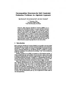
a2 a1
a3
a4
... Figure 1
an
Analysis of robustness. Let us be given a sequence of connected linear intervals a1 = [v0 ,v1 ], a2 = [v1 ,v2 ], ... , an = [vn-1 ,vn ] in an image which forms a linear feature (see Figure 1). We define and compute a relation P on this feature as follows: Let Pi = P(ai , ai+1 ) where P(ai , ai+1 ) = 0 ó D(ai) < D(ai+1 ) and P(ai , ai+1 ) = 1 ó D(ai) ≥ D(ai+1 ) . This relation can be presented as a binary vector, t = (P1 , P2 , P3 , ... , Pk , ... , Pn-1 ) . For example, consider a specific collection of linear intervals that generate a vector t1 =(1,0,1, . . . ). Note that this vector contains information about the relative lengths of successive intervals. For example, t1 states that a1 is no shorter than a2 while a2 is shorter than a3 . Denote the ith component of t1 as t1i . Next, for the purpose of simulation, suppose we apply non- linear transformations to the points that comprise each of the ai intervals. Let a vertex v = (x, y), then the transformed vertex v will be transformed component-wise as v’ = ( f(x, y), g(x, y) ). The relation P would then be recomputed for the transformed intervals. Let t2 = (P’1 , P’2 , P’3 , ... , P’k , ... , P’n-1 ) collect the results of the transformed relation. The vector t2 can then be compared with the vector t1 by computing the Hamming distance H between these vectors: H(t1 , t2 )=Σ k=1,n-1 (t1k -t2k )2 . This distance measures the number of distortions produced by transformations f and g in relation P. If the distance is 0 then the feature is a P-invariant for the (f, g) transformation. Consecutive angles can be treated in a similar way. Let Qi = Q(ai , ai+1 , ai+2 ) where Q(ai , ai+1 , ai+2 ) = 0 ó L(ai , ai+1 ) < L(ai+1 , ai+2 ) , Q(ai , ai+1 , ai+2 ) = 1 ó L(ai , ai+1 ) ≥ L(ai+1 , ai+2 ) and t = (Q 1 , Q2 , Q3 , ... , Qk , ... , Qn-2 ) . As before a transformed vector t2 can then be compared with a vector t1 by computing the Hamming distance H. H(t1 ,t2 )=Σ k=1,n-2 (t1k-t2k )2 . Again this measures the number of distortions in the angles produced by transformations f and g in relation Q and if H is 0 then the feature is called Q-invariant for the (f, g) transformation. Note, all angles are measured consistently.
7. A feature correlating algorithm
We begin this section by presenting a simplified version of an algorithm that finds a maximum co-reference. In essence this algorithm finds the largest n-gram common for two Boolean vectors t1 and t2 . This common n-gram cannot be longer than min(n1 ,n2 ) - H(t1 ,t2 ). There are several known algorithms for finding n- grams with a finite alphabet. In our case, the alphabet is a smallest possible -- {0,1}. Thus, the search is can be relatively fast. At times it may be necessary to consider more than consecutive intervals. Using a notation similar to the previous section, let us denote the angle between ai and ai+1 as Li = L(ai, ai+1 ). Now record in a matrix comparisons between all pairs of angles in a given feature. As above record the i,j entry as 0 iff Li < Lj and 1 iff Li ≥ Lj. Note the resulting matrix is symmetric. Now when two such matrices are built for two features a and b, a more complex approach in determining a maximum co-reference is based on searching for the largest common part these matrices. This is done by “sliding down” the diagonals of the matrices. Consider for example Tables 1 and 2 where the largest common parts are highlighted. Table 1. Illustrative matrix for feature a. Angle L1 L2 L3 L4 L5 L6
L1 1
L2 0 1
L3 1 0 1
L4 1 1 0 1
L5 0 0 1 1 1
L6 1 0 0 0 1 1
Table 2. Illustrative matrix feature b. Angle L1 L2 L3 L4 L5 L6 L7 L8 L9 L10
L1 1
L2 0 1
L3 1 0 1
L4 1 1 0 1
L5 0 0 1 1 1
L6 1 0 0 0 1 1
L7 1 0 1 1 0 1 1
L8 1 0 0 1 0 1 0 1
L9 0 0 0 1 0 0 0 1 1
L10 1 1 1 1 0 0 0 1 1 1
8. Method: an application to conflation
The algorithms described in section 7 are a part of the conflation method. This method includes more components and is based on the following assumptions: 1. A digitized map (e.g. in USGS/NIMA vector format), an aerial photo and SRTM data have no common reference points established in advance for matching them. This is the first source of uncertainty. 2. A map, an aerial photo and SRTM data are made in different (and often) unknown scales, rotations and accuracy. This is the second source of uncertainty. 3. A map, an aerial photo and SRTM data each have as least 5 well-defined linear features that can me presented as polylines (continuos chains of linear intervals). Note, a feature on the map may be only a part of the feature on the aerial photo. Also features might overlap or have no match at all. 4. These well-defined linear features can be relatively easy extracted from a map, an aerial photo and a SRTM data. Major steps of the method: Step 1. Extract a linear feature as a set of points (pixels), S. Step 2. Interpolate this set of points S as a specially designed polyline (see below for more details). Step 3. Construct a matrix P of the relation between all lengths of intervals on the polyline (see below for more details). These matrixes are computed for all available polylines. Step 4. Construct a matrix Q of the relation between all angles on the polyline (see below for more details). These matrixes are computed for all available polylines. Step 5. Search common submatrixes in the set of matrixes P and compute a measure of closeness. Step 6. Search common submatrixes in the set of matrixes Q and compute a measure of closeness. Step 7. Match features using the closest submatrix. Steps 3-6 are a formalization of the calculations presented in section 7. Details. Step 2. A special design of a polyline includes control over the lengths and angles of the linear intervals. For instance, if two adjacent linear intervals have an angle between them “close to” 180o then these intervals would be joined together to form a single interval. Step 3. P={P ij}, where Pij = 1 if the length of ai is greater or equal to the length of aj, Di ≥ Dj and Pij = 0 if the length of ai is greater or equal to the length of aj, Di < Dj. Lengths are defined for all pairs of linear intervals. A more sophisticated version of this step may require the construction of matrices containing first order (and perhaps higher order) differences
between lengths or angles. Additional matrices also can be designed to accommodate specific properties of features (if known) as a set of axioms. Step 4. This step is implemented similar to step 3 -- angles are substituted for the lengths of the linear intervals. Tables 1 and 2 above illustrate steps 4 and 5. Comparison of matrices presented in these tables shows that the first one is a part of the second one. Thus, step 7 (feature matching) can be performed successfully. Examples presented in bkws.pdf file available at ftp://ftp.geology.cwu.edu/pub/sumner/. 9. Related computational topology problems Below we discuss relationship between our task and the tasks discussed in Bern et al. [2]. Shape Reconstruction from Scattered Points is an important part of our algebraic approach. We propose developing a method for reconstructing a linear feature shape using a criteria of maximum of local linearity. Shape Acquisition. Matching/correlating spatial objects requires shape acquisition from an existing physical object. We propose contributing to the solution of this problem by developing a formal mathematical definition of feature such as roads and drainage system as complex objects in terms that coincided with the USGS/NIMA Topological Vector Profile (TVP) Concept. Shape Representation. Bern et al. [2] listed several representation methods: unstructured collections of polygons (“polygon soup”), polyhedral models, subdivision surfaces, spline surfaces, implicit surfaces, skin surfaces, and alpha shapes. The authors conclude that these methods “are at best adequate within their own fields, and not well suited for connecting across fields.” Our contribution to the area would be in developing an algebraic system representation described below, which includes scale-dependent but robust invariants, axioms and permissible transformations. Topology Preserving Simplification. It is critical for many applications to be able to replace a polygonal surface with a simpler one. However, such a process is “notorious for introducing topological errors, which can be fatal for later operations.” [Bern et al, 1999]. We propose using the generic idea developed in Cohen, Varshney, et al. [3] in which a simplified 2-manifold is fitted into a shell around the original. In addition, we propose the development of a specific method for the simplification of linear features critical for the algebraic approach using the similar ideas. Our goal is to enforce algebraic invariants using simplification. The main idea is that the simplification criteria should not be completely defined in advance but be adjusted using extensive simulation experiments and machine learning tools to identify practical limits of robustness of algebraic invariants. It also includes classification of linear features to identify simplification options. Let a is a linear feature, b is its simplification, ? is a measure of the closeness between a and b and ?(a,b) < d, where d is a limit of acceptable simplification. We will develop this limit as an adjustable parameterized function of a feature a, d = d(a).
10. Outline of scope of the research Methods to be employed include presenting properties geospatial objects to be preserved in the generic form of algebraic systems A = 〈 A,P,F〉 where A is a set of objects, P is a set of predicates and F is a set of functions over A and its Cartesian products AxAx…xA. Each such system will be accompanied by a set of axioms that should be satisfied by A. Axioms should be developed for three major conflation categories such as roads and drainage systems. If a road turns with consecutive angles g = 300 and h = 600 then some axioms may require to preserve the property g < h under any permissible transformation f, f(g) < f(h). For transformations that do not preserve such axiom a measure of distortion will be developed and computed for spatial objects. Reverse methods will also be developed and used. Having a value v of the distortion measure these methods will try to reconstruct the transformation T that produced v. This is especially useful for the situation with two unmatched maps M1 and M2 that need to be conflated. Applying T-1 to M1 it is possible to get another map M'1 which can be closer to M2. Applying the same approach to M2 by restoring a transformation R and using R-1 it is possible to get another map M'2 . Finally maps M'1 and M'2 could be made consistent, if T and R were correctly discovered and restored, i.e., T and R actually were used to corrupt maps M'1 and M'2 . 11. Conclusion Matching/correlating similar features from different geospatial databases (conflation problem), and handling approximate and inconsistent data are of great practical importance for end users -defense and intelligence analysts, geologists, geographers, ecologists and others. This papers concludes that a fundamentally new mathematical approach is needed for solving these problems. The paper describes such an approach based on the general concept of an abstract algebraic system. It shows the benefit of developing a fundamentally new algebraic invariants for geospacial data analysis and correlation using such invariants.
References 1.Aronov, B., R. Seidel and D. Souvaine. On compatible triangulations of simple polygons. Comput. Geom. Theory Appl. 3 (1993), 27--35. 2. Bern M. et al, Emerging challenges in computational topology, 1999, citeseer.nj.nec.com/bern99emerging.html 3. Cohen, J., A. Varshney, D. Manocha, G. Turk, H. Weber, P. Agarwal, F.Brooks, Jr., and W. Wright.
Simplification envelopes. In H.Rushmeier, Ed., Proc. SIGGRAPH ’96, 119–128. Addison Wesley, 1996. 4. Dey T., and S. Guha. Computing homology groups of simplicial complexes in _ 3. J.ACM, 45(2):266– 287, March 1998.
5. Dey, T., H. Edelsbrunner, and S. Guha (1999). Computational Topology. In Advances in Discrete and Computational Geometry (Contemporary mathematics 223), ed. B. Chazelle, J. E. Goodman, and R. Pollack, American Mathematical Society, 109--143. http://citeseer.nj.nec.com/dey99computational.html
6. Eppstein D., Geometry in action: Cartography and Geographic Information Systems http://www.ics.uci.edu/~eppstein/gina/carto.html 7. Gillman D., Triangulation for rubber-sheeting, Auto Cartography 7 (1985), 191-197 8. Gupta, H., and Wenger, R. Constructing pairwise disjoint paths with few links. Technical Report OSUCISRC-2/97-TR16, The Ohio State University, Columbus, Ohio, 1997. http://citeseer.nj.nec.com/gupta97constructing.html
9. Mal’cev A.I. Algebraic Systems, Springer-Verlag, New York, 1973.