preliminary results of a dedicated FPGA implementation ... Multi-Level, Monte Carlo, Option Pricing, Heston, GPU, ..... much data between host and device.
Algorithmic Complexity in the Heston Model: An Implementation View Henning Marxen, Anton Kostiuk, Ralf Korn
Christian de Schryver, Stephan Wurm, Ivan Shcherbakov, Norbert Wehn
Stochastic Control and Financial Mathematics Group University of Kaiserslautern Germany
Microelectronic Systems Design Research Group University of Kaiserslautern Germany
{marxen, kostiuk, korn}@ mathematik.uni-kl.de
{schryver, shcherbakov, wehn}@ eit.uni-kl.de,
ABSTRACT
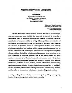
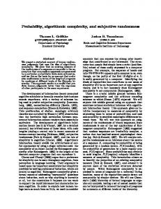
for this is that these models explain observed market prices much better than the famous constant volatility Black-Scholes model [7]. The drawback of advanced stochastic and local volatility models is that they lack closed form price formulae in many cases, especially for exotic options. Thus, numerical methods have to be used. Together with high accuracy requirements, this leads to a dramatic increase of computation time and energy consumption for simulations. Exploiting the speedup and energy saving potential of efficient hardware accelerators is therefore a key to obtain accurate results within short times on the one hand, and to save energy costs on the other hand. In this work, we target the problem of efficient barrier option pricing in the widely applied Heston model [7]. We perform a high-level exploration on application level and show the impact on the important metrics simulation time and energy consumption. From the algorithmic side we employ Monte Carlo methods as they are very robust and applicable to nearly any featured product. Inherently, Monte Carlo methods are wellsuited for parallel execution, and therefore match perfectly to multi-instance hardware accelerators. In 2008, Giles has proposed the so-called multi-level Monte Carlo method [6] that provides better asymptotic convergence. For our paper we therefore consider the multi-level Monte Carlo method in a practical scenario. However, even with the model and the simulation method fixed, a huge design space of all possible algorithmic and implementation parameter selections remains. Figure 1 gives an overview about all the algorithmic varieties considered in this work. The challenge for designing an efficient accelerator implementation is now to select the optimal parameters out of both, the algorithmic and the implementation domain. It is therefore mandatory to consider the effects of selecting a parameter set over both domains simultaneously. We show an optimal algorithm selection in Section 3. The main contributions of this paper are:
In this paper, we present an in-depth investigation of the algorithmic parameter influence for barrier option pricing with the Heston model. For that purpose we focus on singleand multi-level Monte Carlo simulation methods. We investigate the impact of algorithmic variations on simulation time and energy consumption, giving detailed measurement results for a state-of-the-art 8-core CPU server and a Nvidia Tesla C2050 GPU. We particularly show that a naive algorithm on a powerful GPU can even increase the energy consumption and computation time, compared to a better algorithm running on a standard CPU. Furthermore we give preliminary results of a dedicated FPGA implementation and comment on the speedup and energy saving potential of this architecture.
Categories and Subject Descriptors G.3 [Probability and Statistics]: Probabilistic algorithms (including Monte Carlo); G.4 [Mathematical Software]: Algorithm design and analysis
General Terms Algorithms, Design
Keywords Multi-Level, Monte Carlo, Option Pricing, Heston, GPU, Energy, Barrier
1. INTRODUCTION Exotic option pricing is one of the most important numerical problems in computational finance. Nowadays, sophisticated models (for example stochastic and local volatility models) have become industry standards. The reason
• For the practical showcase of multi-level Monte Carlo option pricing with the widely used Heston model, we show that a priori algorithmic investigations are mandatory for the development of efficient accelerators.
Permission to make digital or hard copies of all or part of this work for personal or classroom use is granted without fee provided that copies are not made or distributed for profit or commercial advantage and that copies bear this notice and the full citation on the first page. To copy otherwise, to republish, to post on servers or to redistribute to lists, requires prior specific permission and/or a fee. WHPCF’11, November 13, 2011, Seattle, Washington, USA. Copyright 2011 ACM 978-1-4503-1108-3/11/11 ...$10.00.
• For this application, we provide speed and energy mea-
5
Absorption Plain Barrier Checking Continuity Correction
Reflection
Barrier Checking Non-Negative Volatility
Higham and Mao Partial Truncation Full Truncation
No Variance Reduction
Variance Reduction
Antithetic Variance Reduction
Zhu's Method
Heston Simulation
Monte Carlo Type Plain Simulation Log Asset Simulation
Single-Level Multi-Level
Asset Simulation Type
Figure 1: Selected Algorithm Parameter Set for Barrier Options surement results for CPU and GPU simulations and quantify the potential of GPUs.
For the Black-Scholes model, many FPGA accelerators have been published over the last years. Jin et al. have recently summarized the work and give an overview over different solvers in [8]. However, none of the GPU and FPGA papers so far consider energy aspects. From the algorithmic point of view, there is currently a lack of investigations with respect to the multi-level Monte Carlo method. Lord et al. [10] have introduced the full truncation method in 2010 and compared it with other schemes to avoid negative volatility in the Heston model. Our paper goes further by checking this method with special interest towards barrier options. Furthermore, these methods are combined with more possibilities of simulation choices. A priori it is not clear whether the choice of the method changes if one changes other simulation aspects (see Figure 1). We analyze the effectiveness of the multi-level Monte Carlo method in this context.
• We comment on the impact of selecting an unfitting algorithm for acceleration and on the potential of FPGA acceleration in general. The rest of the paper is structured as follows: Section 2 summarizes related work and the state-of-the-art in research. In Section 3 we give detailed simulation results of the algorithmic variations from Figure 1 and show the impact on the resulting computational complexity. We present the potential of state-of-the-art GPUs for our application and provide run time and energy numbers in Section 4. Together with preliminary results, Section 5 gives an outlook on the massive potential of FPGAs with respect to simulation speedup and energy saving. Section 6 concludes the paper.
2. RELATED WORK
3.
In this section we summarize ongoing work dealing with the acceleration of Heston solvers for the target platforms CPU, GPU and FPGA. Papers presenting Heston pricing on GPUs have appeared recently. Bernemann et al. have highlighted the enormous speedup potential for Monte Carlo based Heston pricing on GPUs, also for multi-underlying simulations on the WHPCF 2010 [1]. For one underlying, they have achieved a speedup factor of 50 in their hybrid CPU/GPU setup, compared to CPU only simulations. Using the COS method that is based on Fourier cosine series expansions, Zhang and Oosterlee have investigated several workload splits in a hybrid CPU/GPU setup in 2010 [13]. They have shown that they can profit most from the GPU if most of the arithmetic operations on the high numbers of paths can be performed on the GPU. We have used a similar partitioning scheme for our multi-level Monte Carlo GPU implementation in Section 4. Bernemann et al. have enhanced their WHPCF paper [1] with more measurement data in February 2011 [2]. They also included a comparison of two different random number generation approaches: Using pseudo random numbers in the Monte Carlo simulations, they achieve a speedup of up to 50 compared to CPU only simulations. For Sobol Brownian bridge quasi random number generation, the GPU speedup is decreased by around 30%. To the best of our knowledge, no publications showing FPGA option pricing accelerators based on the Heston model exist up to now, despite the high potential of FPGAs for speedup and energy saving in high performance computing.
ALGORITHMIC ASPECTS
The Heston model has been introduced in 1993 [7] and has advanced to an industry standard nowadays. The model itself consists of two stochastic differential equations (SDEs) that describe the dynamic of the asset price S (Equation 1) and the volatility V of the asset price (Equation 2). √ (1) dS(t) = rS(t)dt + V (t)S(t)dW1 (t) √ dV (t) = κ(θ − V (t))dt + σ V (t)dW2 (t) (2) Note that the two driving Brownian motions W1 and W2 are correlated. While approximating the solution of a stochastic differential equation, an error usually appears. The error of a stochastic estimation can be measured by the mean squared error (MSE), which is the expected squared difference of the approximated and the exact value. The MSE can be divided into two distinct sources of error. One part is the variance of the estimation, sometimes called the stochastic error, and the second is the bias, or also called the systematic error, from the discretization of the continuous SDE. M SE = V ariance + (Bias)2
(3)
Both error sources are independent from one another. In order to reduce the variance, more simulations have to be conducted. The bias is not impacted by this, but can be reduced by increasing the discretization steps in the simulations. In 2008, Mike Giles has introduced the so called multilevel Monte Carlo method [6]. With respect to asset price simulations, the idea is to simulate the price paths not only
6
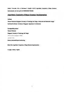
on a fine level with many discretization steps, but also on a coarser one simultaneously. The term level defines a discretization with a specific number of discretization steps. A higher level means a finer discretization. We use a multilevel constant of 4, see [6] for further details. Figure 2 shows the two discretizations of the same path of a stochastic differential equation. Giles has proven that the convergence of this scheme is much better, and for a high precision it will outperform the single-level Monte Carlo scheme. In this paper we consider the special case of barrier options in the Heston model and investigate the method for its practical use.
able, it is impossible to reproduce or meaningfully interpret the results. We therefore have suggested a benchmark set to be able to fairly compare different algorithms and their implementations [4], which is available online1 . It consists of a collection of different numbered market scenarios from the literature. They span a wide range of parameters that are observable in real markets. For the payoff, the focus lies on European knock-out double barrier options, but also different option types are included.
3.2
125
120
115
Asset Price
Behavior of the Systematic Error
The systematic error in Equation 3 is the absolute value of the difference of the expectation of the payoff of the discretized process and the expectation of the payoff of the original continuous process. This error is caused only by the discretization of the SDE. Besides the number of time steps, several more parameters from Figure 1 influence the total discretization scheme: • negative volatility treatment
110
• asset simulation type
105
• barrier checking 100
95 0
0.2
0.4
0.6
0.8
In order to calculate the systematic error, the correct solution to the SDE – or a very good approximation of it – is needed. The expected value of the discretized process is in general unknown and needs to be approximated. In this paper we focus on the single- and the multi-level Monte Carlo method. The systematic error is the same for both schemes as they are based on the same discretization schemes [6].
1
Time
Figure 2: A Continuous Asset Price and Two Different Discretizations Using 4 and 16 Discretization Steps (Corresponds to Level 1 and 2 Respectively). The variance can usually be calculated during the simulation. Therefore the stochastic error can be estimated and controlled quite precisely. In contrast to the variance, the bias can not be calculated directly and is usually only appraised. However, by using the multi-level Monte Carlo algorithm a reasonable estimate for the bias can be obtained. This estimate is not as exact as the approximation of the stochastic error. See [6] for further details. One difficulty arises in the discretized variance process. The continuous process is always non-negative, but the discretized process can become negative if not dealt with accordingly. The way to circumvent the possibility of a negative variance process is one striking difference between the considered algorithms. For more details see [10] and [14]. Even though one would expect that the behavior of the discretized variance process around the origin is insignificant, it turns out this is not the case, see Section 3.2. In the following analysis, firstly the two error sources will be treated separately. Afterwards we show the influence of the combined sources to the overall computational complexity in two characteristic test cases.
3.2.1
Negative Volatility Treatment
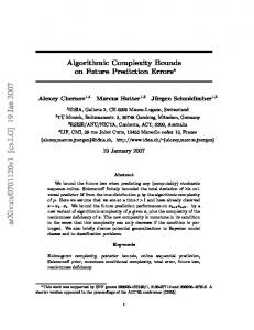
Lord et al. state in [10] that the full truncation scheme is the best Euler scheme for the pricing of European vanilla options in the Heston setting. Figure 3 exemplifies this behavior. We can see that the convergence of the full truncation scheme is better than that of the absorption scheme and simulating the log asset price increases the accuracy even more. The test case is case 1 of the benchmark. In this setting, the full truncation scheme is superior to the other tested schemes. In the case of double barrier options, this behavior is similar but not exactly the same. In a few cases (5,8,9) of the benchmark, the difference between the simulation schemes is negligible. Figure 4(a) shows the behavior of the systematic error with the absorption, the partial truncation and the full truncation scheme. However, in several tested cases the difference is huge and in fact hardly any convergence can be seen for the absorption scheme (3,4,6,12). This is the case for the test parameter set 4 of the benchmark, plotted in Figure 4(b). Higham and Mao and the reflexion scheme also fail to show a convergence in a several cases (3,4,6,12). We can see the partial truncation scheme is similar or even a bit better than the full truncation scheme. These observations suggest to take the full or the partial truncation scheme for option pricing applications.
3.1 The Test Setting Comparing different algorithms with various implementations on different architectures is a difficult task. During our research we have seen many publications in our field, presenting elaborate new designs. Most authors evaluate their work by giving results for architecture specific metrics (like area consumption) or the speedup compared to a software implementation. As this implementation is often not avail-
1
7
http://www.uni-kl.de/benchmarking
100
1
absorption partial truncation full truncation
absorption partial truncation full truncation
systematic error |EYl - EY|
systematic error |EYl - EY|
10
100
-1
10
10-2
1
4
16
64
256
1024
10-1
10-2 1
4096
16
4
Discretization Steps
64
256
1024
4096
Discretization Steps
(a) Case 8, No Significant Difference
(b) Case 4, Significant Difference
Figure 4: Different Behavior of the Non-Negative Volatility Algorithms 101
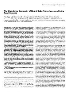
the continuity correction decreases the accuracy for coarse discretizations. This is due to the fact that the barrier correction of the upper and lower barrier can meet for a big time step. This is not a problem for finer discretizations anymore. Therefore it is even more important to carefully choose the (finest) discretization.
absorption full truncation log full truncation
0
-1
10
1
10
asset simulation log asset simulation log asset simulation with barrier correction
10-2
100 10
systematic error |EYl - EY|
systematic error |EYl - EY|
10
-3
-4
10
1
4
16
64
256
1024
4096
Discretization Steps
Figure 3: The Systematic Error in a Vanilla European Call Setting (1).
-1
10
10-2
10-3
10-4
3.2.2 Asset Simulation Type
10-5
1
4
16
64
256
1024
4096
Discretization Steps
It is not obvious what the affect of simulating the log asset price is. In the simpler Black-Scholes setting (with a constant volatility), simulating the log asset there is no bias (of one time step) at all. Here the two simulation types are very similar. In most cases it improves the result at the 0th and 1st level quite well and for bigger levels there is no big difference with or without it. This effect is the same for the absorption and the full truncation scheme.
Figure 5: Influence of the Continuity Correction on the Systematic Error (Case 8).
3.2.4
Parameter Interactions
It is worth mentioning that the simulation of the log asset is essential for a fast use of the continuity correction scheme. The correction term is just added in the case of the log asset price, whereas in the case of simulating the asset price itself, an exponential function needs to be calculated in order to obtain the multiplier to change the barrier. As this needs to be done in each time step and for each simulation separately, this significantly slows down the process. Seeing this, there is a good reason to use the log asset price. We have simulated and observed the different variance simulation schemes again with log asset simulation and continuity correction. The result is not exactly the same as in the case of the direct asset simulation. Comparing the full truncation scheme with the other schemes (absorption, reflection, Higham and Mao, and partial trun-
3.2.3 Barrier Checking The convergence of the systematic error increases drastically by introducing the continuity correction of the barrier. Broadie, Glasserman and Kou [3] introduced a continuity correction in the Black-Scholes setting. To apply it in the Heston setting, we use the current volatility. Figure 5 shows the comparison of an asset simulation without continuity correction, a log asset simulation without continuity correction and a log asset simulation with continuity correction. In all considered cases the asset and the log asset simulation are similar and the introduction of the continuity correction increases the order of convergence significantly. In some cases,
8
cation), full truncation has the smallest bias in most tested cases. This is in contrast to the simpler case where the partial truncation scheme performed slightly better than full truncation. Nevertheless, partial truncation has a similar convergence as the full truncation scheme, whereas all other schemes have problems with several of the test situations and hardly any convergence can be seen in these cases. Taking Zhu’s method with log asset simulation in the comparison, the observation is similar to the absorption scheme. Even though in a few cases (1,5) it performs better than the latter one, in several situations (3,4,6,12) hardly any convergence can be seen.
systematic and stochastic error on two showcases, that are case 4 and case 5 of our benchmark set [4]. We define computational complexity (CC) as the total number of discretization steps to be computed over all simulated paths. One simulation with the antithetic variance reduction has two paths, the original path and the antithetic path. Thus the number of time steps per simulation are twice the number of discretization steps. We return to the task of bounding the root mean squared error (MSE). In our case of double barrier options, the analysis of the last two sections suggests to use the log asset simulation and for the variance process the full truncation scheme. To account for the discrete observed barrier, use the barrier correction technique. Furthermore we suggest to use antithetic variance reduction to increase the speed even more. We call this the suggested algorithm and show how it performs compared to other schemes.
3.3 Behavior of the Variance Concerning the variance, the simulation shows a different behavior. Looking at the different discretization schemes, we see that the full truncation scheme has in many cases a higher variance than the absorption method. This is the case in the simple asset simulation as well as in the case of log asset simulation with boundary correction and antithetic variance reduction. The other schemes are in between. In the case of antithetic variance reduction, two correlated paths are simulated simultaneously. The variance for the mean of two independent paths is half the variance of one path. Thus to account for the higher number of simulations in the antithetic case, the variance is multiplied by two. Even after this adjustment, we can see the improvement from the simple antithetic variance reduction. In the multi-level setting, the variance is not reduced significantly by antithetic variance reduction. It is about the same as simulating two paths. However, simulating one path and the antithetic path can be faster than computing two independent paths (see Section 4). Another surprising observation is that in half of the tested cases the multi-level variance is above the single-level variance (at least up to level 6). One would expect to have a lower variance. Therefore the need to carefully choose when to use the multi-level method arises. The difficulty can also be avoided by choosing an optimal start level for the multilevel algorithm. In several situations, even for moderate root MSE ϵ the final level has to be bigger than 6 in order to achieve a bias that is small enough. In fact, in further testing it can be seen that, as expected, the variance decreases further for increasing levels and is lower than the single-level variance for higher levels. Another interesting observation can be made in connection with the barrier correction. Once we have introduced the continuity correction into our simulations (keeping everything else the same), the variance in the multi-level case drops significantly. As seen, introducing the continuity correction decreases the difference between two consecutive levels. As the value is decreased the variance is also decreased. However the variance is not decreased in the same way the expected value is. Thus we can observe a relative high variance compared to a low expected value. Even without the continuity correction in the multi-level case, we have a high standard deviation relative to the expected values.
3.4.1
First Showcase (Benchmark Case 4)
The first example is case 4 from our benchmark [4]. We look at a double barrier knock-out option in the Heston model. In this particular case an analytical solution exists, therefore we can provide the bias of the simulation with a high precision. Table 1 shows the bias, the variance, and the multi-level variance up to level 6. The three schemes considered are the simplest method (the absorption scheme) and two more sophisticated ones: the full truncation scheme with antithetic variance reduction only and the suggested algorithm. The rounded true value in this situation is 0.74870. The root MSE is bounded by 0.03. In order to achieve this we bound the variance to be less than 21 0.032 and the bias to be √ 1 less than 0.03. See Equation 3 for more details. Using 2 the absorption scheme, one would have to simulate on a very high level bigger than 6. In fact even on level 10 (with more than one million time steps) the bias is approximately 0.12. Thus we will not consider it in our computations. With the full truncation scheme we need 3139 simulations on level 6. Thus we have to compute 3139 ∗ 2 ∗ 46 ≈ 2.57 ∗ 107 time steps. Using full truncation with log asset simulation and continuity correction it is enough to simulate 3386 simulations on level 3. Thus we have to compute approximately 4.33 ∗ 105 time steps. So the suggested algorithm is better than the plain full truncation asset simulation by a factor of 59.3. It is obvious that the multi-level algorithm does not yield any help in this, as the multi-level variance is bigger or not significantly smaller than the single-level variance for all schemes and all observed levels. An algorithm to determine the optimal start level of the multi-level algorithm should result in using the single-level scheme in this particular case, that means start with the finest level you want to simulate.
3.4.2
Second Showcase (Benchmark Case 5)
The second example is case 5 of the benchmark set. Here, the multi-level method can decrease the computational complexity even for reasonable required precisions of the estimation. Comparing Table 3 with Table 1, we see that the behavior is different from that in Section 3.4.1. The full truncation scheme has a bias that is similar to the one of the absorption scheme. The lower variance mainly results from the antithetic variance reduction. The suggested scheme
3.4 Combining the Results This section underlines the importance of the choice of the algorithm and its impacts on the resulting computational complexity. We show the influence of the combined
9
level 0 1 2 3 4 5 6
absorption scheme bias variance ML var 5.2798 0.1878 0.1403 3.4021 7.7865 0.2230 2.7565 5.1466 0.2367 2.5360 4.0242 0.2258 2.4765 3.2023 0.2153 2.4579 2.5842 0.1911 2.5204 2.1152
full truncation scheme bias variance ML var 2.2186 0.1909 0.0534 2.1523 4.0896 0.1910 2.0690 3.6303 0.1260 1.7072 2.7964 0.0662 1.5391 2.1725 0.0369 1.4573 1.8025 0.0181 1.4124 1.5553
suggested algorithm bias variance 1.0496 0.3820 0.2102 1.3700 0.0401 1.5236 0.0086 1.3991 0.0043 1.3712 0.0006 1.3692 0.0005 1.3677
(see 3.4) ML var 2.3320 2.5338 2.2039 1.8731 1.6621 1.4963
Table 1: Bias and Variance of the Different Schemes scheme CC in time steps CC / best CC
absorption single-level multi-level not possible not possible
full truncation scheme single-level multi-level 2.57 ∗ 107 single-level 59.3 single-level
suggested algorithm (see 3.4) single-level multi-level 4.33 ∗ 105 single-level 1 single-level
Table 2: Computational Complexity for Different Schemes with a Precision of 0.03
4.
has a significantly lower bias. In this setting the multi-level variance on the higher levels is a considerable lower than the single-level variance. Therefore the multi-level scheme reduces the computational complexity for a high enough end level. The rounded value √is 5.7576 and we allow a root MSE of 1 0.2 and a variance of 21 0.22 . 0.2, a bias of up to 2 In both the absorption and the full truncation scheme, we have to simulate on level 6. In the first scheme we need 3342 simulations, in the latter case 1521. Thus we need to compute 1.37 ∗ 107 and 1.25 ∗ 107 time steps respectively. Remember that the full truncation scheme used here has antithetic variance reduction. Therefore the computational complexity per path is twice the discretization steps. In doing so we see that the full truncation scheme is slightly better. Furthermore, it is faster to compute one simulation and the corresponding antithetic variate than two independent simulations. See Section 4 for more details on this. By using the full truncation scheme with continuity correction to simulate the log asset the bias is a lot lower. In this case it is sufficient to simulate 1481 simulations on level 2. Thus we need to simulate 4.74 ∗ 104 time steps. For the first two schemes, we can use the multi-level Monte Carlo algorithm with start level 4 to achieve a better computational complexity as the single-level scheme. We have a computational complexity of 7.56 ∗ 106 and 7.31 ∗ 106 respectively. For the suggested algorithm from Section 3.4, it is not useful to use the multi-level algorithm if we simulate only up to level 2. The optimal start level is 4 as in the other case, that means use single-level Monte Carlo for computations up to and including level 4 and for a higher precision start the multi-level method from level 4. The higher the end level is, the higher is the benefit of the multi-level scheme. In this section we have compared the different algorithmic aspects independently of a possible implementation. We have analyzed the impact on the systematic and stochastic error and suggested an algorithm to use for the pricing of barrier options in the Heston model with the Monte Carlo simulation. For two selected test cases, we have pointed out the immense difference of the algorithms on the computational complexity. In the next section we will show that bringing a naive algorithm to a hardware accelerator can even be less efficient than the suggested algorithm in a simple CPU implementation.
IMPLEMENTATION ASPECTS
Starting from the existing CPU benchmark, we have created an equivalent implementation with GPU acceleration. To support as many as possible hardware architectures, we have decided to use OpenCL instead of the commonly used CUDA to interface with the GPU. In the following sections we briefly describe the GPU implementation and compare the simulation results.
4.1
GPU Acceleration
Our benchmark system consists of a Intel Xeon W3550 server with eight cores running at 3.07GHz, 8GB of RAM and OpenSuSE 11.4 64 bit. The general purpose graphic processing unit (GPGPU) used for all benchmarks is a Nvidia Tesla C2050 with driver version 270.41.06 from April, 20th 2011 installed, supporting OpenCL 1.0. The C++ software reference model has been compiled with GCC 4.5.1 without any specific compiler flags set. As already mentioned in Section 2, Zhang and Oosterlee have discovered best performance results when locating most of the algorithm on the GPU [13]. Therefore we have used a similar partitioning in our work. Random number generation, path simulation and barrier checking are completely executed on the GPU without the need to exchange much data between host and device. For the pricing, we have chosen a hybrid approach with both CPU and GPU involved. To allow fair energy comparisons with the serveronly implementation, the simulation control itself remains on the host, where it generates only small load on one core. The Monte Carlo simulation described in Section 3 depends on a high amount of (pseudo) random numbers. These are generated in two steps: The first step is to produce uniformly distributed random numbers. For this purpose we have ported the Mersenne Twister for Graphic Processors (MTGP) [12] to OpenCL. In the second step we use Acklam’s inverse normal cumulative algorithm [11] to convert those numbers to normally distributed ones.
4.2
Accelerating a Naive Algorithm
Up to now, we have compared the different algorithmic flavors using the notion of computational complexity in the sense of number of discretization steps. Now, we use the GPU implementation to compare real-time data. Table 5 shows the overhead in time of the different simulation methods. The figures are taken from the simulation on the GPU.
10
level 0 1 2 3 4 5 6
absorption scheme bias variance ML var 86.748 1.8851 1.5283 82.385 83.887 0.9372 75.270 71.393 0.5436 71.166 37.011 0.2891 68.620 18.009 0.1604 67.420 8.6848 0.0826 66.831 4.4077
full truncation scheme bias variance ML var 27.405 1.8675 2.1290 36.458 43.120 1.2270 33.855 38.795 0.6202 32.083 20.090 0.3126 31.180 9.3731 0.1523 30.655 4.4823 0.0767 30.408 2.1567
suggested algorithm bias variance 23.011 1.3384 0.4746 28.667 0.0889 29.605 0.0234 29.976 0.0082 30.088 0.0046 30.125 0.0033 30.137
(see 3.4) ML var 37.575 31.667 18.485 8.9906 4.3258 2.1155
Table 3: Bias and Variance of the Different Schemes scheme CC in time steps CC / best CC
absorption single-level multi-level 1.37 ∗ 107 7.56 ∗ 106 289 159
full truncation scheme single-level multi-level 1.25 ∗ 107 7.31 ∗ 106 263 154
suggested algorithm (see 3.4) single-level multi-level 4.74 ∗ 104 single-level 1 single-level
Table 4: Computational Complexity for Different Schemes with a Precision of 0.2 As expected, the difference in speed of the various methods to avoid a negative variance is negligible. In our tests the difference was less than 3% and may also be due to the stochastic nature of the calculation. Introducing the logarithmic simulation did not change the speed much, for more than 16 discretization steps. In this case the overhead was less than 7%. As most of the calculation will be done on finer levels, this is most important. The antithetic variance reduction slows down the process considerably. However, it is still faster than simulating two independent paths and thus useful as seen in Section 3.3. The impact on the computation speed of the barrier correction is also not that big compared to the improvements in convergence. Speed difference to fastest scheme various methods to avoid negative volatility logarithmic calculation antithetic variance reduction introducing the barrier correction
Therefore we see that the algorithmic choice has a significant impact on the computation speed and energy consumption. The algorithm chosen for acceleration should therefore be evaluated very carefully in advance. For pricing barrier options in the Heston model, we recommend to use the suggested algorithm from Section 3.4, since it provides the best performance.
4.3
In the previous section we have shown how important the right choice of the algorithm is. Now we provide runtime and energy measurement results and compare CPU and GPU implementations of the suggested algorithm from Section 3.4. Table 7 shows the comparison of this algorithm running on the server and on the GPU (see Section 4). The time and the energy consumption is given. Due to the architecture of the GPU, the speedup increases with the number of simulations. Thus, for only a few simulations the speedup is around 4. At the same time, the GPU implementation consumes only less than half of the energy compared to the CPU. For a higher demanded precision (and therefore also more parallel paths to simulate) the speedup goes up to a factor of 7 while being 4 times more energy efficient. This behavior is the same for all cases of the benchmark. Table 7 exemplifies this for case 4. So especially for precise calculations, significant speedups and energy savings can be achieved by using the GPU implementation instead of simulating on a standard CPU server.
< 3% < 7% 40% − 60% 5%
Table 5: Calculation Time Overhead of the Different Schemes To illustrate again the impact of the algorithm, we compare the hardware accelerated GPU implementation of the plain simulation scheme (that is asset price simulation and the absorption scheme for the variance process without barrier correction or antithetic variance reduction) with the suggested algorithm running on 1 core of the server. The setting is case 5 as presented above. The required precision was 0.01. Even if running on only one core of our test system, the suggested algorithm from Section 3.4 is almost 7 times faster than the hardware accelerated plain algorithm on the GPU. Table 6 shows that the energy consumption is also well below it. Making use of all 8-cores would increase both, speed and also energy efficiency, significantly.
Computational Time in s Energy Consumption in kJ
Server (1 Core) 24.51 2.6
Real-Time Comparison
5.
CURRENT AND FUTURE WORK
In order to investigate additional energy saving and speedup potential of FPGAs, we are currently developing an equivalent hardware implementation of the suggested algorithm from Section 3.4. For the random number generation, we use a Tausworthe88 uniform random number generator [9] and our inversion based converter from 2010 [5]. The final pricing is only executed once at the very end of the simulation, and therefore remains on a host system connected via USB to the FPGA board. We provide preliminary synthesis results for the latest Xilinx Virtex-7 FPGA series (device xc7v2000tl, package flg1925, speed -2) in Table 8. The Xilinx XPower Analyzer gives a total chip power estimation of 1.038 W. From Table 8 we see that the critical resources are the
GPU 165.83 51.4
Table 6: Comparison of a Hardware Accelerated Naive Algorithm With the Suggested Algorithm Running on a Single Core
11
precision 0.01 0.005 0.001
time (in s) 0.19 0.61 226.23
8-core CPU energy consumption (in J) 35 113 42079
time 0.05 0.11 32.37
Tesla GPU energy consumption 15 34 10034
improvement of GPU over CPU speedup factor energy saving factor 3.76 2.25 5.57 3.34 6.98 4.19
Table 7: Comparison of the Throughput and Energy Consumption of the CPU and GPU Implementation
Slices LUTs Flip-Flops DSP48E1 slices BRAM36 slices Max. frequency
Number 2,393 6,212 7,425 39 6 104 MHz
Percentage 0.8% 0.5% 0.3% 1.8% 0.5%
[2] A. Bernemann, R. Schreyer, and K. Spanderen. Accelerating Exotic Option Pricing and Model Calibration Using GPUs, Feb. 2011. [3] M. Broadie, P. Glasserman, and S. Kou. A continuity correction for discrete barrier options. Math. Finance, 7(4):325–349, 1997. [4] C. de Schryver, M. Jung, N. Wehn, H. Marxen, A. Kostiuk, and R. Korn. Energy Efficient Acceleration and Evaluation of Financial Computations towards Real-Time Pricing. In A. K¨ onig, A. Dengel, K. Hinkelmann, K. Kise, R. Howlett, and L. Jain, editors, Knowledge-Based and Intelligent Information and Engineering Systems, volume 6884 of Lecture Notes in Computer Science, pages 177–186. Springer Berlin / Heidelberg, 2011. [5] C. de Schryver, D. Schmidt, N. Wehn, E. Korn, H. Marxen, and R. Korn. A New Hardware Efficient Inversion Based Random Number Generator for Non-Uniform Distributions. In Reconfigurable Computing and FPGAs (ReConFig), 2010 International Conference on, pages 190–195, Dec. 2010. [6] M. B. Giles. Multilevel Monte Carlo path simulation. Operations Research-Baltimore, 56(3):607–617, 2008. [7] S. L. Heston. A Closed-Form Solution for Options with Stochastic Volatility with Applications to Bond and Currency Options. Review of Financial Studies, 6(2):327, 1993. [8] Q. Jin, W. Luk, and D. B. Thomas. On Comparing Financial Option Price Solvers on FPGA. In Field-Programmable Custom Computing Machines (FCCM), 2011 IEEE 19th Annual International Symposium on, pages 89 –92, May 2011. [9] P. L’Ecuyer. Maximally Equidistributed Combined Tausworthe Generators. Mathematics Of Computation, 65(213):203–213, Jan. 1996. [10] R. Lord, R. Koekkoek, and D. van Dijk. A comparison of biased simulation schemes for stochastic volatility models. Quantitative Finance, 10(2):177–194, 2010. [11] NVIDIA corp. OpenCL SDK code samples. http://developer.nvidia.com/ opencl-sdk-code-samples. [12] M. Saito. A Variant of Mersenne Twister Suitable for Graphic Processors. CoRR, abs/1005.4973, 2010. [13] B. Zhang and C. W. Oosterlee. Acceleration of Option Pricing Technique on Graphics Processing Units. Technical Report 10-03, Delft University of Technology, Feb. 2010. [14] J. Zhu. A Simple and Exact Simulation Approach to Heston Model. SSRN eLibrary, July 2008.
Table 8: Synthesis Results for Virtex-7 FPGA DSP48E1 slices used in the floating point units. This means that around 50 instances of the current accelerator design could be mapped onto one device, all running in parallel. Especially with respect to energy saving, but also for speed, we therefore expect a benefit of at least two decades from using FPGAs over CPU or GPU based Heston pricers.
6. CONCLUSION For the practical application of pricing double barrier options with the industry standard Heston model, we have presented a comprehensive algorithmic analysis for several multi-level Monte Carlo simulation algorithms. The investigations include state-of-the-art barrier checking and variance reduction methods, as well as several approaches for treating non-negative volatility in the discretization scheme. To obtain comparable metrics, we have applied a unified benchmark set for option pricing with the Heston model consisting of a number of market relevant settings. From this analysis, we have identified a specific algorithmic flavor that performs best in nearly all cases and that we suggest to use for the acceleration. By giving precise numbers, we have highlighted how important the selection of a performant algorithm is for efficient acceleration of this problem on GPUs and FPGAs. Furthermore, we have shown that for accelerating the suggested algorithm with a desired precision of 0.001 on the GPU, we achieve a improvement of nearly 7 in simulation time and reduce the energy consumption by a factor of 4 at the same time. We have given preliminary results for a dedicated FPGA implementation and have underlined the immense potential of this platform for speedup and energy reduction for the considered application.
Acknowledgment We gratefully acknowledge the partial financial support from the Center of Mathematical and Computational Modeling (CM)2 of the University of Kaiserslautern. Furthermore, we give special thanks to Laurin de Schryver for putting his birth on the shelf until the paper was finished.
7. REFERENCES [1] A. Bernemann, R. Schreyer, and K. Spanderen. Pricing Structured Equity Products on GPUs. In High Performance Computational Finance (WHPCF), 2010 IEEE Workshop on, pages 1 –7, Nov. 2010.
12