ALGORITHMIC COMPUTATION OF POLYNOMIAL AMOEBAS D. V. Bogdanov1 , A. A. Kytmanov2 , and T. M. Sadykov3
arXiv:1604.03603v1 [cs.CG] 12 Apr 2016
1
Plekhanov Russian University 125993 Moscow, Russia
[email protected] 2
Siberian Federal University
Svobodny 79, Krasnoyarsk, 660041, Russia
[email protected] 3
Plekhanov Russian University 125993 Moscow, Russia
[email protected]
Abstract. We present algorithms for computation and visualization of amoebas, their contours, compactified amoebas and sections of three-dimensional amoebas by two-dimensional planes. We also provide a method and an algorithm for the computation of polynomials whose amoebas exhibit the most complicated topology among all polynomials with a fixed Newton polytope. The presented algorithms are implemented in computer algebra systems Matlab 8 and Mathematica 9. Keywords: Amoebas, Newton polytope, optimal algebraic hypersurface, the contour of an amoeba, hypergeometric functions
1
Introduction
The amoeba of a multivariate polynomial in several complex variables is the Reinhardt diagram of its zero locus in the logarithmic scale with respect to each of the variables [16]. The term «amoeba» has been coined in [5, Chapter 6] where two competing definition of the amoeba of a polynomial have been given: the affine and the compactified versions. Both definitions are only interesting in dimension two and higher since the amoeba of a univariate polynomial is a finite set that can be explored by a variety of classical methods of localization of polynomial roots.
The geometry of the amoeba of a polynomial carries much information on the zeros of this polynomial and is closely related to the combinatorial structure of its Newton polytope (see Theorem 1). Despite loosing half of the real dimensions, the image of the zero locus of a polynomial in the amoeba space reflects the relative size of some of its coefficients. From the computational point of view, the problem of giving a complete geometric or combinatorial description of the amoeba of a polynomial is a task of formidable complexity [10], despite the substantial recent progress in this direction [12,13,11]. The number of connected components of an amoeba complement as a function of the coefficients of the polynomial under study is still to be explored by means of the modern methods of computer algebra. In particular, the conjecture by M.Passare on the solidness of maximally sparse polynomials (see Definition 5) remains open for a long time. Amoebas can be computed and depicted by means of a variety of approaches and methods (see [3,10,8,12,6,13] and the references therein). The present paper is meant to move forward the art of computing and drawing complex amoebas of algebraic hypersurfaces. A special attention paid to the geometrically most interesting and computationally most challenging case of optimal hypersurfaces (see Definition 4). We expose methods and algorithms for computation and visualization of amoebas of bivariate polynomials, their contours and compactified versions. The developed algorithms are used in higher dimensions for depicting sections of amoebas of polynomials in three variables. The main focus of the paper is on polynomials whose amoebas have the most complicated topological structure among all polynomials with a given Newton polytope (see Definition 4). We provide an algorithm for explicit construction of such polynomials. The presented algorithms are implemented in the computer algebra systems Matlab 8 (64-bit) and Wolfram Mathematica 9 (64-bit). All examples in the paper have been computed on Intel Core i5-4440 CPU clocked at 3.10 GHz with 16 Gb RAM under MS Windows 7 Ultimate SP1.
2
CONVEX POLYTOPES, CONES AND AMOEBAS: DEFINITIONS AND PRELIMINARIES
Let 𝑝 (𝑥) be a polynomial in 𝑛 complex variables: 𝑝 (𝑥1 , . . . , 𝑥𝑛 ) =
∑︁ 𝛼∈𝐴
𝑐𝛼 𝑥 𝛼 =
∑︁ 𝛼∈𝐴
𝛼𝑛 1 𝑐𝛼1 ...𝛼𝑛 𝑥𝛼 1 · . . . · 𝑥𝑛 ,
where 𝐴 ⊂ Z𝑛 is a finite set. Definition 1. The Newton polytope 𝒩𝑝(𝑥) of a polynomial 𝑝 (𝑥) is the convex hull of the set 𝐴 of its exponent vectors. Definition 2. The recession cone of a convex set 𝑀 is the set-theoretical maximal element in the family of convex cones whose shifts are contained in 𝑀 . Definition 3. The amoeba 𝒜𝑝(𝑥) of a polynomial 𝑝 (𝑥) is the image of its zero locus under the map Log : (𝑥1 , . . . , 𝑥𝑛 ) ↦−→ (ln |𝑥1 | , . . . , ln |𝑥𝑛 |) . The connected components of the complement to the amoeba 𝒜𝑝(𝑥) are convex and in bijective correspondence with the expansions of the rational function 1/𝑝(𝑥) into Laurent series centered at the origin [4]. The next statement shows how the Newton polytope 𝒩𝑝(𝑥) is reflected in the geometry of the amoeba 𝒜𝑝(𝑥) [4, Theorem 2.8 and Proposition 2.6]. Theorem 1. (See [4].) Let 𝑝 (𝑥) be a Laurent polynomial and let {𝑀 } denote the family of connected components of the amoeba complement 𝑐𝒜𝑝(𝑥) . There exists an injective function 𝜈 : {𝑀 } → Z𝑛 ∩ 𝒩𝑝(𝑥) , such that the cone that is dual to the polytope 𝒩𝑝(𝑥) at the point 𝜈 (𝑀 ) coincides with the recession cone of 𝑀 . In particular, the number of connected components of 𝑐𝒜𝑝(𝑥) cannot be smaller than the number of vertices of the polytope 𝒩𝑝(𝑥) and cannot exceed the number of integer points in 𝒩𝑝(𝑥) . Thus the amoeba of polynomial 𝑝(𝑥) in 𝑛 > 2 variables is a closed connected unbounded subset of R𝑛 whose complement consists of a finite number of convex connected components. Besides, a two-dimensional amoeba has «tentacles» that go off to infinity in the directions that are orthogonal to the sides of the polygon 𝒩𝑝(𝑥) (see Fig. 3.1, 3.2, 4.1). The two extreme values for the number of connected components of an amoeba complement are of particular interest. Definition 4. (See [4, Definition 2.9].) An algebraic hypersurface ℋ ⊂ (C* )𝑛 , 𝑛 > 2, is called optimal if the number of connected components of the complement of its amoeba 𝑐𝒜ℋ equals the number of integer points in the Newton polytope of the defining polynomial for ℋ. We will say that a polynomial (as well as its amoeba) is optimal if its zero locus is an optimal algebraic hypersurface.
In other words, an algebraic hypersurface is optimal if the topology of its amoeba is as complicated as it could possibly be under the condition that the Newton polytope of the defining polynomial is fixed. The other extreme case of the topologically simplest possible amoeba is defined as follows. Definition 5. (See [9].) An algebraic hypersurface ℋ ⊂ (C* )𝑛 , 𝑛 > 2, is called solid, if the number of connected components of its amoeba complement 𝑐𝒜ℋ equals the number of vertices of the Newton polytope of its defining polynomial ℋ. Thus the solid and the optimal amoebas are the endpoints of the spectrum of amoebas of polynomials with a given Newton polytope. Of course there exist plenty of optimal (as well as solid) amoebas defined by polynomials with a given Newton polytope. In fact, both sets of amoebas regarded as subsets in the complex space of coefficients of defining polynomials, have nonempty interior. In the bivariate case, an amoeba is solid if and only if all of the connected components of its complement are unbounded and no its tentacles are parallel. A two-dimensional optimal amoeba has, on the contrary, the maximal possible number of bounded connected components in its complement and the maximal possible number of parallel tentacles. The functional dependency of the topological type of the amoeba 𝒜𝑝(𝑥) on the coefficient of its defining polynomial 𝑝 (𝑥) is complex and little understood at the present moment. A sufficient condition for the amoeba of a polynomial to be optimal is that it satisfies a «natural» system of partial differential equations of hypergeometric type [1,2] while the support of the polynomial in question is complex enough [14]. In Section 4 we expose an algorithm for the computation of the hypergeometric polynomial with the prescribed Newton polytope. Example 1. Let 𝒩 denote the convex hull of the set of lattice points {(0, 0) , (1, 0) , (0, 2) , (2, 1)}, see Fig. 2.1. This polygon will appear in several examples that follow and has been chosen as one of the simplest polygons that contain an inner integer point as well as an integer point in the relative interior of its edge. Fig. 3.1 and 3.2 show the amoebas of the four bivariate polynomials 𝑝1 (𝑥, 𝑦) = 1 + 𝑥 + 𝑦 + 𝑥𝑦 + 𝑦 2 + 𝑥2 𝑦, 𝑝2 (𝑥, 𝑦) = 1 + 𝑥 + 3𝑦 + 𝑥𝑦 + 𝑦 2 + 𝑥2 𝑦, 𝑝3 (𝑥, 𝑦) = 1 + 𝑥 + 𝑦 + 4𝑥𝑦 + 𝑦 2 + 𝑥2 𝑦, 𝑝4 (𝑥, 𝑦) = 1 + 𝑥 + 3𝑦 + 4𝑥𝑦 + 𝑦 2 + 𝑥2 𝑦 whose Newton polygons coincide with 𝒩 . The complement of the solid amoeba in Fig. 3.1 (left) consists of the four unbounded connected components with two-dimensional recession cones. The complement to the optimal amoeba in
Fig. 2.1: The support of the polynomials in Example 1
Fig. 3.2 (right) comprises six connected components: the four unbounded components with the two-dimensional recession cones, one unbounded component between the tentacles with the one-dimensional recession cone and the bounded component. The other two amoebas depicted in Fig. 3.1 (right) and 3.2 (left) exhibit five connected components in their respective complements and topologically assume an intermediate position between the solid and the optimal amoebas defined by polynomials with the Newton polygon 𝒩 . The existing analytic methods [4,11] do not in general allow one to predict the topological type of a polynomial with generic coefficients. From the computational point of view the tasks of depicting the amoebas in Fig. 3.1 and 3.2 are rather similar. Yet, to predict the existence of a bounded connected component of a given order [4] in an amoeba complement by means of analytic methods is in general a task of formidable complexity [10].
3
COMPUTING TWO-DIMENSIONAL AMOEBAS
Definition 6. We will call the «carcase» of an amoeba 𝒜 any subset of 𝒜, such that the number of connected components of the complement to the intersection 𝒜 ∩ 𝐵 for a sufficiently large ball 𝐵 is as big as it could possibly be (that is, equal to the number of connected components in the complement of 𝒜 in R𝑛 ). We remark that the carcase of an amoeba is not uniquely defined. However, the topology of its complement in a sufficiently big ball is well-defined and is as complex as possible. When speaking of depicting an amoeba we will mean depicting its suitable carcase. In this section we consider bivariate polynomials of the form 𝑝 (𝑥, 𝑦) = ∑︀ 𝑐𝑖𝑗 𝑥𝑖 𝑦 𝑗 , 𝑖 = 0, . . . , 𝑚, 𝑗 = 0, . . . , 𝑛 and provide an algorithm for computing their amoebas.
Theorem 1 yields that the geometry of the amoeba 𝒜𝑝 is closely related to the properties of the Newton polytope 𝒩𝑝 of the polynomial 𝑝. Yet, the coefficients of 𝑝 also play a role and determine the size of the carcase of the amoeba in question. In what follows, the boundary of the domain where the carcase of an amoeba is depicted has been determined experimentally. The next straightforward algorithm which computes the amoeba of a bivariate polynomial has been used by numerous authors in various forms [3,8,6]. We include it for the sake of completeness and future reference. Algorithm 1 Algorithm for computing the amoeba 𝒜𝑝 of a bivariate polynomial Input: List of the polynomial coefficients cx_list, in 𝑥 by all monomials 𝑦 𝑘 , 𝑘 = 0, . . . , deg𝑦 𝑝; the boundaries of the rectangular domain in the logarithmic amoeba space 𝑎, 𝑏; the number of values of the absolute value 𝑛𝑟 and the angle 𝑛𝜙 of the complex variable. Output: List of coordinates of points that belong to the amoeba carcase 𝑧_𝑙𝑖𝑠𝑡, 𝑤_𝑙𝑖𝑠𝑡. 1: procedure Amoeba2D(cx_list, 𝑎, 𝑏, 𝑛𝑟 , 𝑛𝜙 ) 2: z_list := empty list 3: w_list := empty list 4: d := the number of elements in cx_list – 1 5: 1d := (1, . . . , 1) ∈ R𝑑 ◁ the vector with 𝑑 units 6: ℎ𝑟 := (exp (𝑏) − exp (𝑎)) / (𝑛𝑟 − 1) 7: ℎ𝜙 := 2𝜋/ (𝑛𝜙 − 1) 8: for 𝑟 = exp(𝑎) : exp(𝑏) : ℎ𝑟 do 9: for 𝜙 = 0 : 2𝜋 : (︀√ ℎ𝜙 do )︀ 10: 𝑥 := 𝑟 * exp −1 * 𝜙 11: 𝑦 := roots(𝑐𝑥_𝑙𝑖𝑠𝑡) ◁ the vector of zeros of the polynomial with the coefficients 𝑐𝑥_𝑙𝑖𝑠𝑡 12: Add Log(|𝑥| * 1𝑑) to 𝑧_𝑙𝑖𝑠𝑡 13: Add Log(|𝑦|) to 𝑤_𝑙𝑖𝑠𝑡 14: end for 15: end for 16: return {𝑧_𝑙𝑖𝑠𝑡, 𝑤_𝑙𝑖𝑠𝑡} 17: end procedure
To obtain a picture of good quality the steps of the Algorithm 1 are repeated with the variables 𝑥 and 𝑦 interchanged. The points with the computed coordinates are depicted in the same figure. Example 2. For the polynomial 𝑝4 (𝑥, 𝑦) in Example 1 the lists of polynomial coefficients in the variables 𝑥 and 𝑦 are as follows: cx_list={1, 3 + 4𝑥 + 𝑥2 , 1 + 𝑥}
and cy_list={𝑦, 1+4𝑦, 1+3𝑦+𝑦 2 }. The (carcase of the) amoeba is depicted in the rectangle [−5, 5]×[−5, 5]. The number of values of the absolute value of a variable is 𝑛𝑟 = 2000 while the number of values of its argument is 𝑛𝜙 = 180. Fig. 3.1 and Fig. 3.2 feature the amoebas of the polynomials in Example 1 computed by means of Algorithm 1.
Fig. 3.1: The amoebas of the polynomials 𝑝1 (𝑥, 𝑦) and 𝑝2 (𝑥, 𝑦)
Fig. 3.2: The amoebas of the polynomials 𝑝3 (𝑥, 𝑦) and 𝑝4 (𝑥, 𝑦)
The topologically more involved amoeba of the polynomial in Example 4 has been computed in a similar way.
4
GENERATING OPTIMAL POLYNOMIALS
In this section we employ the notion of a hypergeometric polynomial for the purpose of constructive generation of optimal amoebas. We will need the following auxiliary definition. Definition 7. A formal Laurent series ∑︁
𝜙 (𝑠) 𝑥𝑠
(4.1)
𝑠∈Z𝑛
is called hypergeometric if for any 𝑗 = 1, . . . , 𝑛 the quotient 𝜙(𝑠 + 𝑒𝑗 )/𝜙(𝑠) is a rational function in 𝑠 = (𝑠1 , . . . , 𝑠𝑛 ). Throughout the paper we denote this 𝑛
rational function by 𝑃𝑗 (𝑠)/𝑄𝑗 (𝑠 + 𝑒𝑗 ). Here {𝑒𝑗 }𝑗=1 is the standard basis of the lattice Z𝑛 . By the support of this series we mean the subset of Z𝑛 on which 𝜙(𝑠) ̸= 0. A hypergeometric function is a (multi-valued) analytic function obtained by means of analytic continuation of a hypergeometric series with a nonempty domain of convergence along all possible paths. Theorem 2. (Ore, Sato, cf [15]) The coefficients of a hypergeometric series are given by the formula 𝜙 (𝑠) = 𝑡𝑠 𝑈 (𝑠)
𝑚 ∏︁
𝛤 (⟨A𝑖 , 𝑠⟩ + 𝑐𝑖 ) ,
(4.2)
𝑖=1
where 𝑡𝑠 = 𝑡𝑠11 . . . 𝑡𝑠𝑛𝑛 , 𝑡𝑖 , 𝑐𝑖 ∈ C, A𝑖 = (𝐴𝑖,1 , . . . , 𝐴𝑖,𝑛 ) ∈ Z𝑛 , 𝑖 = 1, . . . , 𝑚 and 𝑈 (𝑠) is the product of a certain rational function and a periodic function 𝜑 (𝑠) such that 𝜑 (𝑠 + 𝑒𝑗 ) = 𝜑 (𝑠) for every 𝑗 = 1, . . . , 𝑛. Given the above data (𝑡𝑖 , 𝑐𝑖 , A𝑖 , 𝑈 (𝑠)) that determines the coefficient of a multivariate hypergeometric Laurent series, it is straightforward to compute the rational functions 𝑃𝑖 (𝑠) /𝑄𝑖 (𝑠 + 𝑒𝑖 ) using the 𝛤 -function identity. Definition 8. A (formal) Laurent series
∑︀
𝑠∈Z𝑛
𝜙 (𝑠) 𝑥𝑠 whose coefficient satis-
fies the relations 𝜙(𝑠 + 𝑒𝑗 )/𝜙 (𝑠) = 𝑃𝑗 (𝑠) /𝑄𝑗 (𝑠 + 𝑒𝑗 ) is a (formal) solution to the following system of partial differential equations of hypergeometric type: 𝑥𝑗 𝑃𝑗 (𝜃) 𝑓 (𝑥) = 𝑄𝑗 (𝜃) 𝑓 (𝑥) , 𝑗 = 1, . . . , 𝑛.
(4.3)
𝜕 Here 𝜃 = (𝜃1 , . . . , 𝜃𝑛 ), 𝜃𝑗 = 𝑥𝑗 𝜕𝑥 . 𝑗
The system (4.3) will be referred to as the Horn hypergeometric system defined by the Ore-Sato coefficient 𝜙(𝑠) (see [2]) and denoted by Horn (𝜙).
In the present paper we will only consider the important special case of an Ore-Sato coefficient (4.2) with 𝑡𝑖 = 1 for all 𝑖 = 1, . . . , 𝑛 and 𝑈 (𝑠) ≡ 1. The Horn system associated with such an Ore-Sato coefficient will be denoted by Horn (𝐴, 𝑐), where 𝐴 is the matrix with the rows A1 , . . . , A𝑚 ∈ Z𝑛 and 𝑐 = (𝑐1 , . . . , 𝑐𝑚 ) ∈ C𝑚 . In this case the operators 𝑃𝑗 (𝜃) and 𝑄𝑗 (𝜃) explicitly determine the system (4.3):
𝑃𝑗 (𝑠) =
∏︁
𝐴𝑖,𝑗 −1 (︁
∏︁
(𝑖)
⟨A𝑖 , 𝑠⟩ + 𝑐𝑖 + ℓ𝑗
)︁
,
𝑖:𝐴𝑖,𝑗 >0 ℓ(𝑖) =0 𝑗
𝑄𝑗 (𝑠) =
∏︁
|𝐴𝑖,𝑗 |−1 (︁
∏︁
(𝑖)
⟨A𝑖 , 𝑠⟩ + 𝑐𝑖 + ℓ𝑗
)︁
.
𝑖:𝐴𝑖,𝑗