Algorithms for Coalition Formation in Multi-Agent Systems - CiteSeerX

UNIVERSITY OF SOUTHAMPTON

Algorithms for Coalition Formation in Multi-Agent Systems

by Talal Rahwan

A thesis submitted in partial fulfillment for the degree of Doctor of Philosophy in the Faculty of Engineering, Science and Mathematics School of Electronics and Computer Science

August 2007

ii UNIVERSITY OF SOUTHAMPTON ABSTRACT FACULTY OF ENGINEERING, SCIENCE AND MATHEMATICS SCHOOL OF ELECTRONICS AND COMPUTER SCIENCE Doctor of Philosophy by Talal Rahwan

Coalition formation is a fundamental form of interaction that allows the creation of coherent groupings of distinct, autonomous, agents in order to efficiently achieve their individual or collective goals. Forming effective coalitions is a major research challenge in the field of multi-agent systems. Central to this endeavour is the problem of determining which of the possible coalitions to form in order to achieve some goal. This usually requires calculating a value for every possible coalition, known as the coalition value, which indicates how beneficial that coalition would be if it was formed. Now since the number of possible coalitions grows exponentially with the number of agents involved, then, instead of having a single agent calculate all these values, it would be more efficient to distribute this calculation among all agents, thus, exploiting all computational resources that are available to the system, and preventing the existence of a single point of failure. Against this background, we develop a novel algorithm for distributing the value calculation among the cooperative agents. Specifically, by using our algorithm, each agent is assigned some part of the calculation such that the agents’ shares are exhaustive and disjoint. Moreover, the algorithm is decentralized, requires no communication between the agents, has minimal memory requirements, and can reflect variations in the computational speeds of the agents. To evaluate the effectiveness of our algorithm we compare it with the only other algorithm available in the literature for distributing the coalitional value calculations (due to Shehory and Kraus). This shows that for the case of 25 agents, the distribution process of our algorithm took less than 0.02% of the time, the values were calculated using 0.000006% of the memory, the calculation redundancy was reduced from 383229848 to 0, and the total number of bytes sent between the agents dropped from 1146989648 to 0. Note that for larger numbers of agents, these improvements become exponentially better.

iii Once the coalitional values are calculated, the agents usually need to find a combination of coalitions in which every agent belongs to exactly one coalition, and by which the overall outcome of the system is maximized. This problem, which is widely known as the coalition structure generation problem, is extremely challenging due to the number of possible combinations which grows very quickly as the number of agents increases, making it impossible to go through the entire search space, even for small numbers of agents. Given this, many algorithms have been proposed to solve this problem using different techniques, ranging from dynamic programming, to integer programming, to stochastic search, all of which suffer from major limitations relating to execution time, solution quality, and memory requirements. With this in mind, we develop a novel, anytime algorithm for solving the coalition structure generation problem. Specifically, the algorithm can generate solutions by partitioning the space of all potential coalition structures into sub-spaces containing coalition structures that are similar, according to some criterion, such that these sub-spaces can be pruned by identifying their bounds. Using this representation, the algorithm can then search through the selected sub-space(s) very efficiently using a branch-and-bound technique. We empirically show that we are able to find solutions that are optimal in 0.082% of the time required by the fastest available algorithm in the literature (for 27 agents), and that is using only 33% of the memory required by that algorithm. Moreover, our algorithm is the first to be able to solve the coalition structure generation problem for numbers of agents bigger than 27 in reasonable time (less than 90 minutes for 30 agents as opposed to around 2 months for the current state of the art). The algorithm is anytime, and if interrupted before it would have normally terminated, it can still provide a solution that is guaranteed to be within a bound from the optimal one. Moreover, the guarantees we provide on the quality of the solution are significantly better than those provided by the previous state of the art algorithms designed for this purpose. For example, given 21 agents, and after only 0.0000002% of the search space has been searched, our algorithm usually guarantees that the solution quality is no worse than 91% of optimal value, while previous algorithms only guarantees 9.52%. Moreover, our guarantee usually reaches 100% after 0.0000019% of the space has been searched, while the guarantee provided by other algorithms can never go beyond 50% until the whole space has been searched. Again note that these improvements become exponentially better given larger numbers of agents.

Contents Nomenclature

ix

Acknowledgements

xii

1

1 3 4 5 7 8 12 16

2

3

Introduction 1.1 Coalition Formation in Multi-Agent Systems 1.1.1 Coalitional Value Calculation . . . . 1.1.2 Coalition Structure Generation . . . . 1.1.3 Payoff Distribution . . . . . . . . . . 1.2 Research Objectives . . . . . . . . . . . . . . 1.3 Research Contributions . . . . . . . . . . . . 1.4 Thesis Structure . . . . . . . . . . . . . . . .

. . . . . . .

. . . . . . .

. . . . . . .

. . . . . . .

. . . . . . .

. . . . . . .

. . . . . . .

. . . . . . .

. . . . . . .

. . . . . . .

. . . . . . .

. . . . . . .

. . . . . . .

. . . . . . .

Literature Review 2.1 Distributing the Coalitional Value Calculations . . . . . . . . . . . . . 2.2 Solving the Coalition Structure Generation Problem . . . . . . . . . . . 2.2.1 Low Complexity Algorithms that return an Optimal Solution . . 2.2.2 Fast Algorithms that provide no Guarantees on their Solutions . 2.2.3 Anytime Algorithms that return Solutions within a Bound from the Optimal . . . . . . . . . . . . . . . . . . . . . . . . . . . . 2.3 Summary . . . . . . . . . . . . . . . . . . . . . . . . . . . . . . . . .

18 18 21 22 27

Distributing the Coalitional Value Calculations 3.1 The DCVC Algorithm . . . . . . . . . . . . . . . . . . . . . . 3.1.1 The Basic Algorithm . . . . . . . . . . . . . . . . . . . 3.1.2 Modifying the Coalitions to which an Agent is Assigned 3.1.3 Considering Different Computational Speeds . . . . . . 3.2 Generalizing DCVC to deal with Subsets of Agents . . . . . . . 3.2.1 Searching through P . . . . . . . . . . . . . . . . . . . 3.2.2 Repeating the Entire Distribution Process . . . . . . . . 3.2.3 Comparing the Distribution Efficiency . . . . . . . . . . 3.3 Computational Complexity . . . . . . . . . . . . . . . . . . . . 3.3.1 Searching through P . . . . . . . . . . . . . . . . . . . 3.3.2 Repeating the Entire Distribution Process . . . . . . . . 3.4 Performance Evaluation . . . . . . . . . . . . . . . . . . . . . .

42 42 43 52 56 58 59 62 63 64 66 73 74

iv

. . . . . . . . . . . .

. . . . . . . . . . . .

. . . . . . . . . . . .

. . . . . . . . . . . .

29 40

CONTENTS

v

Distributing P . . . . . . . . . . . . . . . . . . 3.4.1.1 Distribution Time . . . . . . . . . . . 3.4.1.2 Communications between the Agents . 3.4.1.3 Redundant Calculations Performed . . 3.4.1.4 Memory Requirements . . . . . . . . 3.4.1.5 Equality of the Agents’ Shares . . . . 3.4.2 Distributing P ∗ . . . . . . . . . . . . . . . . . . 3.4.2.1 Distribution Time . . . . . . . . . . . 3.4.2.2 Communications Between the Agents . 3.4.2.3 Redundant Calculations Performed . . 3.4.2.4 Memory Requirements . . . . . . . . 3.4.2.5 Equality of the Agents’ Shares . . . . Summary . . . . . . . . . . . . . . . . . . . . . . . . . 3.4.1

3.5 4

5

Solving the Coalition Structure Generation Problem 4.1 Search Space Representation . . . . . . . . . . . . . . 4.1.1 Partitioning the Search Space . . . . . . . . . 4.1.2 Computing Bounds for Sub-Spaces . . . . . . 4.2 The Anytime Integer-Partition based Algorithm (AIPA) 4.2.1 Step 1: Computing Bounds . . . . . . . . . . . 4.2.2 Step 2: Selecting and Searching F −1 [{G}] . . 4.2.2.1 Selecting F −1 [{G}]. . . . . . . . . . 4.2.2.2 Searching within F −1 [{G}]. . . . . . 4.3 Experimental Evaluation . . . . . . . . . . . . . . . . 4.3.1 Experimental Setup . . . . . . . . . . . . . . . 4.3.2 Results . . . . . . . . . . . . . . . . . . . . . 4.4 Summary . . . . . . . . . . . . . . . . . . . . . . . . Conclusions and Future Work

. . . . . . . . . . . .

. . . . . . . . . . . . .

. . . . . . . . . . . .

. . . . . . . . . . . . .

. . . . . . . . . . . .

. . . . . . . . . . . . .

. . . . . . . . . . . .

. . . . . . . . . . . . .

. . . . . . . . . . . .

. . . . . . . . . . . . .

. . . . . . . . . . . .

. . . . . . . . . . . . .

. . . . . . . . . . . .

. . . . . . . . . . . . .

. . . . . . . . . . . .

. . . . . . . . . . . . .

77 77 78 78 79 80 81 81 82 83 83 84 85

. . . . . . . . . . . .

87 87 88 89 92 93 95 95 97 105 106 106 110 112

List of Figures 2.1 2.2

Shehory and Kraus’s distribution algorithm. . . . . . . . . . . . . . . . Example of how Shehory and Kraus’s distribution algorithm works (given 5 agents). . . . . . . . . . . . . . . . . . . . . . . . . . . . . . . . . . 2.3 The DP algorithm for coalition structure generation. . . . . . . . . . . . 2.4 Example of how the DP algorithm performs, given a set of agents A = {1, 2, 3, 4}. Here, the arrows show some of the cases where a solution of a subsubproblem is used to find the solution of a subproblem . . . . . 2.5 The coalition structure graph for 4 agents. . . . . . . . . . . . . . . . . 2.6 Sandholm et al.’s algorithm for coalition structure generation. . . . . . . 2.7 Showing how the bound provided by Sandholm et al.’s algorithm improves with the number of coalition structures examined (given 24 agents). 2.8 Dang and Jennings’s algorithm for coalition structure generation. . . . . 2.9 Comparison of the searching path between Dang and Jennings’s and Sandholm et al.’s algorithms. . . . . . . . . . . . . . . . . . . . . . . . 2.10 Showing how the bound provided by the two algorithms improves with the number of coalition structures examined (given 24 agents). . . . . . 2.11 Showing how the bound provided by different algorithms improves with the number of coalition structures examined (given 24 agents). Here, the X values are plotted on a log-scale. . . . . . . . . . . . . . . . . . . 2.12 Showing the number of coalitions structures searched every time a new bound is established (given 24 agents). Here, the X values are plotted on a log scale. . . . . . . . . . . . . . . . . . . . . . . . . . . . . . . .

19

3.1 3.2 3.3 3.4 3.5 3.6

45 48 49 52 53

3.7

3.8

The DCVC algorithm (basic version). . . . . . . . . . . . . . . . . . . Setting M to the coalition located at indexs,i in Ls . . . . . . . . . . . . Finding a coalition at index = 46 in the list L5 of coalitions of 9 agents. The resulting distribution for all possible coalitions of 6 agents. . . . . . Example for setting M to the coalition before it in the list L5 of 9 agents. For the case of 7 agents, the figure shows how a2 and a6 set M from one coalition to another through the lists L4,2 and L4,6 respectively. . . . For the case of 31 agents with equal computational speeds, the figure shows the time required for each agent to set M to the coalitions in its share. (A) shows the case where each agent’s share consists of a set of sequential coalitions, while (B) shows the case where each agent’s share is divided into two sub-lists. . . . . . . . . . . . . . . . . . . . . The DCVC algorithm (final version). . . . . . . . . . . . . . . . . . . . vi

20 24

25 30 31 33 34 35 36

37

38

53

54 65

LIST OF FIGURES 3.9

3.10

3.11

3.12 3.13

The total number of operations required for distributing P ∗ , and that is given 30 agents, where each agent ai searches through Pi without maintaining its share of P ∗ . . . . . . . . . . . . . . . . . . . . . . . . . Given that A¯∗removed = φ, and A¯∗added 6= φ, the figure shows the total number of operations required to distribute P ∗ , and that is given 30 agents, where each agent maintains its share of P as well as P ∗ . . . . . Given that A¯∗removed 6= φ, and A¯∗added = φ, the figure shows the total number of operations required to distribute P ∗ , and that is given 30 agents, where each agent maintains its share of P as well as P ∗ . . . . . The number of operations required for distributing P ∗ given 30 agents, and that is using different distribution methods. . . . . . . . . . . . . . For the case of 25 agents, the figure shows the time required to distribute P ∗ among A∗ , given different values of n ¯∗. . . . . . . . . . . . . . . .

vii

68

71

72 75 83

Representing the space using G and F −1 [{G}] and the lists of coalitions Ls . The different levels represent layers used in previous representations where worst case bounds can be established by searching particular layers. The numbers represent the indices of the agents (e.g. 1 for a1 , 4 for a4 ). . . . . . . . . . . . . . . . . . . . . . . . . . . . . . 90 4.2 Example of how sub-spaces are pruned based on the bounds calculated. Here, each box represents a sub-space, and the width of each box represents the relative number of coalition structures within the sub-space. 94 4.3 A naive technique for cycling through the coalition structures within F −1 [{G}]. . . . . . . . . . . . . . . . . . . . . . . . . . . . . . . . . . 96 4.4 A naive technique for cycling through the coalition structures within F −1 [{G}]. . . . . . . . . . . . . . . . . . . . . . . . . . . . . . . . . . 99 4.5 Example of how the basic cyclation technique results in a number of invalid combinations being examined, as well as redundant combinations being generated, and that is given A = {a1 , a2 , a3 , a4 , a5 , a6 , a7 } and G = {2, 2, 3}. . . . . . . . . . . . . . . . . . . . . . . . . . . . . . . . 100 4.6 Example of our novel cyclation technique, given A = {a1 , a2 , a3 , a4 , a5 , a6 , a7 } and G = {2, 2, 3}. . . . . . . . . . . . . . . . . . . . . . . . . . . . . . 102 4.7 Applying branch-and-bound while searching through the coalition structures within F −1 [{G}]. . . . . . . . . . . . . . . . . . . . . . . . . . . 105 4.8 Running times for CSG algorithms for 15 to 27 agents (log scale). . . . 107 4.9 Space pruned for each distribution type (for 21 agents). . . . . . . . . . 108 4.10 Quality of the solution obtained during the search (for 21 agents). . . . 109 4.11 Quality of the bound provided by AIPA during the search (for 21 agents). 110 4.1

List of Tables 3.1 3.2

3.3 3.4 3.5 3.6 3.7 3.8 3.9

The lists of possible coalitions for 6 agents. . . . . . . . . . . . . . . . For the case of 30 agents, the table shows the difference between the agent that had the biggest share of calculations and the one that had the smallest, given different values of n∗ . . . . . . . . . . . . . . . . . . . The time required (in seconds) for the distribution process. . . . . . . . The total number of bytes that had to be sent between the agents. . . . . The total number of redundant values that were calculated. . . . . . . . The minimum number of bytes required per agent to save the necessary coalitions. . . . . . . . . . . . . . . . . . . . . . . . . . . . . . . . . . The difference between the agent that had the biggest share of calculations and the one that had the smallest. . . . . . . . . . . . . . . . . . . For the case of 25 agents, the total number of redundant values that were calculated, given different values of n ¯∗. . . . . . . . . . . . . . . . . . For the case of 25 agents, the table shows the difference between the agent that had the biggest share of the calculations and the one that had the smallest, given different values of n ¯∗. . . . . . . . . . . . . . . . . .

viii

44

66 77 78 79 80 81 84

85

Nomenclature Chapter 2 A ai n v(C) CS Ci CS ∗ C∗ CSq∗ CSq0 I q Siq Sijq Pi f1 (C) f2 (C) B Li

the set of agents the ith agent in A the number of agents in A the coalitional value of coalition C a coalition structure the ith coalition in a coalition structure an optimal coalition structure a coalition in CS ∗ the best of all the coalition structures that do not include any coalition of size s > q the best solution found by Shehory and Kraus’s CSG algorithm the size of largest coalition in CSq0 the maximum size of coalitions considered by the SK algorithm the set of coalitions that include up to q agents including ai the subset of the coalitions in Siq in which aj is a member the long-term commitment list for an agent ai using the SK algorithm the optimal way of splitting coalition C into two coalitions the value of f1 (C) the bound on the quality of the solution found the ith level in the coalition structure graph

SL(n, k, c)

the set of all coalition strucutres whose cardinality is equal to k, and contain at least one coalition whose cardinality is not less than c

SL(n, c)

the set of all coalition structures whose cardinality is between 3 and n − 1, and contain at least one of these coalition whose cardinality is not less that c

Z X eT

an n × 2n matrix of zeros and ones a vector containing 2n binary variables a vector of n ones

ix

NOMENCLATURE

x

Chapter 3 S Ls Ns Ci,s cji,s Ls,i Ns,i indexs,i Ljs,i j Ns,i indexjs,i N0 A0 α n! Csn M mi β

the set of permitted coalitional sizes in DCVC an ordered list of possible coalitions of size s the number of coalitions in Ls the coalition located at index i in the list Ls the j th element in Ci,s agent ai ’s share of Ls the number of coalitions in Ls,i the index in Ls at which Ls,i ends the j th sub-list of Ls,i the number of coalitions in Ljs,i the index in Ls at which Ljs,i ends the number of additional coalitions that are not covered by the agents’ equal shares the sequence of agents in which each agent calculate one additional value a value maintained by the agents to determine the elements of A0 n factorial the number of all possible coalitions of size s out of n agents a space of memory that is sufficient to maintain one coalition at a time the ith element in M the point in M after which all the values need to be updated to shift M one step in the list of coalitions

pascal ti V A∗ n∗ A∗prev n∗prev A¯∗ a ¯∗i n ¯∗ op(¯ n∗ )

the Pascal matrix the time required for ai to perform a pre-determined amount of operations P → the space of vectors in which, for every vector v ∈ V , we have ni=1 vi = Ns the set of agents that are currently able to join any coalition

A¯∗prev

the set of agents that were not able to join other coalitions during the previous re-calculation process

n ¯ ∗prev

the number of agents in A¯∗prev

the number of agents in A∗ the previous value of A∗ the number of agents in A∗prev the set of agents that are currently not able to join other coalitions the ith agent in A¯∗ the number of agents in A¯∗ the number of required operations given n ¯∗

NOMENCLATURE A¯∗removed n ¯ ∗removed A¯∗added n ¯ ∗added P P∗ ∗ Pprev tempi

xi

the set of agents that belong to A¯∗prev , but do not belong to A¯∗ the number of agents in A¯∗removed the set of agents that belong to A¯∗ , but do not belong to A¯∗prev the number of agents in A¯∗added the set of coalitions taken into consideration the subset of P in which every coalition contains only members of A∗ the previous value of P ∗ a temporary list used to maintain ai ’s share of P ∗

Chapter 4 maxs mins avgs V (CS) P(A) F (CS) G gi G(s) G F −1 [{G}] SG CSG∗ U BG U B max AV GG G2 AV G∗G 2 CS 0 E(G) M Mi Ak LCsi

the maximum value of the coalitions of size s the minimum value of the coalitions of size s the average value of the coalitions of size s the value of coalition structure CS the set of possible coalition structures the cardinality of the coalitions of CS coalition structure configuration the ith element in G the multiplicity of s in G the set of possible coalition structure configurations the pre-image of a configuration G the cartesian product of the coalition lists Ls , where s ∈ G the best coalition structure in F −1 [{G}] upper bound for the values of the coalition structures contained in F −1 [{G}] the maximum of all upper bounds of the sub-spaces in F −1 [{G}], where G ∈ G the average of the values of the coalition structures contained in F −1 [{G}] the set of configurations containing two elements the maximum of all average values of the sub-spaces in F −1 [{G}], where G ∈ G 2 the best coalition structure obtained by scanning the input as specified in AIPA the underlying set of elements of G a space of memory that is sufficient to maintain one coalition structure at a time the ith element of M the set of agents that are not members of C1 , . . . , Ck−1 the list of possible combinations of size s taken from the set {1, 2, . . . , i}

Acknowledgements First of all, I would like to express my sincere gratitude to my supervisor, Professor Nick Jennings, who has helped me shape my research from the very first day, and who has always been supportive and patient throughout the whole period of my study until the very last day before submission. I would like to thank my family, starting with my wife, Shaza, who had to go through difficult times to help me fulfill my dream, and for being so kind, patient, loving, caring, cheerful, and most importantly, for being the greatest mother for my baby child, Ameer. I would like to thank my brother, Iyad, for believing in me, and for helping me apply for the scholarship that got me this far. I would also like to thank my twin brother, Tarek, who would always understand me and cheer me up whenever I felt uneasy. I would also like to thank my parents for their endless support. I would like to express my gratitude to the people with whom I co-authored a number of papers during the period of my study, namely Sarvapali Ramchurn, Viet Dung Dang, and Andrea Guovanucci. I would also like to thank all my colleagues at work for creating such an enjoyable working environment. I am also grateful to the anonymous reviewers of AAAI-05, IJCAI-07, AAAI-07, and AIJ, for giving us much useful feedback. I would also like to thank Tuomas Sandholm, Onn Shehory, and Gal A. Kaminka for their helpful comments. Last but not least, I would like to acknowledge the DIF-DTC project (8.6) on AgentBased Control for funding me during the years of my study.

xii

To my wife, Shaza, for being by my side when I needed her the most.

xiii

Chapter 1 Introduction Open distributed computing applications are becoming increasingly common-place in our society. In most cases, these applications are composed of multiple actors or agents, each with its own aims and objectives. In such complex systems, dependencies between these multiple agents are inevitable, and generally speaking, they cannot all be predicted in advance. In this context, an agent can be defined as a computer system that is situated in some environment, and that is capable of autonomous action in this environment in order to meet its design objectives [Wooldridge and Jennings, 1995]. Here, autonomy refers to the agent’s ability to act without the intervention of humans or other systems. An agent usually has a repertoire of actions by which it can influence its environment, and the key problem facing the agent is then to decide which of these actions to perform in order to meet its design objectives [Wooldridge, 2000]. An agent is considered to be intelligent if it is capable of flexible autonomous action. In this context, flexibility refers to the agent’s ability to be reactive (i.e. respond in a timely fashion to changes in the environment), proactive (i.e. exhibit goal-directed behaviour and take initiative where appropriate), and social (i.e. interact with other agents and, possibly, humans).1 As is currently the case in most existing research on multi-agent systems, we implicitly assume that the agents we deal with are intelligent. Therefore, throughout this thesis, we will use the term “agent” as an abbreviation for “intelligent agent”. Given this background, a multi-agent system is a system that consists of a number of agents, situated within the same environment, carrying out their activities within that common environment. Typically, these agents need to interact with each other in order 1

For more details, see Wooldridge [2002].

1

Chapter 1 Introduction

2

to fulfill their objectives or improve their performance. This is because of the inevitable interdependencies that exist between the agents’ environment and design objectives. Such interactions typically involve a form of cooperation, coordination, and/or negotiation. In fact, it is the agents’ ability to interact with one another, and compensate for each other’s deficiencies, that makes the multi-agent systems applicable to a wide variety of applications, ranging from industrial (e.g. process control and air traffic control [Jennings et al., 1995; Kinny et al., 1996]), to commercial (e.g. electronic commerce and business management [Chavez and Maes, 1996; Jennings et al., 2000]), to medical (e.g. patient monitoring and health care [Hayes-Roth et al., 1989; Huang et al., 1995]), to entertainment (e.g. games and interactive theater and Cinema [Wavish and Graham, 1996; Hayes-Roth et al., 1988]). It is also used in conjunction with other technologies such as semantic web and web services [Berners-Lee et al., 2001; Huhns, 2003]. Now, within these applications, the agents could belong to a single designer, in which case they are considered to be cooperative (i.e. each agent is concerned with maximizing the social welfare of the entire system, even if this does not necessarily maximize its own utility). Other applications could involve a number of agents representing different stakeholders, each with its own goals and preferences. In this case, the agents are considered to be self-interested (i.e. they act in a way that maximizes their own utility, regardless of the consequences this could have on other agents’ utilities). Note that the designer of such systems typically requires an enforcement mechanism in order to incentivize these self-interested agents to act in a cooperative manner.2 In this thesis, we are primarily concerned with cooperative systems, but the algorithms we develop could be applied in a self-interested environment if an appropriate enforcement mechanism was developed. However, such extensions are beyond the scope of this thesis. Moreover, in both the cooperative and the selfish cases, the system designer needs to ensure that the agents are organized such that the roles, relationships, and authority structures which govern the agents’ behaviour are clearly defined [Horling and Lesser, 2005]. Different organizational paradigms include hierarchies, teams, federations, and many others. Each of these paradigms has its own strengths and weaknesses, making it more suitable for some problems, and less suitable for others. Among the organizational paradigms that are becoming increasingly important in multi-agent systems is the coalitional organization (formally defined in Section 1.1). This is because of its its natural fit to most scenarios where there may be no central authority to resolve possible 2

A sub-field of game theory, known as mechanism design, deals with setting up the rules that incentivize self-interested players to behave as the designer intends. For more details on this topic, see e.g. Dash et al. [2003].


3

conflicts among the agents involved. Several applications of coalitional organizations have emerged in areas such as sensor networks, e-commerce, and distributed vehicle routing (see Section 1.1 for more details). However, many challenges lie in the way of creating coalitional organizations, and in this thesis we present solutions to some of these challenges that significantly improve upon previous attempts. The remainder of this chapter sets the basic background for our work, and outlines the aims and contributions of this thesis. In particular, Section 1.1 introduces the area of coalition formation in multi-agent systems, and identifies the challenges that need to be overcome in order to facilitate the coalition formation process. Building upon this, Section 1.2 identifies the research aims and motivations of the work presented in this thesis, and Section 1.3 outlines our contributions to the state of the art. Finally, in Section 1.4, we give the overall structure of this thesis.

1.1

Coalition Formation in Multi-Agent Systems

Horling and Lesser [2005] specify the main characteristics that distinguish coalitions from other organizations as follows: “Coalitions in general are goal-directed and short-lived; they are formed with a purpose in mind and dissolve when that purpose no longer exists, or when they cease to suit their designed purpose, or when the profitability is lost as agents depart.” Another defining feature of coalitional organizations is that, within each coalition, the agents coordinate their activities in order to achieve the coalition’s goal(s), but no coordination takes place among agents belonging to different coalitions (except if the coalitions’ goals interact). Moreover, the organizational structure within each coalition is usually flat (although there could be a coalition leader acting as a representative for the group as a whole). Given this background, coalition formation has received a considerable amount of attention in recent research, and has proven to be useful in a number of real-world scenarios and multi-agent systems. For example, in e-commerce, buyers can form coalitions to purchase a product in bulk and take advantage of price discounts [Tsvetovat et al., 2000]. In e-business, groups of agents can be formed in order to satisfy particular market niches [Norman et al., 2004]. In distributed sensor networks, coalitions of sensors


4

can work together to track targets of interest [Dang et al., 2006]. In distributed vehicle routing, coalitions of delivery companies can be formed to reduce the transportation costs by sharing deliveries [Sandholm and Lesser, 1997]. Coalition formation can also be used for information gathering, where several information servers form coalitions to answer queries [Klusch and Shehory, 1996]. In all of these cases, however, the coalition formation process can generally be considered to include three main activities: 1. Coalitional Value Calculation – compute the value of every possible coalition that can be formed. 2. Coalition Structure Generation – compute the set of disjoint coalitions that have the maximum total value. 3. Payoff Distribution – determine the rewards that each agent in a coalition should obtain as a result of the actions taken by the coalition as a whole. We deal with each of these activities in the following subsections.

1.1.1

Coalitional Value Calculation

A number of coalition formation algorithms have been developed to determine which of the potential coalitions should actually be formed. To do so, they typically calculate a value for each coalition, known as the coalition value, which provides an indication of the expected outcome that could be derived if that coalition was formed. Then, having computed all the coalitional values, the decision about the optimal coalition(s) to form can be taken. The way this value is calculated depends on the problem under investigation, and the complexity of this calculation varies correspondingly from linear (e.g. [Shehory and Kraus, 1998]) to exponential (e.g. [Sandholm and Lesser, 1997]). In an electronic marketplace, for example, the value of a coalition of buyers can be calculated as the difference between the sum of the reservation costs of the coalition members and the minimum cost needed to satisfy the requests of all the members [Li and Sycara, 2002]. In information gathering, the coalition value can be designed to represent a measure of how closely the information agents’ domains are related [Klusch and Shehory, 1996]. In cases where the agents’ rationality is bounded due to computational complexity, the value of a coalition may represent the best outcome it can achieve given limited computational resources for solving the problem [Sandholm and Lesser, 1997].


5

One of the main challenges here, however, lies in the number of values to be calculated, which is exponential in the number of agents. One way to combat this computational explosion is to distribute this calculation among the agents, rather than having it done centrally by one agent (as is the case in most extant work). In this way, the calculation process can be done faster, and the agents can share the burden of the computations. In order to do so, however, we need an algorithm that specifies exactly how these calculations are to be carried out in an efficiently distributed manner. To date, the only algorithm in the literature designed specifically for this purpose suffers from major limitations that make it inapplicable, particularly given large numbers of agents. These include a considerable number of computations being redundantly carried out, a large number of messages being sent among the agents, and infeasibly large memory requirements (see Section 2.1 for more details). This motivates the development of an efficient distribution algorithm that avoids all of these limitations.

1.1.2

Coalition Structure Generation

Another challenging problem that arises in the coalition formation process is that of coalition structure generation (CSG). That is, given the coalitional values, how to partition the set of agents into exhaustive and disjoint coalitions. Such a partition is called a coalition structure. For example, given a set of agents A = {a1 , a2 , a3 }, there exist five possible coalition structures: {{a1 } , {a2 } , {a3 }}, {{a1 } , {a2 , a3 }}, {{a2 } , {a1 , a3 }}, {{a3 } , {a1 , a2 }}, {{a1 , a2 , a3 }}. To this end, it is usually assumed that every coalition performs equally well, given any coalition structure containing it (i.e. the value of a coalition does not depend on the actions of nonmembers). Such settings are known as characteristic function games (CFGs), where the value of a coalition is given by a characteristic function.3 Of course, not all settings are CFGs; in some cases, the value of a coalition might well depend on nonmembers’ actions due to positive and negative externalities: “Negative externalities between a coalition and nonmembers are often caused by shared resources. Once nonmembers are using a portion of the resource, not enough of that resource is available to agents in the coalition to carry out the planned solution at the minimum cost. Negative externalities can 3

Note that knowing that the values are given by some characteristic function does not necessarily imply that the function itself is known.


6

also be caused by conflicting goals. In satisfying their own goals, nonmembers may actually move the world further from the coalition’s goal state(s) [Rosenschein and Zlotkin, 1994]. Positive externalities are often caused by partially overlapping goals. In satisfying their goals, nonmembers may actually move the world closer to the coalition’s goal state(s). From there the coalition can reach its goals at less expense than it could have without the actions of nonmembers” [Sandholm et al., 1999] The more general case, in which coalition values depend on the actions of non-members, is known as normal form games (NFGs). Note that CFGs are a strict subset of NFGs. However, many (but clearly not all) real-world multi-agent problems happen to be CFGs, see, e.g. [Sandholm and Lesser, 1997]. This is because in many real-world settings, a coalition’s possible actions and payoff are unaffected by the actions of nonmembers [Sandholm et al., 1999]. Moreover, most studies in economics consider games in characteristic forms as they tend to capture the most important properties of the agents’ interactions and permit an easy systematic analysis of the properties of these interactions [Mas-Colell et al., 1995]. Given the settings we deal with (i.e. CFGs), the coalition structure generation problem becomes a complete set partitioning problem [Rahwan et al., 2007b]. In more detail, given a collection of subsets of a ground set, and given a weight associated to each of these subsets, the set partitioning problem is to find an optimal4 way to partition the ground set. This is similar to our CSG problem since we also need to find an optimal way to partition the set of agents given a number of coalitions (i.e. subsets) and given a value associated to each of these coalitions. The complete set partitioning problem (where every possible subset is included in the input [Lin and Salkin, 1983]) is particularly similar to our CSG problem, since we also take into consideration every possible coalition. Based on this, any algorithm that is designed to solve one of these problems can also be applied to solve the other. The CSG problem is also similar to another problem in combinatorial auctions, namely that of winner determination [Sandholm et al., 1999]. Such auctions involve a number of assets being simultaneously auctioned, and a number of bidders that are allowed to place bids on combinations of these assets (hence the term “combinatorial auction”). Once the auction is closed, the auctioneer needs to partition the set of assets, given the placed bid on (i.e. the weight of) every combination (i.e. subset) of these assets, such 4

We call such a solution an optimal solution to the problem, as opposed to the optimal solution, since there may be several solutions that achieve the same optimal value.


7

that the overall sum of bids (i.e. the auctioneer’s revenue) is maximized [Carmton et al., 2007]. Now in case the bids were allowed on every possible combination of assets, then this again becomes very similar to the CSG problem. In all of these problems, however, the space of possible solutions grows very rapidly with the number of elements involved, making it extremely challenging to find an optimal solution. In particular, Sandholm et al. [1999] proved that finding an optimal solution is NP-complete. To combat this complexity, a number of algorithms have been developed in the past few years, using different search techniques (e.g. dynamic programming, integer programming, and stochastic search). These algorithms, however, suffer from major limitations that make them either inefficient or inapplicable, particularly given large numbers of agents (see Section 2.2 for more details). Against this background, we need an algorithm that can efficiently search the space of possible solutions. Here, by efficient, we mean satisfying a number of properties that are specified in the following section. Finally, note that an optimal solution to the CSG problem is one that maximizes the social welfare. Moreover, unlike cooperative environments, where the agents are mainly concerned with maximizing the social welfare, the agents in a selfish environment are only concerned with maximizing their own utility. This, however, does not mean that a CSG algorithm cannot be applied in selfish multi-agent systems. This is because the designer of such systems is usually concerned with raising the overall efficiency of the system, and in many cases, this corresponds to maximizing the social welfare. Thus, by knowing the optimal coalition structure, the designer can incentivize the selfish agents to form that structure. Moreover, knowing the value of the optimal coalition structure, or knowing a value that is within a bound from that optimal, allows the designer to evaluate the relative effectiveness of the coalition structure currently formed in the system.

1.1.3

Payoff Distribution

Having determined which coalitions should be formed, it is important to determine the rewards that each agent should get in order to stay in a coalition such that the coalition may be considered to be stable. Here, stability refers to the state where the agents have no incentive to deviate from the coalitions to which they belong (or little incentive in weaker types of stability). This is desirable because it ensures that the agents will devote their resources to their chosen coalition rather than negotiating with and moving to other coalitions. This ensures that coalitions can last long enough to actually achieve


8

their goals. The analysis of such incentives has long been studied within the realm of cooperative game theory. In this context, many solutions have been proposed based on different stability concepts. These include the Core, the Shapley value, and the Kernel (for more details, see [Osborne and Rubinstein, 1994]). Moreover, transfer schemes have been developed to transfer non-stable payoff distributions to stable ones while keeping the coalition structure unchanged (Kahan and Rapoport [1984] provide a comprehensive review on stability concepts and transfer schemes in game theory). Note, however, that in the case of cooperative environments, the agents are concerned with maximizing the system outcome, and thus are willing to join the coalition that maximizes the social welfare, regardless of their share of the coalition value. Therefore, payoff distribution is less important, and the main concern is generating a coalition structure so as to maximize the social welfare. Furthermore, it is important to note that game theory is more concerned with analysing the outcomes of interactions and the strategies of the agents rather than providing algorithms that the agents can use in order to actually form the coalitions. Moreover, game theoretic approaches typically assume that the coalition formation process is centralized, and do not take into consideration the resource constraints of a computational environment (such as communication bandwidth and limited computation time). Given our focus on computational multi-agent systems, this is a serious shortcoming. Moreover, much of the research on coalition formation in game theory has focused on superadditive environments, in which any combination of two groups of agents into a new group is beneficial [Zlotkin and Rosenschein, 1994; Kahan and Rapoport, 1984]. In such environments, the process of searching for the coalition that maximizes the system welfare is trivial, since this coalition will be the one in which every agent is a member (commonly known as the grand coalition). This assumption, however, does not hold for many real-world applications, due to the intra-coalition coordination and communication costs which increase with the size of the coalition [Sandholm and Lesser, 1997], and therefore, our focus in this thesis is mainly on non-super additive environments.

1.2

Research Objectives

As mentioned earlier, there is a need to develop an efficient algorithm for distributing the coalitional value calculations among the agents. With this in mind, our first aim is to develop such an algorithm that could meet the following design objectives:


9

1. The distribution process should be decentralized.5 That is, no one decision maker should be required to decide which agent calculates which values. This is because the existence of a central agent can slow down the performance of the system, and reduce its overall robustness. Specifically, having one agent in charge of handling the communication with, and coordinating the activities of, all other agents could result in a performance bottleneck. Moreover, a centralized system would have a single point of failure; if the centre fails then the whole system could crash. On the other hand, if control and responsibilities are sufficiently shared among different agents, the system can tolerate the failure of one or more of the agents. 2. Communication between the agents should be minimized. This is particularly important when the agents have limited communication bandwidth. 3. The coalitional values of all the desired coalitions should be computed (i.e., the distribution process must ensure that every value is calculated at least once) and the agents should minimize the number of calculations that are redundantly carried out (i.e., it would be desirable if every value is calculated exactly once). 4. In order to minimize the time taken, the computational load should be balanced among the agents. In other words, if the agents have equal processing capabilities, each one of them should compute an equal number of values, and if they have unequal capabilities, the faster computational agents should take on a greater burden of the calculations. This causes all the agents to finish their calculations at broadly the same time, rather than having some agents finish and wait for others who have not yet finished (which corresponds to having some of the system resources not being fully exploited). 5. The amount of memory that is required to execute the algorithm should be minimized. This is because the number of coalitions to be distributed grows exponentially with the number of agents involved. Therefore, any distribution algorithm that requires each agent to maintain its entire share in memory would require infeasibly large amounts of memory (e.g. maintaining a list of all the possible coalitions of 40 agents requires a total of 5120 GB of memory). 6. In most practical situations, the agents continuously form coalitions whenever new ones are necessary, and formed coalitions are dissolved whenever it is beneficial to do so. As a result of this continuous change, the process of calculating 5

Note that just because a system is distributed does not necessarily mean that it is decentralized. A simple example of a distributed system with a centralized topology would be a client/server network in which the server acts as a centre of the system.


10

the coalitional values is not a one-shot activity. For example, forming a coalition might correspond to a task being assigned to the coalition, or might correspond to a change in the set of resources that are available to the agents. In either case, the values need to be re-calculated to take these changes into consideration. Note that this re-calculation process might differ from the initial calculation process in that some of the agents might no longer be able to join subsequent coalitions. For example, in cases where the coalitions are not allowed to overlap (e.g. Shehory and Kraus [1995]), then after a coalition is formed, every agent that has joined that coalition is no longer available to join other coalitions (until that coalition is dissolved). Another example is in the case where each agent requires a certain number of resources in order to join a coalition (e.g. Shehory and Kraus [1998, 1996]). In this case, the agents that have now used all of their resources in one or more coalitions, can no longer be considered. Based on this, whenever a coalition needs to be formed, the algorithm must only take into consideration the subset of agents which is currently available and eligible. 7. It is desirable if the algorithm could distribute the calculations among any given subset of agents (i.e., it would be desirable if the algorithm makes no assumptions about the set of agents among which the calculations are to be distributed). This is because different cases require distributing the calculations among different sets of agents. For example, in case the tasks that are assigned to the coalitions were complex, and require a significant amount of computational effort from its members, then it might be more efficient to distribute the value calculations only among the agents that have not yet joined any coalition. On the other hand, if the coalition tasks were relatively simple, then it might be desirable for all the agents to take part in the value calculation process. After all, the agents are assumed to be cooperative, and are, therefore, willing to help each other, even if some of them were not able to join any of the coalitions for which the values are being calculated. In any case, having control over which agents carry out the calculations results in a more flexible distribution process. The second aim of this thesis is motivated by the need to develop efficient algorithms for solving the coalition structure generation problem. Next, we outline a number of desiderata that are necessary, if such an algorithm is to be practically applicable: 1. When the execution of the CSG algorithm is completed, the algorithm must be able to always return an optimal solution, or, at least, be guaranteed to provide worst-case guarantees on the quality of its solution. Otherwise, the solution provided by the algorithm could always be arbitrarily worse than the optimal one.


11

2. Since the search space grows very quickly as the number of agents increases, it is extremely difficult to perform an exhaustive search (i.e. a brute-force search) where every possible candidate for the solution is examined (e.g. given 20 agents, the number of possible coalition structures becomes 51,724,158,235,372). Therefore, it is critical for the algorithm to avoid searching as much of this space as possible, and yet still be guaranteed to return an optimal solution. This can be done by identifying sub-spaces that have no potential of containing an optimal solution, and then pruning these sub-spaces before they are searched. Moreover, whenever an optimal solution is found, it is critical to have the ability to confirm that this is indeed the optimal, and to stop the search accordingly, instead of proceeding with the search in the hope that a better solution can be found. 3. Since the agents are usually limited in their computational resources, and have limited memory space, then the CSG process should have minimal memory and computational requirements. For example, we wouldn’t want the agents to maintain in memory every possible coalition structure, because this would require infeasibly large amounts of memory (for example, maintaining in memory every possible coalition structure for 20 agents would require 538,600 GB) 4. It is desirable for the algorithm to be anytime. That is, it would be desirable if the algorithm can quickly return an initial solution, and then improve the quality of its solution as it searches more and more of the space, until it finds an optimal one. This is particularly important since the search space grows exponentially with the number of agents involved, meaning that the agents might not always have sufficient time to run the algorithm to completion. Moreover, being anytime makes the algorithm more robust against failure; if the execution is stopped before the algorithm would have normally terminated, then it would still provide the agents with a solution that is better than the initial solution, or any other intermediate one. 5. It is desirable for an anytime algorithm to have the ability to establish worstcase guarantees on the quality of the solution found so far. In other words, it is desirable if the algorithm can guarantee that the solution it provides is within a bound from the optimal solution that could have been found if the whole search space was searched. Having such a bound provides an accurate evaluation of the quality of the solution. Another advantage is that the agents can better evaluate the trade-off between the solution quality and the search time. That is, the agent can determine whether it is worthwhile to continue searching for a better solution. For example, if the quality of the current solution is guaranteed to be no worse


12

than, say, 98% of the optimal solution, and if there are still millions of coalition structures that still need to be searched, then one could decide to stop the search simply because this small improvement is not worth the effort. Of course, for this to happen, we would need the bound to be as small as possible6 (for example, if the algorithm was only able to guarantee that the solution quality is not worse than, say, 1% of the optimal solution, then the agents would most likely carry on with the search, because the guarantee is simply not good enough). With the current state-of-the-art algorithms, we consider the formation of optimal coalition structures to be theoretically applicable, but practically infeasible, particularly given large numbers of agents. Therefore, by developing algorithms that meet the design objectives specified earlier, we aim at making coalition formation techniques applicable to a wider range of practical situations and real-world scenarios.

1.3

Research Contributions

Against the research aims outlined above, this thesis makes significant contributions to the state of the art in two of the main stages of the coalition formation process, namely, the coalitional value calculation stage, and the coalition structure generation stage. First, we shall outline the contributions made to the coalitional value calculation stage: 1. We developed a novel algorithm, called DCVC, for Distributing the Coalitional Value Calculations among cooperative agents [Rahwan and Jennings, 2005, 2007]. In more detail, DCVC ensures that each agent is assigned some part of the calculations such that the agents’ shares are exhaustive and disjoint.7 Moreover, the algorithm is decentralized, requires no communication between the agents, and distributes the calculations equally among the agents.8 The algorithm also enables each agent to perform its share of calculations without having to maintain in memory more than one coalition. Finally, the algorithm makes no assumptions about the agents that need to take part in the calculation process (i.e. it can distribute the calculation among any given set of agents). 6

Here, the smaller the bound, the better it is, and the smallest possible bound is 1, which corresponds to the solution being an optimal one. 7 In other words, the agents’ shares are guaranteed to cover the entire set of values to be calculated, and every value is guaranteed to be calculated by no more than one agent. 8 In case the total number of coalitions was not be divisible by the number of agents, the size of the agents’ shares will differ by one, however this additional calculation is assigned to the agents such that the average size of the shares is exactly equal. Therefore, throughout this thesis, we will refer to the agents’ shares as being equal.


13

2. We discuss why, in order to let the agents finish their calculations at the same time, it is not sufficient to consider how many coalitions an agent is assigned, but also which coalitions an agent is assigned. We also show how this can improve the performance of our algorithm. 3. We show how DCVC can be modified to reflect the variations in the agents’ computational speeds, and prove that the resulting distribution minimizes the computation time. 4. We analyse the different cases in which only a subset of agents is available or eligible to join a coalition, and discuss a number of methods for distributing this subset. We then calculate the exact number of operations required by each of these methods, and show that the one adopted by DCVC requires significantly fewer operations, compared to the other methods. 5. We analyse the different cases in which only a subset of agents is available or eligible to join new coalitions. We also discuss a number of methods for handling the distribution process in such cases. Moreover, we provide equations for calculating the exact number of operations required by each of these methods, and show that the one adopted by DCVC requires significantly fewer operations compared to the other methods. 6. To benchmark the effectiveness of our algorithm, we compare it with the only other algorithm available in the literature [Shehory and Kraus, 1998]. In so doing, we show that for the case of 25 agents, the distribution process of our algorithm took less than 0.02% of the time, the values were calculated using 0.000006% of the memory, the calculation redundancy was reduced from 383229848 to 0, and the total number of bytes sent between the agents dropped from 1146989648 to 0. Note that for larger numbers of agents, these improvements become exponentially better.

Having outlined our contributions to the coalitional value calculation stage, we now highlight the following specific contributions to the coalition structure generation stage: 1. We provide a new representation of the space of possible coalition structures. This representation partitions the space into much smaller, disjoint sub-spaces that can be explored independently to find an optimal solution. As opposed to the other widely-used representation [Sandholm et al., 1999; Dang and Jennings, 2004], by which the coalition structures are categorized based on the number


14

of coalitions they contain, our representation categorizes the coalition structures into sub-spaces based on the size of the coalitions they contain. One advantage of this representation is that, immediately after scanning the input, the agents can compute the average value of the coalition structures within each sub-space. Moreover, by scanning the input, the agents can also compute an upper and a lower bound on the best value within each sub-space. This allows the agents to immediately prune some of the sub-spaces without searching any of them, and that is simply by comparing their bounds. Another advantage of this representation is that it allows the agents to analyse the trade-off between the size of (i.e. the number of coalition structures within) a sub-space and the improvement it may bring to the actual solution by virtue of its bounds. Hence, rather than constraining the solution to fixed sizes, as per Shehory and Kraus [1998], agents using our representation can make a more informed decision about the sizes of coalitions to choose (since each of the sub-spaces are defined by the sizes of coalitions within the coalition structures). 2. We develop a novel Anytime Integer-Partition based Algorithm (AIPA) for coalitions structure generation which uses the representation discussed above [Rahwan et al., 2007a,b]. Specifically, AIPA returns solutions anytime, and provides very high worst-case guarantees on the quality of its solutions very quickly (almost immediately after scanning the input, the solution quality is usually guaranteed to be above 90% of the optimal). Moreover, AIPA is guaranteed to return an optimal solution when run to completion, and the optimal solution is usually found after searching extremely small portions of the search space (e.g. 0.0000019% of the space for 21 agents). This is because most of the sub-spaces are usually pruned before they are searched, and whenever a sub-space is searched, the algorithm applies branch-and-bound techniques, thus, ensuring that only a few of the coalition structures within the sub-space are examined. In addition, AIPA has minimal memory requirements, compared to other CSG algorithms. 3. When evaluating the time required to return an optimal solution, we benchmark the AIPA algorithm against the fastest of all the algorithms that are guaranteed to return an optimal solution (i.e. the dynamic programming algorithm [Yeh, 1986; Rothkopf et al., 1995]). This comparison shows that AIPA is significantly faster. In more detail, AIPA is empirically shown to find an optimal solution in 0.082% of the time taken by the other algorithm (for 27 agents), using 33% of the memory. Moreover, AIPA is the first algorithm to be able to find optimal solutions for more than 20 agents in reasonable time (less than 90 minutes for 27 agents, as opposed


15

to around 2 months for the best previous solution). Note that these improvements become significantly better as the number of agents increases. 4. When evaluating the quality of the bounds that AIPA provides, we compare them with those provided by other state-of-the-art anytime CSG algorithms [Sandholm et al., 1999; Dang and Jennings, 2004]. In so doing, we show that AIPA provides significantly better bounds. In more detail, we empirically show that, given 21 agents, the quality of its initial solution is usually guaranteed to be at least 92% of the optimal, as opposed to 9.52% for both Sandholm et al.’s algorithm and Dang and Jennings’s algorithm. Moreover, after searching through 0.000002% of the search space, the guarantees provided by AIPA reach 100%, as opposed to 14.28% for both Sandholm et al.’s and Dang and Jennings’s algorithm.

Next, we outline the main papers that have been published in support of these contributions: 1. T. Rahwan and N. R. Jennings. (2005) Distributing coalitional value calculations among cooperating agents. In Proceedings of the 25th national conference on artificial intelligence (AAAI-05) in Pittsburgh, USA. Pages 152-157. 2. T. Rahwan and N. R. Jennings. (2007) An algorithm for distributing coalitional value calculations among cooperating agents. Artificial Intelligence (AIJ). 171(89). Pages 535-567. 3. T. Rahwan, S. D. Ramchurn, V. D. Dang and N. R. Jennings. (2007) Near-optimal anytime coalition structure generation. In Proceedings of the 20th International Joint Conference on Artificial Intelligence (IJCAI-07) in Hyderabad, India. Pages 2365-2371. 4. T. Rahwan, S. D. Ramchurn, A. Giovannucci, V. D. Dang and N. R. Jennings. (2007) Anytime optimal coalition structure generation. In Proceedings of the 22nd conference on artificial intelligence (AAAI-07) in Vancouver, Canada. Pages 1184-1190.

Specifically, the second paper in the list (which is a revised and extended version of the first one) presents our contributions to the coalitional value calculation stage, while the fourth paper (which is an extended version of the third one) presents our contributions to the coalition structure generation stage. A journal version of this is also in preparation.


1.4

16

Thesis Structure

In the remainder of this thesis, we describe the algorithms available in the literature, and then present our algorithm for distributing the coalitional value calculations among cooperative agents, as well as our algorithm for solving the coalition structure generation problem. This is achieved through the course of the remaining chapters, which are structured as follows: • In chapter 2, we describe, in detail, the algorithms that are currently available in the literature for distributing the coalitional value calculation, as well as those available for solving the coalition structure generation problem. We also discuss their limitations against the requirements that we placed earlier in this chapter, thus, motivating the work that we present later in the proceeding chapters. • In chapter 3, we start by presenting a basic version of our algorithm for distributing the coalitional value calculations (DCVC), where the agents are assumed to be homogeneous, and every agent is assumed to be able to join new coalition(s). We later show how the algorithm can be modified to reflect variations in the agents’ computational capabilities so that the distribution is optimal, and show how the algorithm can be generalized to the case where some agents might no longer be able/allowed to join new coalitions. We also discuss different approaches to the value re-recalculation process, analyse their computational complexity, and show that our approach significantly outperforms other approaches. Finally, we benchmark our algorithm against the only other algorithm available in the literature for this purpose, and explain the reasons that make our algorithm significantly better in terms of execution time, communication and memory requirements, distribution quality, and number of redundant calculations performed. • In chapter 4, we present our novel representation of the search space, and explain the reasons that make it better than the representation used in previous state-ofthe-art algorithms. We show how the bounds can be calculated for each sub-space, and propose different functions for selecting which sub-space to search. We then present our Anytime Integer-Partition based Algorithm (AIPA), which uses our representation of the search space, and can search through any sub-space without having to go through invalid or redundant coalition structures, using a branchand-bound technique. When evaluating the time required for our algorithm to find an optimal solution, we compare it with the fastest available algorithm in the literature, and show that it is significantly faster. Moreover, we evaluate the


17

quality of the worst-case guarantees provided by our algorithm, we compare it with the state of the art algorithms designed for this purpose, and show that our guarantees are significantly better. • Finally, chapter 5 concludes this thesis, focusing on the contributions and limitations of the algorithms that we have developed, and finally, outlines future work that can be carried out to extend and enhance the proposed algorithms.

Chapter 2 Literature Review In this chapter, we discuss the existing literature and highlight the limitations of each of the available algorithms, thus, motivating the research objectives of this thesis. In more detail, Section 2.l discusses the only algorithm in the literature that is designed specifically for distributing the coalitional value calculations among cooperative agents, while Section 2.2 identifies the different approaches to the coalition structure generation problem. Section 2.3 summarizes this work.

2.1

Distributing the Coalitional Value Calculations

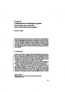
As mentioned earlier, there has been no work reported in the multi-agent systems literature, either centralized or decentralized, on this problem apart from that due to Shehory and Kraus [1998] (henceforth called SK).1 A slightly modified version of this algorithm also appears in [Shehory and Kraus, 1995, 1996]. The algorithm works by making the agents negotiate about which of them performs which of the calculations. In particular, Figure 2.1 details exactly how the algorithm works. Note that the figure only shows the steps that are required for each agent to know its share of calculations (i.e. the figure does not show the steps that are performed to calculate the coalitional values themselves), and that is because we are only interested in the distribution process. Also note that Shehory and Kraus assume that the coalitions are only allowed to contain up to q agents. This is desirable since there could be cases where only coalitions of particular sizes need to be taken into consideration (e.g. if it was known in advance that each of the tasks to be performed requires at least 3 agents, and at most 5 agents, then there 1

In addition to this distribution algorithm, Shehory and Kraus [1998] present an algorithm for coalition structure generation. This algorithm, however, is discussed later in Section 2.2.

18

Chapter 2 Literature Review

19

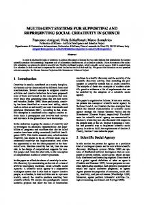
would be no need to consider any of the possible coalitions of sizes {1, 2, 6, 7, . . . , n}). Figure 2.2 shows an example of how the algorithm works given 5 agents.

1: Each agent ai should perform the following: 2:

• Put in Siq every potential coalition that includes up to q agents including ai .

3:

• While Siq is not empty do:

4:

– Contact an agent aj that is a member of a potential coalition in Siq .

5:

– Commit to the calculation of the values of a subset Sijq of the common potential coalitions (i.e. a subset of the coalitions in Siq in which ai and aj are members).

6:

– Subtract Sijq from Siq . Add Sijq to your long-term commitment list Pi .

7:

q – For each agent ak that has contacted you, subtract from Siq the set Ski of the potential coalitions it had committed to calculate values for.

8:

– Calculate the values for the coalitions you have committed to (Sijq ).

9:

– Repeat contacting other agents until Siq = ai (i.e., no more agents to contact). F IGURE 2.1: Shehory and Kraus’s distribution algorithm.

The main advantage of this algorithm is that it operates in a decentralized manner. However, the algorithm suffers from the following major limitations: • The algorithm requires many messages to be sent between the agents, most of which are exponentially large. This is because each agent ai contacts the same agents several times,2 and every time an agent (ai ) contacts another (aj ), it has to send an exponentially large list of coalitions, which is Sijq (see step 7 in Figure 2.1). • Although the algorithm guarantees that every value is calculated at least once, it does not guarantee that each value is calculated exactly once. In fact, when calculating the number of values that were redundantly carried out, we found that this number was exponentially large (see Section 3.4 for more details). This is mainly because the agents have very limited information about each others’ commitments. For example, given 5 agents: a1 , a2 , a3 , a4 , a5 , then if a1 contacts The reason behind this is that when ai contacts aj , it commits to a subset of the coalitions in Siq that contain aj , meaning that ai might later contact aj again, and commit to another subset of the common coalitions, and so on. 2


F IGURE 2.2: Example of how Shehory and Kraus’s distribution algorithm works (given 5 agents).

20


21

a2 and commits to calculate the values of some common coalitions, including {a1 , a2 , a3 , a4 }, and at the same time, a3 contacts a4 and commits to calculate the values of some common coalitions, including {a1 , a2 , a3 , a4 }, then the value of {a1 , a2 , a3 , a4 } would have been calculated twice. • The memory requirements grow exponentially with the number of agents involved. This is because each agent ai needs to maintain the set of potential coalitions in which it is a member, which is Siq (see step 2 in Figure 2.1), as well as the lists that are being received from other agents. Note that each agent might receive several lists simultaneously (a worst-case scenario involves receiving messages from every other agent in the system), in which case the agent needs to have sufficient memory space to maintain all of these lists. • The algorithm provides no guarantees on the quality of its distribution. Specifically, given homogeneous agents, the algorithm does not guarantee that the agents’ shares are equal, and given heterogeneous agents (i.e. with different computational speeds), the algorithm does not guarantee that these differences are efficiently reflected in the distribution.

These limitations make the algorithm both inefficient and inapplicable for large numbers of agents. Against this background, Chapter 3 presents a distribution algorithm that avoids all of these limitations, and meets all of the design objectives that were specified earlier in Section 1.2 (a comparison between this and the SK algorithm can be seen in Section 3.4).

2.2

Solving the Coalition Structure Generation Problem

In this section, we provide a classification of the different algorithms that exist for solving the coalition structure generation problem. Specifically, we identify the following classes: • Low complexity algorithms that return an optimal solution. • Fast algorithms that provide no guarantees on their solutions. • Anytime algorithms that return solutions within a bound from the optimal.


22

In the remainder of this section, we discuss both the advantages and the limitations for each of these classes, and provide examples from the existing literature.

2.2.1

Low Complexity Algorithms that return an Optimal Solution

This class of algorithms is designed to return an optimal solution while minimizing the computational complexity. Note that the emphasis, here, is on providing a guarantee on the performance of the algorithm in worst-case scenarios. One might intuitively think of this class as being the most preferable of all classes. After all, what we are usually interested in is to find an optimal solution and minimize the computational complexity, which is exactly what defines this class of algorithms. However, if such algorithms are to be feasibly applicable, then there is an additional requirement that could even be more crucial than the aforementioned ones, and that is to return a solution as quickly as possible. This is mainly because we are dealing, here, with an exponentially growing search space, meaning that the algorithm, given large numbers of agents, might require a significant amount of time before returning a solution. Based on this, the agents might prefer to use an algorithm that returns a “good” solution very quickly, instead of using an algorithm for which the agents have no time to run to completion. In other words, the agents might be willing to make a trade-off between the quality of the solution, and the time required to run the algorithm. Having identified this class, we shall discuss the state of the art algorithms that belong to it. Note that the time required to run these algorithms depends solely on the number of agents involved (i.e. given the same number of agents, and given different coalition values, the algorithm performs exactly the same number of operations, regardless of the differences in the values). Before going into the details of how these algorithms work, we shall first explain the basic method upon which these algorithms are built, namely dynamic programming, and identify the problems that can generally be solved using this method. Dynamic programming is a method for solving problems that exhibit the properties of optimal substructure and overlapping subproblems [Cormen et al., 2001]: • Optimal substructure (also known as the principle of optimality [Bellman, 1957]) means that, in order to solve a problem, we can break it into subproblems, solve them recursively, and then combine the results to solve the original problem.


23

• Overlapping subproblems means that the subproblems are not independent, that is, subproblems share subsubproblems. A dynamic programming algorithm solves every subsubproblem just once and saves its answer in a table, thereby avoiding the work of recomputing the answer every time the subsubproblem is encountered [Cormen et al., 2001]. In our case, the optimization problem is to find the optimal partition of the set of agents A, and the subproblem is to find the optimal partition of a subset of A. In this context, Yeh [1986] developed a dynamic programming algorithm for solving the complete set partitioning problem. A very similar algorithm was later developed by Rothkopf et al. [1995] for solving the winner determination problem in combinatorial auctions. Note that both algorithms can directly be applied to find optimal coalition structures, since the problems they were originally designed to solve are very similar to the CSG problem (see Section 1.1). Also note that both algorithms are very similar in that they use the same techniques, and have the same complexity. Moreover, explaining how one of them works is sufficient to understand how the other one works. Therefore, we shall only discuss one of these algorithms, namely the one developed by Rothkopf et al. (henceforth called DP). We chose this one because it is relatively simpler and easier to implement). The algorithm is detailed in Figure 2.3, and the way it operates is based on the following observation:

.

Observation 1.1. Let CS ∗ be an optimal coalition structure and let C ∗ ∈ CS ∗ . Also, let C ∗ ⊇ C1 ∪ C2 ∪ . . . ∪ Ck such that these coalitions are pairwise disjoint P (i.e. Ci ∩ Cj = φ for all 1 ≤ i < j ≤ k). Then, v(C ∗ ) ≥ ki=1 v(Ci ).

In other words, if a coalition C ∗ belongs to the optimal coalition structure CS ∗ , then dividing C ∗ into smaller coalitions can never result in a better value for CS ∗ . For example, if an optimal partition of the set A = {1, 2, 3, 4, 5, 6, 7, 8, 9} was as follows: {{1, 2}, {3, 4, 5}, {6}, {7, 8, 9}}, then the optimal partition of the set {1, 2, 3, 4, 5} must be {{1, 2}, {3, 4, 5}}, and similarly, the optimal partition of the set {6, 7, 8, 9} must be {{6}, {7, 8, 9}}. This can be proved by contradiction. Suppose that this was not the case, and that another partition of {6, 7, 8, 9}, say {{6, 7}, {8, 9}}, had a greater value. In this case, {{1, 2}, {3, 4, 5}, {6}, {7, 8, 9}} can no longer be an optimal partition of A, because we could replace {6}, {7, 8, 9} with {6, 7}, {8, 9} and get a greater value (i.e. the optimal partition of A would then be {{1, 2}, {3, 4, 5}, {6, 7}, {8, 9}}).


24

Input: v(C) for all C ⊆ A. If no v(C) is specified then v(C) = 0. Output: the optimal coalition structure, CS ∗ . 1. For all i ∈ {1, . . . , n}, set f1 ({ai }) := {ai }, f2 (ai ) := v({ai }) 2. For i := 2 to n, do: For all C ⊆ A such that |C| = i, do: (a) f2 (C) := max{f2 (C\C 0 ) + f2 (C 0 ) : C 0 ⊆ C and 1 ≤ |C 0 | ≤ 1/2 |C|} (b) If f2 (C) ≥ v(C), set f1 (C) := C ∗ where C ∗ maximizes the right hand side of (a) (c) If f2 (C) < v(C), then set f1 (C) := C, and f2 (C) := v(C). 3. Set CS ∗ := {A}. 4. For every C ∈ CS ∗ , do: If f1 (C) 6= C, then: (a) Set CS ∗ := (CS ∗ \{C}) ∪ {f1 (C), S\f1 (C)}. (b) Goto 4 and start with new CS ∗ . F IGURE 2.3: The DP algorithm for coalition structure generation.

The algorithm requires maintaining two tables in memory, namely f1 and f2 , each having an entry for every possible coalition. Specifically, given a coalition C ⊆ A, f1 (C) would be the optimal partition of C, and f2 (C) would be the value of that partition.3 Note that f1 and f2 are initially not known, and the algorithm gradually computes them as it scans the input, starting from the coalitions of size 2, then 3, then 4, and so on. To better understand how the algorithm works, let us consider the following example, where A = {1, 2, 3, 4} (see Figure 2.4). At first, the algorithm goes through the coalitions of size 2, and for each of these, determines whether to split the coalition in two, or keep it as it is. For example, given C = {1, 2}, the algorithm determines whether {1, 2} is more beneficial than {{1}, {2}}, and that is by comparing the values: v({1, 2}) and v({1}) + v({2}). Both the solution and its value are kept in f1 (C) and f2 (C) respectively.4 The algorithm then moves to the coalitions of size 3. Here, the algorithm also determines whether to split each of these in two, but the decision is now made based on f2 rather than v. For example, given the coalition {1, 2, 3}, the algorithm compares its value with the following values: f2 ({1}) + f2 ({2, 3}), f2 ({2}) + f2 ({1, 3}), and f2 ({3}) + f2 ({1, 2}). Similarly, the algorithm determines whether to split the coalition of size 4 in two. A partition of a coalition C can be defined as a set of coalitions {C1 , . . . , Ck } such that ∪ki=1 Ci = C, and for all 1 ≤ i < j ≤ k, we have Ci ∩ Cj = φ. 4 Actually, in case it was more beneficial to split the coalition in two, rather than keep it as it is, then only one half of the solution needs to be kept in f1 . This is because, by knowing one half, the other half can easily be retrieved. However, to make the example easier to understand, we ignore this fact. Note that this does not affect the performance analysis. 3


25

F IGURE 2.4: Example of how the DP algorithm performs, given a set of agents A = {1, 2, 3, 4}. Here, the arrows show some of the cases where a solution of a subsubproblem is used to find the solution of a subproblem

Note that, by considering all the possible ways of splitting a coalition C in two, and by using f2 instead of v, the optimal partition of C can be found. This comes from Observation 1.1, which implies that if CS ∗ was an optimal partition of A, then by splitting CS ∗ into two disjoint sets of coalitions, namely CS1∗ = {C1,1 , . . . , C1,k1 } : ∪k1 i=1 Ci = A1 , ∗ k2 ∗ and CS2 = {C2,1 , . . . , C2,k2 } : ∪i=1 Ci = A2 , then CS1 must be an optimal partition of A1 , and CS2∗ must be an optimal partition of A2 . In other words, any optimal partitions (containing more than one coalition) must consist of two optimal partitions of two subproblems. The last stage (step 4 in Figure 2.3) would be to find the optimal coalition structure of A, given that we have finished computing f1 and f2 for every possible coalition. This is done as follows. Suppose that the best way to split A in two was the following: (A1 , A2 ),5 this means that the optimal partition of A can be found by combining the optimal partition of A1 with the optimal partition of A2 . Now, each of these two partitions can be found in a similar way. For example, suppose that the best way to divide A1 in two was as follows: (A1,1 , A1,2 ), this means that the optimal partition of A1 can be found by combining the optimal partition of A1,1 with the optimal partition of A1,2 , and so on. This process is repeated until we find a coalition structure in which f1 for every 5

We would know this by looking at f1 (A1 )) which, in this case, must contain one half of the solution (i.e., either A1 or A2 ).


26

coalition contains the coalition itself. In other words, every coalition is better left as it is, rather than split in two. The saving, at this stage, comes from the fact that solutions of subproblems do not need to be recomputed over and over again. For example, we do not need to evaluate both {{1}, {2, 4}} and {{1}, {2}, {4}}, because we already performed the comparison between {2, 4} and {2}, {4} when calculating the best partition of {2, 4}. Similarly, we do not need to evaluate {{2}, {1, 3, 4}}, {{2}, {1}, {3, 4}}, {{2}, {3}, {1, 4}}, {{2}, {4}, {1, 3}}, {{2}, {1}, {3}, {4}}, because we have already done the comparison between all the underlined parts before. The arrows in Figure 2.4 show some of the cases where the solution of a subsubproblem is used to find the solution of a subproblem. The biggest advantage of this algorithm is that it runs in O(3n ) time [Rothkopf et al., 1995]. This is significantly less than exhaustive enumeration of all coalition structures (which is O(nn )). In more detail, this makes the algorithm polynomial in the size of the input. The reason for this is that the input includes 2n values, and the algorithm runs in: O(3n ) = O(2(log2 3)n ) = O((2n )log2 3 )

(2.1)

time. Thus the complexity is O(y log2 3 ), where y is the number of values in the input. Note that no other algorithm in the literature is guaranteed to find the optimal coalition structure in polynomial time (in the size of the input). On the other hand, one of the biggest limitations on using this algorithm is that it cannot generate solutions anytime. This is clearly undesirable, especially given large numbers of agents, because the time required to return the optimal solution might be longer than the time available to the agents. Another limitation on this algorithm (and on dynamic programming in general) is the large number of partial solutions that must be kept in memory. Specifically, the algorithm requires maintaining 3×2n values in memory. This is because for every coalition C, the algorithm requires maintaining v(C), f1 (C), and f2 (C). These limitations make this class of algorithms only suitable for cases where the number of agents is small (e.g. 20 agents or less).


2.2.2

27

Fast Algorithms that provide no Guarantees on their Solutions

These algorithms do not provide any guarantees on finding an optimal solution, nor do they provide worst-case guarantees on the quality of their solutions. Instead, they simply return “good” solutions. However, it is the fact that they can return a solution very quickly, compared to other algorithms, that makes this class of algorithms more applicable, particularly given large numbers of agents. On the other hand, despite the fact that their solutions are usually described as being “good”, one must never forget that these solutions can always be arbitrarily worse than the optimal (i.e. it is not accurate to claim that a solution is “good” just because it was found after a “sufficiently large” subset has been searched; there can always be solutions lying outside this subset that are arbitrarily better than any solution within the subset). In this context, heuristic methods (e.g. simulated annealing, neural networks, and genetic algorithms) provide general ways to search for “good” but not optimal solutions [Skiena, 1998]. Therefore, any algorithm that applies any of these methods can generally be considered to belong to this class of algorithms. Next, we shall discuss two specific examples from the existing literature. In particular, we will first discuss a genetic algorithm that has been developed to solve the CSG problem. After that, we shall discuss another algorithm that applies a different kind of heuristic (i.e. restricting the size of the coalitions taken into consideration). Generally speaking, as long as there is some regularity in the search space (i.e., the evaluation function is not arbitrary), genetic algorithms have the potential to detect that regularity and hence find the coalition structures that perform relatively effectively. To this end, Sen and Dutta [2000] have developed a genetic algorithm for coalition structure generation. The algorithm starts with an initial set of candidate solutions (i.e. a set of coalition structures) called a population, which then gradually evolves toward better solutions. This is done using three main steps: evaluation, selection, and re-combination. In more detail, the algorithm evaluates every member of the current population, selects members based on their evaluation, and constructs new members from the selected ones by exchanging and modifying their contents. More details on the implementation can be found in [Sen and Dutta, 2000]. In addition to being anytime, this algorithm also has additional advantages, compared to the first class of algorithms:


28

• It makes no assumption about how the value of a coalition structure is calculated. In other words, it can be used for CFGs and NFGs. • It scales up well with an increase in the number of agents and hence the size of the search space. As mentioned above, a major limitation on this algorithm (and on genetic algorithms in general) is that the solutions it provides are not guaranteed to be optimal, or even guaranteed to be within a finite bound from the optimal. In other words, these solutions can always be arbitrarily worse than the optimal one. Moreover, even if the algorithm happens to find an optimal solution, one would not be able to verify that this is, indeed, the optimal. This is mainly because genetic algorithms may converge toward a local optima rather than the global optimum of the problem. Another algorithm that belongs to this class of algorithms is the one developed by Shehory and Kraus [1998].6 This algorithm is greedy7 and operates in a decentralized manner. The heuristics they propose (in order to reduce the complexity of finding an optimal coalition structure) involve adding constraints on the size of the coalitions that are allowed to be formed. In more detail, Shehory and Kraus prove that, if only coalition up to a certain size q < n are taken into consideration, then the complexity of the coalition structure generation process can be reduced from exponential to polynomial. Specifically, the algorithm consists of a number of iterative stages. At each stage, the coalition that has the highest value of all permitted coalitions is selected to be formed. The list of permitted coalitions is then updated before another coalition can be selected. The way this is carried out depends on whether the coalitions are allowed to overlap. In more detail, if the coalitions are supposed to be disjoint, then, after a coalition is formed, every other coalition containing members of that coalition are removed from the list. On the other hand, if the coalitions are allowed to overlap, then the coalitions that are removed from the list are only those containing agents that have used all of their resources in previously formed coalitions. Note that the process of selecting the best of all permitted coalitions is carried out in a distributed manner, using the SK algorithm which was discussed earlier in Section 2.1.8 6

Note that this is different from the SK algorithm of Section 2.1 which appeared in the same paper; this algorithm is for coalition structure generation, while the SK algorithm is for distributing value calculations. 7 A greedy algorithm is one that always makes a locally optimal choice in the hope that this choice will lead to a globally optimal solution [Cormen et al., 2001]. 8 However, this process can also be distributed using our DCVC algorithm, and this would, in turn, improve the overall performance of Shehory and kraus’s algorithm for coalition structure generation.


29

Compared to other algorithms, this algorithm has the advantage of being decentralized, as well as being able to take into consideration overlapping coalitions. Moreover, Shehory and Kraus prove that the solution they provide (denoted by CSq0 ) is guaranteed to be within a bound from the optimal solution (denoted by CSq∗ ). However, by optimal, they mean the best possible combination of all permitted coalitions. On the other hand, the algorithm provides no guarantees on the quality of its solutions compared to the ac tual optimal that could be found if all coalitions were taken into consideration. Moreover, although Shehory and Kraus claim that this bound grows logarithmically with the size of the coalitions to which the algorithm refers, we argue that this claim is incorrect. In fact, we can prove that the bound is actually: n/ dn/qe, and that this bound is tight (i.e. no smaller bound can be established). Specifically, given the limit on the size of coalitions to be considered (i.e. q), every coalition structure can include at least dn/qe coalitions, and at most n coalitions. Now, suppose that the solution provided by Shehory and Kraus’s greedy algorithm (i.e. CSq0 ) included dn/qe coalitions, all of which have an equal coalition value v1 = max v(C). In this case, we C have V (CSq0 ) = dn/qe × v1 . Now suppose that all singleton coalitions had a value v2 = v1 − , where is an infinitely small value. In this case, CSq∗ would contain all singleton coalitions, and would have a value V (CSq∗ ) = n × (v1 − ). Based on this, we have: V (CSq∗ )/V (CSq0 ) =

n n × (v1 − ) < dn/qe × v1 dn/qe

As discussed earlier, the main limitation to this class of algorithms is that it provides no guarantees on its solution. However, these algorithms scale up well with the increase in the number of agents, making them particularly suitable for the cases where the number of agents involved is so large that it is impossible to execute any algorithm with exponential complexity.

2.2.3

Anytime Algorithms that return Solutions within a Bound from the Optimal

The reason behind this line of research is that, if the search space was too large to be fully searched, then the other option does not necessarily have to be applying fast algorithms that return “good” solutions with absolutely no worst-case guarantees. Between these two extremes lies a class of anytime algorithms that generate solutions that,


30

although not optimal, are guaranteed to be within a bound from the optimal, and are found by searching pre-defined subsets of the space. These algorithms can improve the quality of their solutions, and establish progressively better bounds, as they search more and more of the search space, until the entire space has been searched, in which case, the bound becomes 1 (i.e. the solution is guaranteed to be optimal). Although these algorithms provide a good balance between execution time and solution quality, they suffer from a major limitation which comes from the fact that no bound can be established on the quality of any solution unless an exponential number of candidate solutions has been examined (this is discussed in more detail later in this section). Next, we discuss a number of algorithm that belong to this class. Sandholm et al. [1999] were the first to introduce an anytime algorithm for coalition structure generation that establishes bounds on the quality of the solution found so far. They view the coalition structure generation process as a search in the coalition structure graph (see Figure 2.5). In this undirected graph, every node represents a possible coalition structure. The nodes are categorized into n levels, where level LVi contains the coalition structures that contain i coalitions. The arcs represent mergers of two coalitions when followed downward, and splits of a coalition into two coalitions when followed upward.

F IGURE 2.5: The coalition structure graph for 4 agents.

Sandholm et al. have proved that, in order to establish a bound on the optimal solution, it is sufficient to search through the first two levels of the coalition structure graph. In


31

The algorithm proceeds as follows: • Search the first two levels of the coalition structure graph. • Continue with a breadth-first search from the bottom of the graph as long as there is time left, or until the entire graph has been searched (this occurs when this breadth-first search completes level 3 of the graph). • Return the coalition structure that has the highest welfare among those seen so far. F IGURE 2.6: Sandholm et al.’s algorithm for coalition structure generation.

this case, the bound would be β = n, and the number of coalition structures searched would be 2n−1 . They have also proved that this bound is tight; meaning that no better bound exists for this search. Moreover, they have proved that no other search algorithm (other than the one that searches the first two levels) can establish any bound while searching only 2n−1 coalition structures or fewer. The main reason for this is that, in order to establish any bound, one needs to go through some subset of coalition structures in which every coalition appears at least once. Otherwise, if a coalition did not appear in any of those structures, and if it happened to be arbitrarily better than every other coalition, then any structure containing it can be arbitrarily better than every structure in the subset. Based on this, the smallest subset of coalition structures that one must search before a bound can be established is the one in which every coalition appears exactly once, and the only subset in which this occurs is the one containing those coalition structures that appear in the first two levels (i.e. those containing one or two coalitions). If the first two levels have been searched, and additional time remains, then it would be desirable to lower the bound with further search. Sandholm et al. have developed an algorithm for this purpose, see Figure 2.6: Sandholm et al. also proved that every time the algorithm finishes searching a particular level, the bound on the optimal can be improved. Specifically, assume that the algorithm has just completed searching level LVi , and let h = b(n − i)/2c + 2, then the bound would be β = dn/he if a ≡ h − 1(modh) and n ≡ i(mod2). Otherwise, the bound would be β = bn/hc. What is interesting here is that, by searching the bottom level (which only contains one coalition structure) the bound drops in half (i.e. β = n/2). Then, to drop β to about n/3, two more levels levels need to be searched. Roughly speaking, the divisor in the


32

bound increases by one every time two more levels are searched, but seeing only one more level helps very little [Sandholm et al., 1999]. Having explained how the algorithm works, we now discuss the advantages and disadvantages of this algorithm. Specifically, this algorithm has the advantage of being anytime, and being able to provide worst case guarantees on the quality of the solution found so far. However, the algorithm has two major limitations: • The algorithm needs to search through the entire search space in order for the bound to become 1. In other words, in order to return a solution that is guaranteed to be optimal, the algorithm simply performs a straight-forward brute-force search. As discussed in Section 1.2, this is intractable even for small numbers of agents. • The bounds provided by the algorithm might be too large for practical use. For example, given 24 agents (i.e. n = 24), and given that the algorithm has finished searching through levels LV1 , LV2 , and LV24 (i.e. after searching through 8,388,609 coalition structures) the bound would be β = n/2 = 12. This means that, in the worst case, the optimal solution can be 12 times better than the current solution. In other words, the value of the current solution is only guaranteed to be no worse than 8.33% of the value of the optimal solution. After that, in order to reduce the bound to β = n/4, four more levels need to be searched, namely LV23 , LV22 , LV21 , and LV20 . This means that by searching through an additional 119,461,563 coalition structures, the value of the solution is guaranteed to be no worse than 16.66% of the optimal value. Similarly, to reduce the bound to β = n/6, the algorithm needs to search through an additional 22,384,498,067,085 coalition structures, and the solution value is then guaranteed to be no worse than 25% of the optimal value. In more detail, Figure 2.7 shows how the bound drops as the number of searched coalition structures increases. As can be seen, it gradually becomes more and more costly to reduce the bound. Moreover, the bound does not go below 2 until every coalition structure has been searched. In other words, if there is just one coalition structure that still needs to be searched, then the value of the solution can only be guaranteed to be no worse than half that of the optimal one. Note that these worst-case guarantees (i.e., 8.33%, 16%, 25%, . . . , 50%) might not be good enough for practical use. Given the limitations of Sandholm et al.’s algorithm, Dang and Jennings [2004] developed an anytime algorithm that can also establish a bound on the quality of the solution


33

F IGURE 2.7: Showing how the bound provided by Sandholm et al.’s algorithm improves with the number of coalition structures examined (given 24 agents).

found so far, but that uses a different search method. Next, we explain how this algorithm works, and then discuss the differences between the two algorithms. To this end, let SL(n, k, c) be the set of all coalition structures that have exactly k coalitions and at least one coalition whose cardinality is not less than c. Also, let SL(n, c) be the set of all coalition structures whose cardinality is between 3 and n − 1 that have at least one coalition whose cardinality is not less than c. That is: SL(n, c) =

n−1 [

SL(n, k, c)

(2.2)

k=3

With these definitions in place, we can express Dang and Jennings’s algorithm (see Figure 2.8). In more detail, the algorithm starts by searching the top two levels, as well as the bottom one (as Sandholm et al.’s algorithm does). After that, however, instead of searching through the remaining levels one by one (as Sandholm et al. do), the algorithm searches through specific subsets of all remaining levels (see Figure 2.9)9 . Specifically, 9

Note that this is not exactly similar to the figure provided in [Dang and Jennings, 2004], in which steps 4, 5, and 6 are shown as subsets that only grow horizontally (i.e. each subset contains solutions from all remaining levels). This is because the figure provided here gives a better understanding of how the search proceeds.


34

The algorithm proceeds as follows: • Search through the sets LV1 , LV2 , LVn • From step 2 onward, search, consequently, through the sets SL(n, dn(d − 1)/de) with d running from b(n + 1)/4c down to 2. That is, search SL(n, dn(bn/4c − 1)/ bn/4ce) at step 2, search SL(n, dn(bn/4c − 2)/(bn/4c − 1)e) at step 3 and so on. Moreover, from step 3 onward, as SL(n, dnd/(d + 1)e) ⊆ SL(n, dn(d − 1)/de) (it is easy to see that SL(n, dn(a − 1)/ae) ⊆ SL(n, dn(b − 1)/be) for every a > b) we only have to search through the set SL(n, dn(d − 1)/de)\SL(n, dnd/(d + 1)e) in order to search through the set SL(n, dn(d − 1)/de). • At each step return the coalition structure with the biggest value (i.e. best social welfare) so far. F IGURE 2.8: Dang and Jennings’s algorithm for coalition structure generation.

the algorithm searches the set of all coalition structures that have k coalitions and at least one coalition structure whose cardinality is not less than dn(d − 1)/de (with d running from b(n + 1)/4c down to 2). Dang and Jennings show that after searching SL(n, dn(d − 1)/de), the algorithm can establish a bound B = 2d − 1.

In general, Dang and Jennings’s algorithm has the same advantages and disadvantages as Sandholm et al.’s. That is, their algorithm is anytime, and provides worst-case guarantees on the quality of the solution found so far, but on the other hand, has to search the entire space in order to verify that the solution found is the optimal one, and the bounds can still be too large for practical use. However, the performance of both algorithms differs in the following ways: • Dang and Jennings claim that their algorithm is faster when smaller bounds are desirable. In more detail, when calculating the number of coalition structures that need to be searched in order to reach a particular bound, the numbers were similar for both algorithms given large bounds. However, as the bounds become smaller, the search required by Dang and Jennings’s algorithm becomes significantly smaller than that required by the other algorithm.10 10

Here, by small, they mean 10 or smaller for the case of 50 agents, and 20 or smaller for the case of 500 agents.


35

F IGURE 2.9: Comparison of the searching path between Dang and Jennings’s and Sandholm et al.’s algorithms.

• The bounds provided by Dang and Jennings’s algorithm are odd integers,11 while the bounds provided by Sandholm et al.’s are not necessarily integral. • While the bound provided by Sandholm et al.’s algorithm does not go below 2 until the whole space has been searched, the bound provided by Dang and Jennings’s algorithm does not go below 3. In other words, since both algorithms will eventually perform a brute-force search, then, during the final stage of performance, Sandholm et al.’s algorithm would have a smaller (i.e. better) bound, compared to Dang and Jennings’s algorithm. To better understand the difference in performance between the two algorithms, we have calculated the amount of search required by each of the algorithms to establish the specified bounds. To this end, Figure 2.10 shows a comparison between the two algorithms 11

This is true except for the initial stage, which goes through levels 1, 2, n. This is because the bound first becomes n (which could be an even integer), and then drops to n/2 (which is not an integer).


36

given 24 agents.12 By looking at the figure, we can see that, as long as the searched portion of the space is smaller than 7.5% of the whole space, the bound provided by Dang and Jennings’s algorithm would be smaller (i.e. better) than that provided by Sandholm et al.’s. However, after 7.5% of the space has been searched, the bound provided by both algorithms becomes very similar, and once 46% of space has been searched, the bound provided by Sandholm et al.’s algorithm drops below 3, while the bound provided by the other algorithms remains at 3 until the whole space has been searched.

F IGURE 2.10: Showing how the bound provided by the two algorithms improves with the number of coalition structures examined (given 24 agents).

Note, however, that both algorithms were not meant for the case where the entire space will eventually be searched. This is because if we had enough time to perform this search, then we would have used the dynamic programming algorithm, which performs this search very quickly. Instead, these algorithms were mainly developed for the cases where the space is too large to be fully searched, even when the dynamic programming algorithm is being used. This means that when evaluating the performance of these algorithms, we are mainly interested in reducing the bound as quickly as possible. In other words, we are mainly interested in the early stages of the performance. Figure 12

We picked the case of 24 agents because it was discussed in the previous subsection. However, when comparing the two algorithms given different numbers of agents, similar results were observed.


37

2.11 is similar to Figure 2.10, except that the number of searched coalition structures is now plotted on a log scale. This makes the figure much more suitable for evaluating the performance of these algorithms, because it gives more weight to the earlier stages of performance. By looking at the figure we can see that, unlike what we have initially expected, both algorithms perform in a broadly similar fashion. However, since the bound provided by Sandholm et al. goes up to 2, as opposed to 3 as per the other algorithm, we consider Sandholm et al.’s algorithm to be the state of the art in this class of algorithms.

F IGURE 2.11: Showing how the bound provided by different algorithms improves with the number of coalition structures examined (given 24 agents). Here, the X values are plotted on a log-scale.

Finally, note that if we only show the amount of search required every time a new bound is established (as in Dang and Jennings [2004]), then we would get the impression that the bound provided by Dang and Jennings is always lower than that provided by the other algorithm (see Figure 2.12). The reason for this confusion is that the number of steps taken by Dang and Jennings’s algorithm is less than that taken by Sandholm et al.’s algorithm, but the reduction in the bound at each step is greater. Therefore, once the bound provided by Dang and Jennings drops, it almost always becomes lower than that provided by the other algorithm. However, since the number of steps is less, the bound remains the same (i.e. the line remains flat) for longer periods, and it is this particular


38

information that is missing from Figure 2.12.

F IGURE 2.12: Showing the number of coalitions structures searched every time a new bound is established (given 24 agents). Here, the X values are plotted on a log scale.

Having discussed two algorithms that use similar techniques, we now discuss a different approach that can also provide solutions anytime, and establish worst-case guarantees on the quality of its solution. This is the linear programming (LP) approach. In the remainder of this subsection, we shall give an overview on LP in general, and specify how it can be applied to solve the CSG problem. Generally speaking, LP problems are optimization problems in which both the objective function and the constraints are linear [Cormen et al., 2001]. Integer programming problems are a special case of linear programming problems in which the decision variables take integer, rather than real, values. The coalition structure generation problem can be formulated as a binary integer programming problem (or a 0-1 integer programming problem), since it only contains binary variables. Specifically, given n agents, the integer model for the CSG problem can be formulated as follows: Maximize

2n P i=1

v(Ci ) × xi


39 subject to Z × X = eT X ∈ {1, 0}n

where Z is an n × 2n matrix of zeros and ones, X is a vector containing 2n binary variables, and eT is the vector of n ones. In more detail, every line in Z represents an agent, and every column represents a possible coalition. As for X, having an element xi = 1 corresponds to coalition Ci being selected in the coalition structure. The first constraint ensures that the selected coalitions are both disjoint and exhaustive. Several techniques have been developed to efficiently solve LP problems (e.g. the dual simplex method, and the interior-point algorithm).13 On the other hand, integer programming problems are much harder to solve. These problems are typically solved by applying linear relaxation coupled with branch-and-bound [Hillier and Lieberman, 2005]. In more detail, the linear relaxation of the problem is obtained simply by deleting (“relaxing”) the integrality constraint, thus ending up with a LP problem (which can be solved quickly using the techniques mentioned earlier). Now if the solution happens to be integral, the problem is solved. Otherwise, two new problems are created by choosing some variable that has a non integer value, and restricting that variable to 1 for one problem, and to 0 for the other. The process is then repeated on each of the new problems. The integer programming approach has an important advantage, which is the fact that it can be applied given any set of coalitions as an input, even if it does not include every possible coalition (i.e., it can applied to both complete and incomplete set partitioning problems). This is particularly useful in cases where only coalitions meeting certain conditions need to be taken into consideration (e.g. if a coalition is only allowed to be formed if it has a certain amount of resources). One the other hand, this approach has a major disadvantage, especially in our case, where the input includes every possible coalition, and that is the huge memory space required to save the search tree. This makes it only applicable for relatively small numbers of agents (see Section 4.3 for more details). After discussing the different approaches to the coalition structure generation problem, we could see that each of these approaches suffers from major limitations, making it either inefficient or inapplicable. This motivates our aim to develop more efficient 13

For more details on these, and other techniques, see [Hillier and Lieberman, 2005].


40

CSG algorithms that can be applied to a wider range of problems, while taking into consideration the objectives outlined in Section 1.2.

2.3

Summary

In this chapter, we have discussed the available algorithm for distributing the coalitional value calculations among cooperative agents (due to Shehory and Kraus), and have shown that it suffers from major limitations, such as performing a large number of redundant operations, requiring significant amounts of communications among the agents, and having infeasibly large memory requirements. These limitations make the SK algorithm inefficient and inapplicable, particularly given large numbers of agents. Against this background, Chapter 3 presents an algorithm that can distribute the coalitional value calculations and, at the same time, avoid all the limitations of the SK algorithm, and meet all of the design objectives placed in Section 1.2 on such a distribution algorithm As for the coalition structure generation problem, we have categorized the available algorithms in the literature into three distinct classes. For each of these classes, we have discussed the main advantages and limitations, and provided examples from existing literature. • As for the first class (i.e. low complexity algorithms that return an optimal solution), we have discussed one example from the literature, namely the dynamic programming algorithm [Yeh, 1986; Rothkopf et al., 1995]. Although this is the only algorithm in the literature that can return an optimal solution in O(3n ) time, the algorithm cannot return solutions anytime, which means that if the agents did not have the time to run the algorithm to completion, then they would end up with no solution at their disposal. Moreover, the algorithm requires building exponentially large tables in memory before it can be executed. • As for the second class (i.e. fast algorithms that provide no guarantees on their solutions), we have discussed two examples from the literature. Specifically, the first example [Sen and Dutta, 2000] uses a genetic algorithm, while the second example [Shehory and Kraus, 1998] sets limitations on the sizes of the coalitions to be considered. Although these algorithms scale up well with the increase in the size of the search space, the solution they provide can always be arbitrarily far from the optimal.


41

• As for the third class (i.e. anytime algorithms that return solutions within a bound from the optimal), we have discussed three examples from the literature. The first example [Sandholm et al., 1999] provides an anytime algorithm that can provide worst-case guarantees on the quality of the solution found so far. As for the second example [Dang and Jennings, 2004], although they claim to outperform Sandholm et al.’s algorithm by orders of magnitude, we have shown that this is not entirely true, and that both algorithms perform in a broadly similar fashion, and have the same advantages and limitations. That is, the algorithms are anytime, and provide a worst-case guarantee on the quality of their solution, but on the other hand, need to search the entire space to return an optimal solution, and provide guarantees that could be too large for practical use. Moving to the third example in the literature (i.e. integer programming), we have shown that this method can be applied to both complete and incomplete set partitioning problems. However, this method requires an infeasibly large memory space, making it only applicable for relatively small numbers of agents. With this in mind, we present in Chapter 4 a novel algorithm for solving the coalition structure generation problem which belongs to the third class of the aforementioned classification. This algorithm can avoid all the limitations that exist in state-of-the-art algorithms belonging to this class, and can meet all of the design objectives placed in Section 1.2 on CSG algorithms.

Chapter 3 Distributing the Coalitional Value Calculations In this chapter, we present our DCVC algorithm for distributing the coalitional value calculations. Here, the agents are assumed to be cooperative (i.e. they carry out their share of computations and they report the results truthfully). However, the underlying algorithm can also be applied in environments where the agents are non-cooperative (i.e. they act to increase their own outcome and may lie about the results if they find it is beneficial to do so). This can be achieved using an additional enforcement mechanism by which the agents are incentivized to calculate all the values they are assigned and to announce the true results they find. However, the exact nature of this mechanism is left for future work at this stage. This chapter is organized as follows. Section 3.1 deals with the case where every agent can join new coalition(s), while Section 3.2 deals with the case where only some of the agents are able/allowed to join new coalitions. The computational complexity of the algorithm is then calculated in Section 3.3, and its performance is evaluated in Section 3.4. Section 3.5 summarizes this chapter.

3.1

The DCVC Algorithm

For illustrative purposes, we start by presenting a basic version of DCVC in which the differences between the agents’ shares are minimized (Section 3.1.1). After that, we show how the required time can be further reduced, by modifying which values an agent calculates, rather than how many values it calculates (Section 3.1.2). Finally, 42

Chapter 3 Distributing the Coalitional Value Calculations

43

we show how DCVC can be modified for the case where the agents have different computation speeds, and prove that the resulting distribution minimizes the computation time (Section 3.1.3). Note that in this section, we assume that every agent is able to join a coalition (Section 3.2 deals with situations where this is not the case).

3.1.1

The Basic Algorithm

In general, the set of possible coalitions can be divided into subsets, each containing the coalitions of a particular size. In DCVC, the distribution of all possible coalitions is carried out by distributing each of these subsets equally among the agents (i.e. agent a1 has x coalitions of size 1 to consider, y of size 2, z of size 3, and so on, and so does a2 , a3 , and so on). This has the following advantages: • An increase in the size of the coalition usually corresponds to an increase in the number of operations required to calculate its value. Therefore, by distributing the coalitions of every size equally among the agents, each agent will not only calculate the same number of values, but also perform the same number of operations. • Any relevant limitations can be placed on the size of the coalitions that can be formed, and this would not affect the distribution quality. The ability to place such limitations is important since the problem under investigation might only require the formation of coalitions of particular sizes (as discussed in Section 2.1). This is also important since it makes DCVC applicable for any coalition formation algorithm that reduces the complexity of the search by limiting the size of the coalitions (as discussed in Section 2.2). Now, let A = {a1 , a2 , . . . , ai , . . . , an } be the set of agents, where n is the number of agents. In order to allow for any limitations on the coalitional sizes, we assume there is a set S of the permitted coalitional sizes. Also, let Ls be an ordered list of possible coalitions of size s ∈ S, and Ns be the number of coalitions in Ls (i.e. Ns = |Ls |). Finally, let Ci,s = {c1i,s , c2i,s , . . . , csi,s } denote the coalition located at index i in the list Ls , where each element cji,s is an integer representing agent acj (For example, Ci,s = i,s {2, 3, 5} corresponds to the coalition of agents a2 , a3 , a5 ). Now, for any s ∈ S, we define the order in the list Ls as follows: • The first coalition in the list is: {n − s + 1, . . . , n}.


44

• The last coalition in the list is: {1, . . . , s}. • Given any coalition Ci,s , the agent can calculate Ci−1,s by checking the values s−2 x x x csi,s , cs−1 i,s , ci,s , . . . until it finds a value ci,s such that ci,s < c1,s , then: – cki−1,s = cki,s : 1 ≤ k < x – cki−1,s = cki,s + 1 : k = x – cki−1,s = ck−1 i−1,s + 1 : x < k ≤ s We assume that the agents know how Ls is ordered, although they do not maintain Ls in memory. An example of the resulting lists is shown in Table 3.1. Here we have n = 6, A = {a1 , a2 , a3 , a4 , a5 , a6 }, S = {1, 2, 3, 4, 5, 6} and N1 , N2 , N3 , N4 , N5 , N6 have the values 6, 15, 20, 15, 6, 1 respectively.

L1 6 5 4 3 2 1

L2 5, 6 4, 6 4, 5 3, 6 3, 5 3, 4 2, 6 2, 5 2, 4 2, 3 1, 6 1, 5 1, 4 1, 3 1, 2

L3 4, 5, 6 3, 5, 6 3, 4, 6 3, 4, 5 2, 5, 6 2, 4, 6 2, 4, 5 2, 3, 6 2, 3, 5 2, 3, 4 1, 5, 6 1, 4, 6 1, 4, 5 1, 3, 6 1, 3, 5 1, 3, 4 1, 2, 6 1, 2, 5 1, 2, 4 1, 2, 3

L4 3, 4, 5, 6 2, 4, 5, 6 2, 3, 5, 6 2, 3, 4, 6 2, 3, 4, 5 1, 4, 5, 6 1, 3, 5, 6 1, 3, 4, 6 1, 3, 4, 5 1, 2, 5, 6 1, 2, 4, 6 1, 2, 4, 5 1, 2, 3, 6 1, 2, 3, 5 1, 2, 3, 4

L5 2, 3, 4, 5, 6 1, 3, 4, 5, 6 1, 2, 4, 5, 6 1, 2, 3, 5, 6 1, 2, 3, 4, 6 1, 2, 3, 4, 5

L6 1, 2, 3, 4, 5, 6

TABLE 3.1: The lists of possible coalitions for 6 agents.

Now, for each agent ai ∈ A, let Ls,i be its share of Ls (i.e. the subset of Ls for which it will calculate values) and Ns,i be the number of coalitions in Ls,i (i.e. Ns,i = |Ls,i |). Given this, we can now express our distribution algorithm (see Figure 3.1). Here, each agent is assumed to know the total number of agents, as well as the set of permitted


45

sizes, we also assume that each agent has a unique global identifier (UID) by which it is identified by other agents. The existence of such an identifier is a reasonable assumption since all agents need to be uniquely identifiable so that messages can be routed correctly.

Each agent ai should perform the following: • Sort the set of agents based on the agents’ UID in an ascending order. • Set: α = 1. • For every s ∈ S, do the following: 1. If (Ns ≥ n) then: 1.1. Calculate the size of your share: Ns,i = bNs /nc 1.2. Calculate the index of the last coalition in your share: indexs,i = i × Ns,i 1.3. Calculate the values of each coalition in your share. 1.4. Calculate the number of additional values that need to be calculated: N 0 = Ns − (n × Ns,i ) Otherwise: 1.5. Calculate the number of additional values that need to be calculated: N 0 = Ns 2. If (N 0 > 0) then: 2.1. Find the sequence of agents A0 in which each agent should calculate one additional value, and if you are a member of A0 , then calculate the appropriate value. This is done as follows: ◦ If (α + N 0 − 1 ≤ n) then: A0 = (aα , aα+1 , . . . , aα+N 0 −1 ) else: A0 = (aα , aα+1 , . . . , an , a1 , . . . , a(α+N 0 −1)−n ) ◦ If (ai ∈ A0 ) then calculate one of the additional values based on your position in A0 ◦ If (α + N 0 ≤ n) then: α = α + N 0 , else: α = α + N 0 − n

F IGURE 3.1: The DCVC algorithm (basic version).

In more detail, each agent starts by sorting the set of agents according to their UID in an ascending order. Note that this is done using a unique key, which means that each agent → will end up with the same sequence, denoted by A. Moreover, the agents implicitly → agree on A without contacting each other; this is because every agent knows that every → other agent also has A. Note that sorting the set of agents is only performed once. For the remainder of this chapter, we will denote by ai the agent located at position i of the → → resulting sequence A. By having an agreement on A, each agent can know which of the → calculations it should perform based on its position in A, this is done as follows. Each agent ai starts by calculating the number of coalitions in Ls,i : Ns,i = bNs /nc

(3.1)


46

The agent then calculates the index in Ls at which Ls,i ends (denoted by indexs,i ). This is done as follows: indexs,i = i × Ns,i

The agent now calculates the values of all the coalitions in Ls,i . This is done without maintaining Ls in memory, or even maintaining Ls,i . Instead, the agent allocates a space of memory, denoted by M = {m1 , . . . , mn }, which is sufficient to maintain one coalition at a time. Basically, the agent starts by setting M to the last coalition in Ls,i (i.e. to the one located at: indexs,i ) and calculates its value. After that, the agent sets M to the coalition before it (i.e. to the coalition located at: indexs,i − 1) and calculates its value, and so on, until the value of every coalition in Ls,i is calculated. Note that the agent so far has calculated the number of coalitions in its share, as well as the index in Ls at which its share ends. This information alone would have been sufficient for the agent to directly know which coalitions belong to its share, but this is only if the agent maintained Ls . However, since this is not the case, then knowing where the coalitions are located in Ls does not imply knowing what those coalitions are. Now from the way the list is ordered, given a coalition in Ls , the agent can always find the coalition before it. Based on this, the agent would only need to set M to the last coalition in Ls,i , and this would be sufficient for it to find all the coalitions in Ls,i . But again, since the agent does not maintain Ls , then knowing the index of the last coalition does not give the coalition directly. For this reason, we show how an agent can find a coalition by only knowing its index in Ls . Generally, the number of all possible coalitions of size s (i.e. the coalitions that contain s agents) out of n agents, is given by the following equation. Here, n! represents n factorial (i.e, if n > 0 then: n! = 1 × 2 × . . . × n, and if n = 0 then n! = 1): Csn =

n! (n − s)! × s!

(3.2)

Now let P (i, {i + 1, . . . , n}) be the list of all possible coalitions of agents ai+1 , . . . , an after adding ai in the beginning of each coalition. Also, let Ps (i, {i + 1, . . . , n}) be the list of all the coalitions in P (i, {i + 1, . . . , n}) that are of size s.1 From 3.2 we find that 1

In other words, Ps (i, {i + 1, . . . , n}) would be the list of all possible coalitions of size (s − 1) that contain agents ai+1 , . . . , an , after adding ai in the beginning of each coalition. By this, each coalition in the list becomes of size s.


47

the number of coalitions in Ps (i, {i + 1, . . . , n}) is: n−i |Ps (i, {i + 1, . . . , n})| = Cs−1

(3.3)

Now, since Ls is ordered as specified earlier, then Ls contains Ps (i, {i + 1, . . . , n}) with i running from n − s + 1 down to 1. For example, for 6 agents, L4 will contain P4 (3, {4, 5, 6}), then P4 (2, {3, 4, 5, 6}) and finally P4 (1, {2, 3, 4, 5, 6}) (see Table 3.1). Therefore, any coalition in Ls that starts with (n − s + 1) − i + 1 must have an index k such that: k>

i−1 X

|Ps ((n − s + 1) − j + 1, {(n − s + 1) − j + 2, . . . , n})|

j=1

k≤

i X

|Ps ((n − s + 1) − j + 1, {(n − s + 1) − j + 2, . . . , n})|

j=1

For example, for 6 agents, any coalition in L4 that starts with 1 must have an index k such that: k > |P4 (3, {4, 5, 6})| + |P4 (2, {3, 4, 5, 6})| = 1 + 4 = 5 k ≤ |P4 (3, {4, 5, 6})| + |P4 (2, {3, 4, 5, 6})| + |P4 (1, {2, 3, 4, 5, 6})| = 1 + 4 + 10 = 15

Therefore, based on 3.3, we know that any coalition in Ls that starts with (n − s + 1) − i + 1 must have an index k such that:

k>

i X

s+j−2 Cs−1

j=1

k≤

i+1 X

s+j−2 Cs−1

j=1

Based on this, we present an algorithm for setting M to the coalition located at indexs,i without maintaining Ls (see Figure 3.2). At first, the agents form what we call a Pascal matrix which is of size: (n − 1) × (n − 1). The matrix includes values from Pascal’s triangle2 and is calculated as follows: 2

More details about Pascal triangles can be found in [Conway and Guy, 1996].


48

1. Set j = 1, index = indexs,i , s1 = s. 2. Check the values: P ascal[s1 , 1], P ascal[s1 , 2], . . . until you find a value: P ascal[s1 , x] ≥ index 3. Set mj = (n − s1 + 1) − x + 1. 4. If (P ascal[s1 , x] = index) then: ◦ Set the rest of the coalition as follows: mk+1 = mk + 1 : k = j, . . . , s − 1 Otherwise: ◦ Set: j = j + 1 , index = index − P ascal[s1 , x − 1] , s1 = s1 − 1 ◦ Move to step 2.

F IGURE 3.2: Setting M to the coalition located at indexs,i in Ls .

P ascal[i, 1] = 1 : ∀i ∈ {1, . . . , n − 1} P ascal[1, j] = j : ∀i ∈ {2, . . . , n − 1} P ascal[i, j] = P ascal[i − 1, j] + P ascal[i, j − 1] : ∀i, j ∈ {2, . . . , n − 1} By this, the following equation holds: P ascal[s, i] =

i X

s+j−2 Cs−1

j=1

Therefore, the agent can find the first member in the required coalition by checking the values: P ascal[s, 1], P ascal[s, 2], . . . until it finds a value P ascal[s, x] such that P ascal[s, x] ≥ indexs,i . The first member would then be (n − s + 1) − x + 1. (Step 1 in Figure 3.3 shows how to find the first member in a coalition that is located at index 46 in the list L5 for 9 agents). Since the first member is (n − s + 1) − x + 1, then the coalition we are looking for must be one of those coalitions that belong to Ls and start with (n − s + 1) − x + 1. Now if we remove the first element from each of these coalitions (since we already know what it is), then we would end up with a new list of coalitions that is similar to Ls−1 . The only difference is that it contains Ps (i, {i + 1, . . . , n}) with i running down to (n − s + 2) − x + 1 instead of running down to 1 (see the list in Figure 3.3, step 2). Note that in this new list, the index of the required coalition becomes: indexs,i − P ascal[s, x − 1] (in our example, the index of the required coalition becomes: 46 − 21 = 25). Based on this, the agent can find the next member in the coalition by checking the values: P ascal[s − 1, 1], P ascal[s − 1, 2], . . . until it finds a value P ascal[s − 1, x] ≥ indexs,i − P ascal[s, x − 1], the next member would then be


F IGURE 3.3: Finding a coalition at index = 46 in the list L5 of coalitions of 9 agents.

49


50

(n − (s − 1) + 1) − x + 1. Similarly, all the members of the coalition can be found. Note that while the agent is checking the values of the Pascal matrix to find some member mj , if it finds a value that is equal to the required index, then the agent can find mj , as well as all the members after it as follows: mk+1 = mk + 1 : k = j, . . . , s − 1. Figure 3.3 shows a complete example for setting M to the coalition at index = 46 in the list L5 for 9 agents. Now that each agent ai has set M to the last coalition in Ls,i , it repeatedly performs the following: • Calculate the value of M .3 • Set M to the coalition before it. This is done by checking the following values: ms , ms−1 , ms−2 , . . . until it finds a value mβ such that mβ < cβ1,s . Then, the values mk : k < β remain unchanged, while the remaining values are calculated as follows: – mk = mk + 1 : k = β – mk = mk−1 + 1 : β < k ≤ s This process should be repeated until all the coalitional values in Ls,i are calculated. Note that after each agent calculates the values in its share, some values might remain uncalculated. This is because Ns might not be exactly divisible by the number of agents, and in this case, the agents’ equal shares will not cover all the required values. In particular, the number of the remaining values would be: 0

N = Ns −

n X

Ns,j = Ns − (n × bNs /nc)

(3.4)

j=1

Here, the coalitions that need their values to be calculated would be: CNs −N 0 +i,s : i ∈ 1, . . . , N 0 . Note that N 0 < n, and that each agent so far has calculated the same number of values. Therefore, in order to calculate these additional values and keep the distribution as fair as possible, each value needs to be calculated by a different agent. In order to do so, the agents need to agree on an ordered set A0 , containing N 0 agents, so that every element of A0 calculates one additional value. In more detail, if we denote by a0i the agent located at index i of A0 , then a0i should calculate the value of coalition CNs −N 0 +i,s . 3

The details of how to calculate a value are left for the developers to decide, based on the problem under investigation (see Section 1.1 for more details).


51

One way of selecting the elements of A0 would be as follows: A0 = {a1 , . . . , aN 0 }. However, since there are more than one list to be distributed, and since each of these lists might contain additional values, then, after the additional values of the current list are calculated, it would be preferable if A0 is updated so that the additional values of the next list, if there are any, are calculated by different agents. This would ensure that the total number of values calculated by each agent will either be equal, or differ by only one value. In order to do so, the agents need to maintain a value α based on which they determine the elements of A0 . Specifically, the value α is initially set to 1, and once the additional values of the current list are calculated, the value α is updated as follows: If (α + N 0 < n) then α = α + N 0 , else α = α + N 0 − n

Using α, the elements A0 can be determined as follows: If (α + N 0 − 1 < n) then A0 = (aα , aα+1 , . . . , aα+N 0 −1 ) else A0 = (aα , aα+1 , . . . , an , a1 , . . . , aα+N 0 −n ) For example, if we have 6 agents, then from equation 3.4 we find that for the list L2 , we have N 0 = 3. Therefore, A0 would be: (a1 , a2 , a3 ) and α becomes 4. Then for L3 , we have N 0 = 2. Therefore, A0 would be (a4 , a5 ) and α becomes 6, and for L4 , we have N 0 = 3. Therefore, A0 would be (a6 , a1 , a2 ) and α becomes 3. Finally, for L6 , we have N 0 = 1, and therefore, A0 would be (a3 ) and α becomes 4 (see A0 in Figure 3.4). After all the values are calculated, the value of α remains 4 instead of being initialized to 1. This means that in order to form other coalitions, any additional calculations will start from a4 . By this, the average number of values calculated by each agent becomes equal.4 To illustrate how DCVC works, Figure 3.4 shows an example of the resulting distribution among 6 agents. As shown in the figure, the agents’ shares are exhaustive and disjoint. Note that this distribution was done without any communication between the agents and without any central decision maker. Moreover, each agent only needed to allocate a space of memory which is sufficient for one coalition. 4

Given a large number of agents, the number of additional values would be insignificant, compared to the total number of values calculated by each agent. However, for a small number of agents, it is worthwhile to add this extra step of updating A0 , rather than simply having A0 = {a1 , . . . , aN 0 }. For example, if we have 6 agents, then by using this extra step, the average number of values calculated by agents: a1 , a2 , a3 , a4 , a5 , a6 would be: 10.5, 10.5, 10.5, 10.5, 10.5, 10.5 respectively, while it would have been: 13, 12, 11, 11, 9, 9, 9 given a fixed A0 .


52

F IGURE 3.4: The resulting distribution for all possible coalitions of 6 agents.

Finally, note that although DCVC gives every agent the ability to save one coalition at a time, the agent can still choose to maintain its entire share of coalitions, provided that it has sufficient memory space. This way, the agent avoids performing the operations required to set M from one coalition to another, throughout the list, every time a coalition is formed.

3.1.2

Modifying the Coalitions to which an Agent is Assigned

By using the distribution process specified earlier, any two agents require an equal time to calculate their share of values. The distribution, however, is done without taking into consideration the time required for each agent to set M from one coalition to another (i.e. the time required to shift M up in the list by 1 coalition). In more detail, after an agent calculates the value of a coalition, it needs to set M to the coalition before it. This is done by performing a number of comparisons and additions as shown earlier in Section 3.1.1. Specifically, changing x values in M requires performing x comparisons, as well as x additions, which gives a total of (2 × x) operations. See Figure 3.5 for an example. As shown in the figure, the agent first searches for β, and then changes the values mβ , mβ+1 , . . . , ms . This means that the agent would perform more operations for smaller values of β. Note that by ordering Ls as specified earlier in Section 3.1.1, β would


53

F IGURE 3.5: Example for setting M to the coalition before it in the list L5 of 9 agents.

generally have smaller values in the coalitions that are located at smaller indices in Ls . → Now since the distribution is done such that the agents located at smaller indices in A calculate the values of the coalitions located at smaller indices in Ls , these agents would generally perform more operations. For example, for the case of 7 agents, Figure 3.6 shows how agents a2 and a6 set M from one coalition to another through the lists L4,2 and L4,6 respectively. As shown in the figure, a2 requires changing a total of 9 values, and thus performs 18 operations, while a6 requires changing a total of 6 values, and thus performs only 12 operations. Therefore, although they both calculate the same number of coalitional values, agent a2 would finish after a6 .

F IGURE 3.6: For the case of 7 agents, the figure shows how a2 and a6 set M from one coalition to another through the lists L4,2 and L4,6 respectively.

The differences between the agents grow with the number of agents involved. For example, for the case of 31 agents, Figure 3.7(A) shows the time required for each agent to set M to the coalitions in its share. As shown in the figure, the required time differs considerably from one agent to another. Now in order to reduce these differences, the


54

distribution needs to be modified. This involves modifying which values an agent calculates, rather than how many values it calculates. In more detail, instead of having agent ai calculate a list of sequential coalitions, ai ’s share can be divided into two sub-lists L1s,i and L2s,i , where each sub-list is located at a different position in Ls . This provides the ability to reduce the differences between the agents by adjusting both the size and the position of the sub-lists of every agent.

F IGURE 3.7: For the case of 31 agents with equal computational speeds, the figure shows the time required for each agent to set M to the coalitions in its share. (A) shows the case where each agent’s share consists of a set of sequential coalitions, while (B) shows the case where each agent’s share is divided into two sub-lists. j j To this end, let Ns,i be the number of coalitions in Ljs,i (i.e. Ns,i = |Ljs,i |), and let indexjs,i be the index in Ls at which Ljs,i ends. The modification can then be expressed as follows:


55

• Each agent ai calculates Ns,i using equation 3.1, and then calculates the number of coalitions in the sub-lists L1s,i and L2s,i as follows:5 1 Ns,i = bNs,i × 0.4c

(3.5)

2 Ns,i = dNs,i × 0.6e

(3.6)

• After that, the agent calculates N 0 using equation 3.4, and then calculates the indices at which the sub-lists end; this is done as follows: 1 index1s,i = i × Ns,i 2 index2s,i = Ns − N 0 − ((i − 1) × Ns,i )

• The calculation of the coalitional values is then handled using the same method specified in Section 3.1.1. In more detail, the modification works as follows. For each agent ai , the sub-list L1s,i is located at the upper part of Ls , and the sub-list L2s,i is located at the lower part. Moreover, the higher L1s,i is, the lower L2s,i is. By this, the total number of operations performed for both sub-lists is broadly the same for all the agents. For example, for the case of 31 agents with equal computational speeds, Figure 3.7(B) shows the modified distribution, as well as the time required for each agent to set M to the coalitions in its share.6 As shown in the figure, the differences between the agents were considerably reduced. In particular, the difference between the first agent to finish and the last dropped from 291 to 17 milliseconds (i.e. it was reduced by 94.2%). Moreover, the time required for the distribution process dropped from 1.236 to 1.081 (i.e. it was reduced by 12.5%). One could argue that the differences between the agents can be further reduced by having more than two sub-lists. However, since setting M to a coalition located at a particular index requires more operations than setting M from one coalition to the next, and since every sub-list requires calculating the index at which it ends, as well as setting M to the coalition located at that index, then, by having more sub-lists, the number of operations required becomes greater, and adjusting both the size and the position of 5

The values 0.4 and 0.6 that are presented in the equations were determined via empirical studies. In this case, a range of different values were explored for a range of coalition scenarios, and these values were consistently the most efficient. 6

The PC on which we ran our simulations had a processor: Pentium(R)4 2.80 GHz, with 1GB of RAM.


56

each sub-list becomes more complicated. Based on this, as well as the fact that having two sub-lists reduces the differences considerably between the agents, we only divide the agents’ shares into two sub-lists.

3.1.3

Considering Different Computational Speeds

As mentioned earlier, the DCVC algorithm distributes the required calculations such that each agent gets an equal share (with a possible difference of at most one calculation). This distribution is efficient if the agents do not need to take into consideration the differences in computational speeds (e.g. because all agents have the same computational speed or because the differences are insignificant). However, in the case where the agents do have significantly different computational speeds, it is inefficient to have each agent calculate the same number of values. In such cases, the distribution needs to be done with respect to the agents’ relative computation speed. In order to do so, we present the required modifications to the algorithm. After sorting the set of agents, and setting α to 1, each agent calculates the time it requires to perform a particular number of operations; the number and type of these operations should be pre-determined by the developers. This can then be used to indicate the agent’s computation speed. For example, the developers can agree on having each agent perform 100000 additions. Then, if agent ai took a time ti = 20 milliseconds, while aj took a time tj = 40, then this indicates that ai has a computational speed twice as fast as aj . Now that each agent ai has calculated ti , it sends this value to every other agent. By this, each agent ai would have tj for every j 6= i. Note that this step is only performed once. The algorithm then distributes the calculations as follows: Instead of calculating the number of coalitions in its share, each agent ai calculates the number of coalitions in every agent’s share. This is done using the following equation: Ns,j =

tj ×

N Pns

k=1

1/tk

1 2 The agent then calculates the values: Ns,i , Ns,i using equations 3.5 and 3.6, and then 1 2 calculates the values: indexs,i , indexs,i using the following equations:


index1s,i =

i X

57

1 Ns,j

j=1

index2s,i

0

= Ns − N −

i−1 X

2 Ns,j

j=1

After each agent calculates the values of the coalitions in its share, some values might remain uncalculated. In this case, the number of the remaining coalitions is given as follows: 0

N = Ns −

n X

Ns,j

j=1

The calculation of these values is then handled using the method defined in Section 3.1.1. We now prove that by using the modified algorithm, we minimize the time required for all the values to be calculated. Theorem 3.1 For any size s ∈ S, the distribution specified in the DCVC algorithm minimizes the time required for all the values to be calculated. Proof. Since the agents perform the calculations in parallel, then the time required for all the values to be calculated is equal to the time required for the last agent to finish calculating its share. Therefore, minimizing the required time is equal to minimizing n the value: max(tj × Ns,j ). Now since we need to distribute the calculation of Ns values j=1

among n agents, we can define the space of possible solutions as the space of vectors P → V ⊆ Rn in which for every vector v ∈ V , we have ni=1 vi = Ns . Then, in order to minimize the value: maxnj=1 (tj × Ns,j ), we need to find a vector x ∈ V that satisfies the following condition: →

∀( y ∈ V )(∃i ∈ {1, .., n}) : ti ×yi < ti ×xi ⇒ (∃j ∈ {1, .., n}) : tj ×yj > tj ×xj ≥ ti ×xi (3.7) That is, decreasing some component xi must be at the expense of increasing some other P component xj such that tj × yj > ti × xi . Now since we have ni=1 xi = Ns , then equation 3.7 implies that: t1 × x1 = t2 × x2 = . . . = tn × xn


58

P By solving this equation, we find that xi = Ns /(ti × nj=1 1/tj ). This means that by P making Ns,i = Ns /(ti × nj=1 1/tj ) for every i ∈ {1, . . . , n}, we minimize the overall time of calculations. j k Pn Note that the agent’s actual share is Ns /(ti × j=1 1/tj ) with a possibility of one additional calculation. This difference, however, is very small and is therefore not considered in the proof.

3.2

Generalizing DCVC to deal with Subsets of Agents

So far, we assumed that every agent is able to join any coalition. However, as discussed earlier, there are cases where this assumption does not always hold. Now let A∗ ⊆ A be the set of agents that are currently able to join any coalition, and let n∗ = |A∗ |. ¯∗n¯ ∗ } be the set of agents that are not able to join any ¯∗2 , . . . , a Similarly, let A¯∗ = {¯ a∗1 , a coalition, where n ¯ ∗ = A¯∗ (this means that: A¯∗ = A\A∗ , and n ¯ ∗ = n − n∗ ). Finally, let P denote the set of all potential coalitions that are of any size s ∈ S, and let P ∗ denote the subset of P in which every coalition contains only members of A∗ . Based on this, every time the agents need to form a coalition, they only need to consider the coalitions that belong to P ∗ . Note that A∗ is continuously changing due to the coalitions that are being formed. Also note that any change in A∗ corresponds to a change in P ∗ , and whenever A∗ = A, we have: P ∗ = P . As mentioned earlier, after a particular coalition is formed, the coalitional values might need to be re-calculated before the agents can form another coalition. Now in order to perform this re-calculation process in a distributed manner, the set P ∗ must first be distributed among the agents. This can be done using either of the following methods: • Searching through P . • Repeating the entire distribution process. We will first discuss the first method since this is the way that the SK algorithm handles the problem, and then we will show that simply repeating the distribution process (which DCVC can do, but SK cannot) is faster and more efficient.


3.2.1

59

Searching through P

In this method, the set P is initially distributed among the agents, and each agent ai maintains its share of P (denoted by Pi ). Then, whenever the coalitional values need to be re-calculated, each agent ai searches through Pi , and finds the coalitions that belong to P ∗ . These coalitions would then be the agent’s share of P ∗ for which it calculates the coalitional values. In more detail, based on the memory that is available to the agent, this can be done using one of the following approaches: 1. Each agent maintains its share of P , but does not maintain its share of P ∗ . Therefore, whenever the coalitional values need to be re-calculated, each agent ai has to search through Pi , and find the coalitions that belong to P ∗ (and that is even if P ∗ remains unchanged). Specifically, finding the coalitions that belong to P ∗ is done by finding those that contain only members of A∗ . Note that we assume every coalition to be written in memory using n bits, where each bit indicates whether an agent is a member of the coalition.7 Therefore, finding whether a coalition belongs to P ∗ is done by first checking the bit that represents a ¯∗1 , and if it is set to 1, then the coalition contains a member of A¯∗ , and therefore does not belong to P ∗ . On the other hand, if it is set to 0, then the agent must check the bit that represents a ¯∗2 , and so on. This is repeated until a member of A¯∗ is found in the coalition, or until all the members of A¯∗ are checked.

2. Each agent ai does not only maintain Pi , but also maintains its share of P ∗ in a temporary list (denoted by tempi ). Obviously, this approach requires allocating a larger memory space (For example, if there are no limitations on the coalitional sizes, then this approach would require allocating 50% more memory space). However, using this approach requires performing fewer operations (see Section 3.3 for details). To show how tempi can be used, let us first consider A¯∗prev to be the previous value of A¯∗ (i.e., A¯∗prev is the set of agents that were not able to join other coalitions during the previous re-calculation process, while A¯∗ is the set of agents that are currently not able to join other coalitions). Also, consider A¯∗removed to be the set of agents that belong to A¯∗prev , but do not belong to A¯∗ , and consider A¯∗added 7

For example, given 8 agents, the coalition {a1 , a2 , a4 , a7 , a8 } can be written in memory as: 11010011 instead of: 1, 2, 4, 7, 8. This way, writing a coalition in memory requires less space, and finding whether an agent belongs to the coalition requires checking a single value instead of searching the entire coalition.


60

to be the set of agents that belong to A¯∗ , but do not belong to A¯∗prev . By this, we have: A¯∗ = (A¯∗prev \ A¯∗removed ) ∪ A¯∗added

: A¯∗removed ∩ A¯∗added = φ

(3.8)

Now, let n ¯ ∗prev be the number of agents in A¯∗prev (i.e., n ¯ ∗prev = A¯∗prev ), and let n ¯ ∗removed , n ¯ ∗added be the number of agents in A¯∗removed and A¯∗added respectively. By this, we have: n ¯∗ = n ¯ ∗prev − n ¯ ∗removed + n ¯ ∗added ∗ Finally, let Pprev be the previous value of P ∗ , let A∗prev be the previous value of A∗ , and let n∗prev = A∗prev . Now, whenever the coalitional values need to be re-calculated, the agents would have one of the following possible cases:

(a) A¯∗removed = φ, and A¯∗added 6= φ (b) A¯∗removed = φ, and A¯∗added = φ (c) A¯∗removed 6= φ, and A¯∗added = φ (d) A¯∗removed 6= φ, and A¯∗added 6= φ Each of these cases needs to be handled differently. Next, for each of these cases, we show how each agent ai can search through Pi to find the coalitions that belong ∗ in tempi ). Here, one should bare to P ∗ (given that it maintains its share of Pprev in mind that, in order to find the coalitions that belong to P ∗ , we need to find the coalitions that do not contain members of A¯∗ . (a) A¯∗removed = φ, and A¯∗added 6= φ : ∗ Here, we have: A¯∗ = A¯∗prev ∪ A¯∗added , and in this case: P ∗ ⊆ Pprev . Thus, ∗ in order to find the coalitions that belong to P , it is sufficient to search ∗ through Pprev (in other words, it is sufficient for each agent ai to search through tempi ) Now since we have: A¯∗ = A¯∗prev ∪ A¯∗added , and since every coalition in tempi does not contain members of A¯∗prev , then in order to know whether a coalition C ∈ tempi contains members of A¯∗ , it is sufficient to know whether it contains members of A¯∗added . Now if it doesn’t, then this coalition belongs to P ∗ . Based on this, each agent ai should search through tempi , and copy the coalitions that do not contain members of A¯∗added to a new list, then free the memory allocated to tempi . This new list would then


61

be the new tempi . (b) A¯∗removed = φ, and A¯∗added = φ : ∗ . Since In this case, we have: A¯∗ = A¯∗prev , which implies that: P ∗ = Pprev ∗ the agents already have their shares of Pprev maintained in memory, then no search is required.

(c) A¯∗removed 6= φ, and A¯∗added = φ : ∗ Here, we have: A¯∗ = A¯∗prev \A¯∗removed , and this implies that: Pprev ⊆ P ∗. In this case, finding the coalitions that belong to P ∗ can be done using two different methods:

• Since tempi contains the coalitions in Pi that do not contain members of A¯∗prev , and since we have: A¯∗prev = A¯∗ ∪ A¯∗removed , then tempi contains the coalitions that do not contain members of A¯∗ and do not contain members of A¯∗removed . Therefore, the agent needs to add to tempi the coalitions that do not contain members of A¯∗ but contain members of A¯∗removed . This is done as follows. For every coalition in Pi , the agent searches for members of A¯∗removed , and if it finds any, then it searches for members of A¯∗ , and if it does not find any, then it adds the coalition to tempi . • This method involves finding the coalitions that belong to P ∗ , without taking into consideration the fact that each agent maintains its share ∗ . In more detail, each agent ai starts by emptying tempi . Afof Pprev ter that, the agent searches through Pi , finds the coalitions that do not contain members of A¯∗ , and copies them to tempi . By using the first method (instead of the second one), any coalition that contains members of A¯∗removed would always require more operations 8 , and any coalition that does not contain members of A¯∗removed might also require more operations.9 Based on this, as well as the fact that the number of coalitions containing members of A¯∗removed is often much larger than those that do not, the agents must then use the second method (i.e. must not take tempi into 8 Because instead of searching for members of A¯∗ , the agent first has to search for members of ∗ ¯ Aremoved , and then search for members of A¯∗ . 9 Because instead of searching for members of A¯∗ , the agent has to search for members of A¯∗removed , and the number of the members of A¯∗removed might be greater than the number of the members of A¯∗ .


62

consideration). (d) A¯∗removed 6= φ, and A¯∗added 6= φ : Here, we have: A¯∗ = (A¯∗prev \A¯∗removed ) ∪ A¯∗added . In this case, finding the coalitions that belong to P ∗ can also be done using two different methods: • Each agent ai should first search through tempi , find the coalitions that do not contain members of A¯∗added , and then copy them to a new list. This new list would then contain the coalitions in Pi that do not contain members of (A¯∗ ∪ A¯∗removed ).10 After that, ai should search through Pi , find the coalitions that do not contain members of A¯∗ , but contain members of A¯∗removed , and then add them to the new list. Finally, ai should free the memory allocated to tempi , and the new list would then be the new tempi . • This method finds the coalitions that belong to P ∗ , without taking into ∗ . consideration the fact that each agent maintains its share of Pprev Here, using the first method (instead of the second one) requires even more operations (compared to the case where: A¯∗removed 6= φ, and A¯∗added = φ). This is because the agent must also search through tempi , and find the coalitions that do not contain members of A¯∗added . Therefore, agent ai performs fewer operations by not taking tempi into consideration.

3.2.2

Repeating the Entire Distribution Process

In this method, the agents simply repeat the entire distribution process of P ∗ whenever A∗ is changed. Note that when using the other distribution algorithm (i.e. the SK algorithm), this method is considered inapplicable, due to the communication that is required every time the distribution process is repeated, as well as the time required to re-build in memory the list containing every coalition in which it is a member. However, when using DCVC, the distribution process can be repeated without any communications between the agents. Moreover, the agents do not have to re-build any lists in memory, thus, reducing the required time (for more details, see Section 3.4). This This is because tempi contains the coalitions in Pi that do not contain members of A∗prev . Then, by finding the coalitions in tempi that do not contain members of A¯∗added , the agent actually finds the coalitions in Pi that do not contain members of A¯∗prev ∪ A¯∗added . And from equation 3.8, we know that (A¯∗prev ∪ A¯∗added ) = (A¯∗ ∪ A¯∗removed ). 10


63

makes repeating the distribution process a feasible possibility. Note that in order to distribute P ∗ (instead of P ), DCVC should be modified as follows: • Replace Ns with Ns∗ in Figure 3.1. This would be sufficient for calculating the number of coalitions in each agent’s share of P ∗ (and not P ), as well as calculating the index of the last coalition in the share, and the number of additional values. • Replace n with n∗ in Figure 3.2. This would be sufficient for setting M to the last coalition in each agent’s share. • Replace n with n∗ when calculating C1,s . By this, C1,s = {n∗ − s + 1, . . . , n∗ − 1, n∗ }. This would be sufficient for setting M to the coalition before it (This is because searching for β is done by comparing values of M with values of C1,s ). Figure 3.8 shows the final version of DCVC, including the modifications mentioned in sections 3.1.2, 3.1.3, and 3.2.2 (henceforth, all references to DCVC refer to this version unless stated otherwise). Here, we assume that the required calculations are distributed among the entire set of agents (A). However, if the distribution is required to be among a subset of A, then two changes need to be made to the algorithm. The first is to replace n with the number of agents that are required to take part in the re-calculation process. The second is to initialize α every time the distribution process is carried out (otherwise, the agents that did not take part in a previous distribution will not be able to know the current value of α).

3.2.3

Comparing the Distribution Efficiency

We will now compare both methods (i.e., searching through P and repeating the entire distribution process) in terms of distribution efficiency (a comparison of both methods, in terms of computational complexity can be seen in Section 3.3): • By having each agent ai search through Pi , the set P ∗ will always be distributed among all of the agents. Note, however, that some agents might have already joined other coalitions, and these agents might be busy performing the tasks they were assigned. Therefore, it might be more efficient if they did not take part in the re-calculation process. Otherwise, if all the agents were always busy performing the search process as well as the value calculation process, then the members


64

of the formed coalitions might not be able to focus on their assigned tasks long enough to actually perform them on time. On the other hand, by repeating the distribution process, the set P ∗ would not necessarily be distributed among all of the agents. Instead, it can be distributed among any subset of A. For example, it can be distributed among those that are not members of any coalition. • When each agent ai searches for the coalitions in Pi that belong to P ∗ , some agents might find significantly more coalitions than others, and thus end up with larger shares of P ∗ . In fact, using this method results in a random distribution of P ∗ . Clearly, this is not optimal since P ∗ needs to be distributed in a way that minimizes the calculation time. On the other hand, repeating the distribution process results in an optimal distribution of P ∗ . Although we have advanced qualitative reasons for the relative advantages of repeating the entire distribution process, we need to provide quantitative results to back this up. To this end, we tested both methods for the case of 30 agents.11 Here, we assume that S = {1, .., 30}, and that the agents have equal computational speeds. Initially, each agent was given an equal share of P . Then, both of the methods were tested given different sizes of A¯∗ (i.e., given different values of n ¯ ∗ , ranging from 0 to 28)12 ; the results were taken as an average of running 50 times, and in every case, the members of A¯∗ were randomly selected from A. Table 3.7 shows the difference between the agent that had the biggest share of the calculations and the one that had the smallest. As shown in the table, by having each agent ai search for the coalitions in Pi that belong to P ∗ , the agents ended up with unequal shares. On the other hand, when repeating the distribution process, the difference between the agents was as small as possible.

3.3

Computational Complexity

As discussed earlier, by repeating the entire distribution process, we obtain an optimal distribution of P ∗ . However, we need to show whether this comes at the expense of an increase in the number of operations required per agent. Therefore, we calculate the computational complexity for each of these methods. Here, we consider the computational complexity to be the number of operations required, given different values of 11

Tests with different numbers of agents were carried out and gave broadly similar results and so they are not shown here. 12 This is because having n ¯ ∗ = 29 means that A∗ contains only one agent, which implies that there is only one potential coalition. In other words, no distribution is required in this case.


65

Each agent ai should first perform the following once: • Sort the set of agents based on the agents’ UID. • Set: α = 1. • If (equal computational speeds = f alse) then: 1. Calculate ti , and send it to every other agent. For every coalition that needs to be formed, each agent ai should perform the following: • For every (s ∈ S, s ≤ n) do the following: 1. If (Ns∗ ≥ n) then: 1.1. If (equal computational speeds): ◦

Calculate the size of your share: Ns,i = bNs∗ /nc

◦

1 2 Calculate the size of both sub-lists: Ns,i = bNs,i × 0.4c , Ns,i = dNs,i × 0.6e

◦

Calculate the number of additional values that need to be calculated: N 0 = Ns∗ − n × Ns,i

1 Calculate the index of the last coalition of each sub-list: index1s,i = i × Ns,i 2 2 ∗ ) indexs,i = Ns −N 0 −((i−1)×Ns,i Otherwise: j k N∗ ◦ Calculate the size of every agent’s share: Ns,j = tj ×Pn s 1/tk : j = 1, . . . , n

◦

k=1

1 Ns,j

2 = bNs,j × 0.4c , Ns,j = dNs,j × 0.6e : j =

◦

Calculate the size of both sub-lists:

◦

Pn Calculate the number of additional values that need to be calculated: N 0 = Ns∗ − j=1 Ns,j Pi 1 Calculate the index of the last coalition of each sub-list: index1s,i = j=1 Ns,j Pi−1 2 0 2 ∗ indexs,i = Ns − N − j=1 Ns,j

1, . . . , n

◦

1.2. Calculate the values of each coalition in your share. Otherwise: 1.3. Calculate the number of additional values that need to be calculated: N 0 = Ns∗ 2. If (N 0 > 0) then: 2.1. Find the sequence of agents A0 in which each agent should calculate one additional value, and if you are a member of A0 , then calculate the appropriate value. This is done as follows: ◦

If (α + N 0 − 1 ≤ n) then: A0 = (aα , aα+1 , . . . , aα+N 0 −1 ) else: A0 = (aα , aα+1 , . . . , an , a1 , . . . , a(α+N 0 −1)−n )

◦

If (ai ∈ A0 ) then calculate one of the additional values based on your position in A0

◦

If (α + N 0 ≤ n) then: α = α + N 0 , else: α = α + N 0 − n

F IGURE 3.8: The DCVC algorithm (final version).

Chapter 3 Distributing the Coalitional Value Calculations n ¯∗ 1 2 3 4 5 6 7 8 9 10 11 12 13 14 15 16 17 18 19 20 21 22 23 24 25 26 27 28

Repeating the distribution 1 1 1 1 1 1 1 1 1 1 1 1 1 1 1 1 1 1 1 1 1 1 1 1 1 1 1 1

66

Searching each agent’s share 4,445,182 5,105,232 3,808,067 1,482,807 1,120,504 679,789 382,358 213,289 116,533 62,869 31,964 16,638 8,290 4,431 2,627 1,402 681 350 197 106 59 29 16 9 4 3 2 1

TABLE 3.2: For the case of 30 agents, the table shows the difference between the agent that had the biggest share of calculations and the one that had the smallest, given different values of n∗ .

n ¯ ∗ . Note that instead of using the big-O notation (which only gives an idea of how the number of operations grows with n ¯ ∗ ), we calculate the complexity using equations that give the exact number of operations required.

3.3.1

Searching through P

Here, each agent ai searches through Pi in order to find the coalitions that belong to the set P ∗ . As mentioned earlier, this can be done using two different approaches:


67

1. If the agents do not maintain their shares of P ∗ , then whenever the coalitional values need to be re-calculated, every agent ai must search through Pi , and find the coalitions that do not contain members of A¯∗ . In this case, the total number of operations is calculated as follows. For every coalition in P , we calculate the number of comparisons required to determine whether it contains members of A¯∗ . In more detail, for every size s ∈ S, we have: • The number of coalitions that require 1 comparison is equivalent to the numn−1 . ber of coalitions in which a ¯∗1 is a member, and that is: Cs−1 • The number of coalitions that require 2 comparisons is equivalent to the number of coalitions in which a ¯∗1 is not a member, and a ¯∗2 is a member, and (n−1)−1 n−2 that is: Cs−1 = Cs−1 . • Similarly, for every i (1 ≤ i < n ¯ ∗ ), the number of coalitions that require i n−i comparisons is given as follows: Cs−1 . • Finally, the number of coalitions that require n ¯ ∗ comparisons is equivalent to the number of coalitions in which a ¯∗1 , . . . , a ¯∗n¯ ∗ −1 are not members, and n−¯ n∗ a ¯∗n¯ ∗ is a member (and that is: Cs−1 ), plus the number of coalitions in which ∗ ∗ ∗ ¯n¯ ∗ are not members (and that is: Csn−¯n ). a ¯1 , . . . , a

Note, however, that there are a number of issues that also need to be considered when calculating the number of comparisons that need to be performed:

• If n ¯ ∗ = 0 (i.e., if all the agents were able to join other coalitions), then we have P = P ∗ , in which case no search is required. • If 0 < n ¯ ∗ < n, then the agents would only need to search through the coalitions that are of size: s ∈ S, s ≤ n − n ¯ ∗ ; this is because A∗ contains only n−¯ n∗ agents (i.e., the agents in A∗ cannot form a coalition that contains more than n − n ¯ ∗ members). • If n ¯ ∗ = n, then no coalition can be formed, and therefore no search is required.


68

Based on this, the number of required operations (denoted by op(¯ n∗ )) is given in the following equation:

op(¯ n∗ ) =

        

P s∈S,s≤n−¯ n∗

0

((

n ¯∗ P

∗

n−i i × Cs−1 ) + (n ¯ ∗ × Csn−¯n ))

if 0 < n ¯∗ < n

i=1

otherwise

Note that the agents search through the coalitions of size: s ≤ n − n ¯ ∗ , and perform a maximum of n ¯ ∗ operations per coalition. Therefore, given a larger value of n ¯ ∗ , the search space would be smaller, but the average number of operations per coalition would be larger. Figure 3.9 shows the total number of operations required, given different values of n ¯ ∗ , and that is for the case of 30 agents.

F IGURE 3.9: The total number of operations required for distributing P ∗ , and that is given 30 agents, where each agent ai searches through Pi without maintaining its share of P ∗ .

As shown in the figure, as long as n ¯ ∗ < 10, the number of operations increases given larger values of n ¯ ∗ . This is because the search space becomes slightly smaller, while the average number of operations required per coalition becomes larger. However, when n ¯ ∗ ≥ 10, the number of operations decreases given larger


69

values of n ¯ ∗ , and that is because the search space becomes significantly smaller.

2. If each agent maintains its share of P ∗ , then whenever the coalitional values need to be re-calculated, the agents would have one of the following possible cases (recall that in order to find the coalitions that belong to P ∗ , we need to find the coalitions that do not contain members of A¯∗ ):

(a) A¯∗removed = φ, and A¯∗added 6= φ : Here, we have: A¯∗ = A¯∗prev ∪ A¯∗added . As mentioned earlier in Section 3.2.1, for every coalition in tempi , agent ai must determine whether it contains members of A¯∗added , and, if not, then the agent must copy it to a new ∗ list. Note that tempi contains the agent’s share of Pprev . Therefore, the total number of operations is calculated as follows. First, for every coali∗ tion in Pprev , we calculate the number of comparisons required to determine whether it contains members of A¯∗added . In more detail, for every size s ∈ S, we have: • The number of coalitions that require 1 comparison is equivalent to the ∗ in which a ¯∗1 is a member, and that is: number of coalitions in Pprev ∗ nprev −1 Cs−1 . • The number of coalitions that require i comparisons, where 1 < i < ∗ n ¯ ∗added , is equivalent to the number of coalitions in Pprev in which a ¯∗1 , . . . , a ¯∗i−1 ∗ n −i prev are not members, and a ¯∗i is a member (and that is: Cs−1 ). • The number of coalitions that require n ¯ ∗added comparisons is equivalent ∗ to the number of coalitions in Pprev in which a ¯∗1 , . . . , a ¯∗n¯ ∗added −1 are not n∗

−¯ n∗

prev added members, and a ¯∗n¯ ∗added is a member (and that is: Cs−1 ), plus the ∗ number of coalitions in Pprev in which a ¯∗1 , . . . , a ¯∗n¯ ∗added are not members

n∗

(and that is: Cs prev

−¯ n∗added

).

Now, we calculate the number of operations required to copy the coalitions ∗ that are in Pprev and do not contain members of A¯∗added . Note that every coalition is maintained in memory using n bits, and that the minimum unit of memory that can be allocated is one byte. Therefore, we can say that every coalition is maintained in an array of dn/8e bytes, and thus, copying a single coalition requires dn/8e operations.


70

Finally, since we have: A¯∗ = A¯∗prev ∪ A¯∗added , and since A¯∗added 6= φ, then: A¯∗ 6= φ, and this implies that n ¯ ∗ > 0. Therefore, n ¯ ∗ can have one of the following values: (1, 2, . . . , n), and for any given value of n ¯ ∗ , the number of required operations is given in the following equation:

op(¯ n∗ ) =

              

if n ¯∗ = n

0


n ¯ ∗added

((

P

n∗

−i

n∗

prev ) + ((¯ n∗added + dn/8e) × Cs prev i × Cs−1

−¯ n∗added

))

i=1

if n ¯∗ < n

Now for the case of 30 agents, Figure 3.10 shows the number of operations required, given different values of n ¯ ∗ . Note that we have: n ¯∗ = n ¯ ∗prev + n ¯ ∗added . Therefore, we calculated op(¯ n∗ ) by taking the average of ¯ ∗ . For example, op(10) was all possible cases, where n ¯ ∗added = 1, 2, . . . , n calculated as an average of the cases where (¯ n∗prev = 9, n ¯ ∗added = 1), and where (¯ n∗prev = 8, n ¯ ∗added = 2), and so on. As shown in the figure, except when n ¯ ∗ < 3, having each agent maintain its share of P ∗ requires fewer operations, especially given large values of n ¯ ∗ . This is because the number ∗ of operations in this case depends mainly on the size of Pprev (which is often much smaller than P ).

(b) A¯∗removed = φ, and A¯∗added = φ : ∗ In this case, we have: P ∗ = Pprev . As mentioned earlier, since the agents ∗ already have their shares of Pprev maintained in memory, then no search is required (i.e. the number of required operations is 0):

op(¯ n∗ ) = 0

(c) A¯∗removed 6= φ, and A¯∗added = φ : As mentioned earlier, finding the coalitions that belong to P ∗ is done without taking into consideration the fact that each agent maintains its share of ∗ Pprev . Instead, each agent ai searches through Pi , and copies the coalitions that do not contain members of A¯∗ to the list tempi . Based on this, the total


71

F IGURE 3.10: Given that A¯∗removed = φ, and A¯∗added 6= φ, the figure shows the total number of operations required to distribute P ∗ , and that is given 30 agents, where each agent maintains its share of P as well as P ∗ .

number of operations is calculated as follows.13 First, for every coalition in P , we calculate the number of comparisons required to determine whether it contains members of A¯∗ . After that, we calculate the number of operations required to copy the coalitions that are in P and do not contain members of A¯∗ . Note that we have A¯∗ = A¯∗prev \A¯∗removed , and A¯∗removed 6= φ. This ¯ ∗ < n. Based on this, n ¯ ∗ can means that n ¯∗ < n ¯ ∗prev , which implies that n have one of the following values: (0, 1, . . . , n − 1), and for any given value, the number of operations is given as follows:

op(¯ n∗ ) =

        


0

((

n ¯∗ P

∗

n−i i × Cs−1 ) + ((¯ n∗ + dn/8e) × Csn−¯n ))

if 0 < n ¯∗

i=1

otherwise

Now for the case of 30 agents, Figure 3.11 shows the number of operations 13

Note that the agent must first empty tempi . However, this is done using a single operation, and, therefore, is not considered when calculating the total number of operations required.


72

required, given different values of n ¯ ∗ . When compared to the case where the agents do not maintain their shares of P ∗ , we find that unless n ¯ ∗ = 0, this method would always require more operations.14 However, as shown in the figure, this difference becomes insignificant when n ¯ ∗ ≥ 8.

F IGURE 3.11: Given that A¯∗removed 6= φ, and A¯∗added = φ, the figure shows the total number of operations required to distribute P ∗ , and that is given 30 agents, where each agent maintains its share of P as well as P ∗ .

(d) A¯∗removed 6= φ, and A¯∗added 6= φ : In this case, finding the coalitions that belong to P ∗ is also done without tak∗ ing into consideration the fact that each agent maintains its share of Pprev . ∗ ∗ ¯ Therefore, op(¯ n ) is calculated just as in the case where Aremoved 6= φ, and ∗ A¯added = φ. Note, however, that we have: (A¯∗ = A¯∗prev \A¯∗removed ∪ A¯∗added : A¯∗removed ∩ A¯∗added 6= φ), and therefore, having: A¯∗added 6= φ, A¯∗removed 6= φ, implies that: 0 < n ¯ ∗ < n. Based on this, the total number of required operations is given as follows: 14

These additional operations would be the ones required to copy the coalitions that do not contain members of A¯∗ .


73

∗

∗

op(¯ n )=

X

n ¯ X ∗ n−i (( i × Cs−1 ) + ((¯ n∗ + dn/8e) × Csn−¯n ))

s∈S,s≤n−¯ n∗

3.3.2

i=1

Repeating the Entire Distribution Process

When repeating the distribution process using DCVC, we distinguish between two different cases, based on the memory that is available to the agent: • In case the agent has sufficient memory space to maintain Pi , then, by maintaining Pi , the agent can avoid repeating the distribution process whenever n ¯ ∗ = 0, because repeating the distribution process in this case would only result in the same share as the one maintained in memory.15 . • In case the memory space is not large enough for agent ai to maintain Pi , then the agent can only repeat the distribution process, even when n ¯ ∗ = 0. Next, we calculate the complexity for the second case (the complexity of the first case can then be calculated easily, by replacing the value with 0 whenever n ¯ ∗ = 0.). Specifically, for every size s ∈ S, we calculate the number of operations required to set M from one coalition to the next, throughout the list.16 As mentioned earlier, changing x values in M requires performing x comparisons, as well as x additions, which gives a total of (2 × x) operations (see Figure 3.5 for an example). Therefore, to calculate the number of operations required, we calculate the number of comparisons, and then multiply this number by 2. In more detail, the number of coalitions that require 1 comparison is equivalent to the number of coalitions in which a∗n∗ is not a member (i.e., ∗ Csn −1 ), and the number of coalitions that require i comparisons, where 1 ≤ i ≤ s, is equivalent to the number of coalitions in which a∗n∗ , . . . , a∗n∗ −(i−1) are not members, n∗ −i and a∗n∗ −i is not a member (i.e, Cs−i+1 ). Based on this, the total number of operations required, in order to set M from one coalition to another, is: ∗

op(¯ n ) = 2×(

X

s X

∗

n −i i × Cs−i+1 )

s∈S, s≤n−¯ n∗ i=1 15

However, the agent in this case might still need to maintain one coalition (instead of maintaining Pi ). This is because the agent, at some point, might need this space to perform other tasks (e.g., the tasks that are assigned to the coalition in which it is a member). 16 Clearly, these are not the only operations required (e.g. operations are also required to calculate the size of each agent’s share, the index at which each share ends, ...etc.). However, we will only consider these when calculating the complexity. This is because we are dealing with an exponential number of coalitions, and, therefore, we only consider the operations that are performed for every coalition. In other words, we only count the operations that grow exponentially with the number of agents.


74

We will now compare the number of operations required, given different values of n ¯∗, and that is when searching through P , and when repeating the distribution process using DCVC. To make this comparison possible, we assume that every agent ai has sufficient memory space to maintain Pi (otherwise, the agents have no other choice but to repeat the distribution process using DCVC). Now, given 30 agents, Figure 3.12 shows the number of operations required to distribute P ∗ using any of the methods that were discussed earlier. Note that when repeating the distribution process (using DCVC), the dashed line shows how the number of operations increases when each agent maintains one coalition (instead of maintaining Pi ). Also note that when searching through P (using tempi ), the figure shows the average number of operations required, and that is for all the different cases of: A¯∗removed , A¯∗added . Unlike what we had initially expected, we found that, on average, repeating the entire distribution process (using DCVC) requires fewer operations, and that is even when the agents do not maintain Pi . Specifically, when compared to the case where each agent searches through Pi (without using tempi ), we find that if each agent maintains Pi , then, repeating the distribution process requires 13.8% of the operations, otherwise, repeating the distribution process requires 27.6% of the operations. Similarly, when compared to the case where each agent searches through Pi (using tempi ), we find that if each agent maintains Pi , then, repeating the distribution process requires 20.3% of the operations, otherwise, it requires 40.7% of the operations.

3.4

Performance Evaluation

Having calculated the computational complexity, we now present empirical results against the SK algorithm. Note that in SK, each agent ai maintains Pi , and whenever the coalitional values need to be re-calculated, the agent finds the coalitions that belong to P ∗ by searching through Pi using tempi (in SK, tempi is equivalent to Lcr i ). As mentioned earlier in Section 3.2, without repeating the entire distribution process, P ∗ would always be distributed among all the agents in A. However, by using SK, every coalition in Pi would be a coalition in which ai is a member, and in this case, P ∗ would


75

F IGURE 3.12: The number of operations required for distributing P ∗ given 30 agents, and that is using different distribution methods.

always be distributed among the members of A∗ instead.17 Note that the agents in A¯∗ might not always be too busy to take part in the re-calculation process. In other words, it would be more efficient if P ∗ can also be distributed among A whenever necessary (as in DCVC). However, since SK only distributes P ∗ among A∗ , then, when comparing the performance of both DCVC and SK, we set DCVC to distribute P ∗ only among A∗ . We tested the performance18 of DCVC and SK given different numbers of agents, ranging from 10 to 25 (However, given any number of agents outside this range, the ratio between the performance of DCVC and SK remains broadly similar). Note that we have 25 agents as a limit, rather than 30 as per the previous sections, because SK requires each agent to maintain a list of all the potential coalitions in which it is a member, and for 30 agents, this list would require more memory space than is actually available to This is because whenever ai ∈ A¯∗ , every coalition in which ai is a member can no longer be formed, including all the coalitions in Pi . In other words, even if ai was able to take part in the re-calculation process, it will not find any coalitions in Pi that belong to P ∗ . 17

18

The PC on which we ran our simulations had a processor: Pentium(R)4 2.80 GHz, with 1GB of RAM.


76

the agent in the simulation. In other words, the agent would not be able to run SK, given N = 30. Given the desiderata mentioned in Section 1.2, we compare the performance of both algorithms based on the following metrics: • Distribution time. • Communication between the agents. • Redundant calculations performed. • Memory requirements. • Equality of the agents’ shares. As for SK, all the results (except the memory requirements) were empirically evaluated rather than theoretically proven. This is because they depend heavily on the order in which the agents contact each other, and there are an exponential number of possible contact sequences, which makes the results non-deterministic and not amenable to a theoretical analysis. As for the time requirements, we deliberately chose empirical evaluation based on clock time; this is because the large memory requirements for SK affect the computer’s performance speed, and this effect will not appear in a theoretical analysis that takes into account only the number of operations performed. As for DCVC, note that when calculating the distribution time, as well as the memory requirements, we distinguish between the case where each agent maintains one coalition, and the case where each agent maintains Pi . This is because the issue of maintaining Pi affects both the distribution time and the memory requirements. In our simulation, the agents initially distribute P among themselves, and after that, given different values of n ¯ ∗ , they distribute P ∗ . The results presented below are for the case where each agent has the same computational speed, and coalitions of any size are allowed to be formed (which means in our terms S = {1, . . . , n}, and in SK’s terms: q = n).19 Section 3.4.1 shows the results for distributing P , while Section 3.4.2 shows the results for distributing P ∗ , given different values of n ¯∗. 19

Note that if there are any limitations on the coalitional sizes, then P would contain a smaller number of coalitions. However, the ratio between the performance of DCVC and SK remains broadly the same.


3.4.1

77

Distributing P

Here, given different numbers of agents (ranging from 10 to 25), we show the results for distributing P among the agents.

3.4.1.1

Distribution Time

The time required to distribute P among the agents is shown in Table 3.3.20 As can be seen, by using DCVC, the agents performed significantly faster, even when each agent maintains its share of P . The reason for this is that when using DCVC, each agent can start processing its share of coalitions immediately, while in SK each agent had to build a list of all the coalitions in which it is a member, and then repeat the process of negotiating with other agents and committing to some coalitions and deleting others, until there are no more agents to contact.

Number of Agents 10 11 12 13 14 15 16 17 18 19 20 21 22 23 24 25

DCVC < 0.01 < 0.01 < 0.01 < 0.01 < 0.01 < 0.01 < 0.01 < 0.01 < 0.01 < 0.01 < 0.01 < 0.01 < 0.01 < 0.01 0.01 0.02

DCVC SK (maintain Pi ) (99% confidence) < 0.01 0.18 ± 1 % < 0.01 1.11 ± 1.2 % < 0.01 1.54 ± 0.9 % < 0.01 0.16 ± 0.5 % < 0.01 1.73 ± 1.4 % < 0.01 1.83 ± 1 % < 0.01 0.36 ± 0.5 % < 0.01 0.32 ± 2.2 % 0.01 0.61 ± 0.3 % 0.02 1.68 ± 2 % 0.04 2.44 ± 1.1 % 0.08 4.81 ± 1.8 % 0.16 10.64 ± 1.9 % 0.33 21.41 ± 4.8 % 0.67 48.99 ± 1.9 % 1.36 108.72± 3.1 %

TABLE 3.3: The time required (in seconds) for the distribution process. 20 Here, we have run the experiments multiple times, and have calculated the standard error of the mean, as well as the 99% confidence intervals. Thus, showing the results in the form: x ± y, means that we are 99% confident that the true mean (i.e. average) lies within the range of values: x − y to x + y. For more details on how to calculate the standard error of the mean, as well as the confidence intervals, see [Altman et al., 2000].

Chapter 3 Distributing the Coalitional Value Calculations 3.4.1.2

78

Communications between the Agents

Table 3.4 shows the total number of bytes that had to be sent between the agents, in order for each one of them to know its share of the calculations. As shown in the table, SK requires sending an exponentially large number of bytes between the agents; this is mainly because if an agent ai contacts another agent aj , and commits to a set of coalitions Sijq , then aj would have to subtract this set from its list, and in order to do so, ai would have to send Sijq to aj . In contrast, DCVC requires no communication between the agents because each of them knows its share by using the provided equations, and not by negotiating with other agents.

Number of agents 10 11 12 13 14 15 16 17 18 19 20 21 22 23 24 25

DCVC 0 0 0 0 0 0 0 0 0 0 0 0 0 0 0 0

SK (99% confidence) 8,799 ± 1 % 20,447 ± 0.8 % 45,076 ± 1.2 % 99,538 ± 0.3 % 217,080 ± 0.5 % 469,173 ± 0.7 % 101,1217 ± 0.7 % 3,242,544 ± 1.5 % 6,888,787 ± 1.6 % 14,644,832 ± 2 % 30,913,264 ± 1.1 % 65,114,817 ± 0.3 % 136,877,925 ± 0.2 % 286,712,976 ± 0.3 % 573,494,824 ± 0.6 % 1,146,989,648 ± 0.2 %

TABLE 3.4: The total number of bytes that had to be sent between the agents.

3.4.1.3

Redundant Calculations Performed

Here by redundant we mean having the value of the same coalition calculated by more than one agent, while it was sufficient for only one agent to calculate it. Table 3.5 shows that using DCVC results in no redundant calculations (because each agent knows the precise bounding of the calculations it should perform, and these are disjoint). In contrast, SK results in an exponentially large number of redundant calculations; this is because each agent’s commitment to a set of coalitions is undertaken with very limited


79

knowledge about the other agent’s commitments. For example, agent ai ’s knowledge q about agent aj ’s commitments is restricted to the set Sji that aj sends to ai . This means that ai is not aware of the coalitions to which aj has committed by contacting other agents. This results in having the agents commit to calculating coalition values without knowing that other agents have already committed to calculating them.

Number of agents 10 11 12 13 14 15 16 17 18 19 20 21 22 23 24 25

DCVC 0 0 0 0 0 0 0 0 0 0 0 0 0 0 0 0

SK (99% confidence) 3,381 ± 1.2 % 8,182 ± 2 % 18,449 ± 3 % 41,584 ± 1.2 % 92,164 ± 4 % 201,827 ± 2.1 % 440,081 ± 1.3 % 949,783 ± 1.2 % 2,034,125 ± 0.1 % 4,357,330 ± 0.3 % 9,255,853 ± 2.4 % 19,607,795 ± 1.7 % 41,431,679 ± 2.1 % 87,182,393 ± 0.9 % 182,993,734 ± 3.5 % 383,229,848 ± 1.2 %

TABLE 3.5: The total number of redundant values that were calculated.

3.4.1.4

Memory Requirements

As mentioned earlier, each coalition is maintained in memory using dn/8e bytes. Given this, Table 3.6 shows the number of bytes required per agent to maintain the necessary coalitions.21 As can be seen, the memory requirements grow exponentially for SK. This is because SK cannot be applied without having each agent start with a list of all the potential coalitions in which it is a member (line 2 in Figure 2.1), and the number of such coalitions is (2n−1 ).22 Note that we did not take into consideration the memory 21 Clearly, this is not the only memory space that is required per agent. For example, one could take into consideration the memory required to save the program that actually performs the algorithm, along with all the variables that are required for this program, such as: n, S, ...etc. However, these do not grow exponentially with the number of agents involved, and thus, are considered insignificant. 22

This is because in the simulation, we assume no limitations P on the coalitional sizes. However, if n−1 there are limitations, then the number of such coalitions becomes: s∈S Cs−1 .


80

space required for the agent to maintain the messages that are received from other agents (which are exponentially large). On the other hand, when using DCVC, each agent only needs to maintain in memory one coalition at a time. This makes DCVC particularly suitable for domains where very little memory space is available for the agents (e.g. agents located on mobile devices).

Number of Agents 10 11 12 13 14 15 16 17 18 19 20 21 22 23 24 25

DCVC 2 2 2 2 2 2 2 3 3 3 3 3 3 3 3 4

DCVC (maintain Pi ) 206 374 684 1,262 2,342 4,370 8,192 23,133 43,692 82,785 157,287 299,595 571,953 1,094,169 2,097,153 5,368,712

SK 1,024 2,048 4,096 8,192 1,6384 32,768 65,536 196,608 393,216 786,432 1,572,864 3,145,728 6,291,456 12,582,912 25,165,824 67,108,864

TABLE 3.6: The minimum number of bytes required per agent to save the necessary coalitions.

As mentioned earlier, given sufficient memory space, each agent using DCVC can also maintain its share of P , and that is to avoid repeating the distribution process whenever P ∗ = P . In this case, the agent would maintain 2n /n coalitions in memory.23 Note that DCVC would still require allocating a smaller memory space, compared to SK, and that is given any number of agents n > 2 (for example, given 25 agents, the memory required by DCVC would only be 8% of that required by SK).

3.4.1.5

Equality of the Agents’ Shares

Since the agents in our simulation are assumed to have equal computational speeds, then the agents’ shares should be as equal as possible. Table 3.7 shows the difference between the agent that had the biggest share of the calculations and the one that had the 23

Given any limitations on the coalitional sizes, this number becomes:

P

s∈S

n−1 Cs−1 /n.


81

smallest. As can be seen, when using DCVC, the maximum difference is only 1, and that is only because the total number of values was not divisible by the given numbers of agents. However with SK, the difference grows exponentially with the number of agents. This is because the agents’ shares are arbitrarily determined based on the order in which they contacted each other. Thus, some agents were contacted by more agents than others, and so removed more coalitions from their list, and ended up with smaller shares. On the other hand, some agents contacted more agents than others, and thus committed to more coalitions, and ended up with larger shares. Number of agents 10 11 12 13 14 15 16 17 18 19 20 21 22 23 24 25

DCVC 1 1 1 1 1 1 1 1 1 1 1 1 1 1 1 1

SK (99% confidence) 51 ± 0.4 % 76 ± 0.4 % 136 ± 0.4 % 215 ± 0.4 % 358 ± 0.5 % 636 ± 0.5 % 962 ± 0.7 % 1,537 ± 1 % 2,882 ± 1.3 % 4,441 ± 1.8 % 7,717 ± 2.8 % 12,094 ± 3.9 % 18,243 ± 6 % 33,568 ± 5.2 % 54,544 ± 5.7 % 85,817 ± 4 %

TABLE 3.7: The difference between the agent that had the biggest share of calculations and the one that had the smallest.

3.4.2

Distributing P ∗

Here, for the case of 25 agents, we show the results for distributing P ∗ , given different values of n ¯∗.

3.4.2.1

Distribution Time

Here, given different values of n ¯ ∗ , Figure 3.12 shows the time required to distribute P ∗ among A∗ . As for DCVC, the dashed line shows how this time increases when each


82

agent maintains one coalition (instead of maintaining Pi ). As for SK, the figure shows the average of all the different cases of: A¯∗removed and A¯∗added . As shown in the figure, using DCVC requires significantly less time, compared to SK. Specifically, by calculating the average for all the different values of n ¯ ∗ , we find that if each agent maintains Pi , then DCVC requires 0.4% of the time, otherwise DCVC requires 0.8% of the time. Note that in Section 3.3, when calculating the number of operations performed, using each of the methods (i.e., repeating the distribution process using DCVC, and searching through P using tempi as in SK), we found that DCVC requires either 20.3% or 40.7% of the operations (depending on whether the agents maintain Pi ). In other words, the difference between both methods was smaller than what we have here. The main reason for this is that when calculating the number of operations required to search through P , we assumed that the agents are searching through exactly |P | coalitions. However, when using SK, the total number of coalitions through which the agents had to search was much larger than |P | (due to the redundancy in the agents’ shares). Another reason for this is that when using SK, the agents were dealing with an exponentially large space of memory (while in DCVC, the agents deal with an extremely small space of memory), and this affects the performance speed. As we mentioned earlier, this effect does not appear when theoretically calculating the number of operations required. Moreover, when using SK, the required operations were not distributed equally among the agents, unlike in DCVC (see Section 3.4.2.5 for details). Note that having unequal shares does not affect the total number of operations performed. However, it does affect the required time. Finally, note that in our simulation, the set P ∗ was distributed among A∗ . However, by using DCVC, the set P ∗ can also be distributed among A whenever applicable. By having more agents taking part in the distribution process, the required time would be even less (for example, given that n = 25 and |A∗ | = 10, distributing P ∗ among all the agents would only take 40% of the time required to distribute it among A∗ ).

3.4.2.2

Communications Between the Agents

Here, note that distributing P ∗ , using either of the two algorithms, is done without any communication between the agents.


83

F IGURE 3.13: For the case of 25 agents, the figure shows the time required to distribute P ∗ among A∗ , given different values of n ¯∗.

3.4.2.3

Redundant Calculations Performed

Table 3.8 shows the total number of redundant values that were calculated, and that is given different values of n ¯ ∗ . As shown in the table, DCVC results in no redundant calculations (because each agent knows the precise bounding of the calculations it should perform, and these are disjoint). In contrast, when using SK, the number of redundant calculations becomes exponentially large (because the agents’ shares of P ∗ are subsets of their shares of P , and these are not disjoint). Note, however, that for smaller values of n ¯ ∗ , the redundancy becomes smaller, since P ∗ becomes smaller.

3.4.2.4

Memory Requirements

Note that by memory requirements, we mean the minimum memory space that must be available to the agent in order for it to perform the distribution algorithm. As for DCVC, distributing P ∗ (instead of P ) does not change the fact that the agent still needs to maintain one coalition at a time (and that the agent might also maintain Pi to avoid repeating the distribution process whenever P ∗ = P ). As for SK, when searching

Chapter 3 Distributing the Coalitional Value Calculations n ¯∗ 0 1 2 3 4 5 6 7 8 9 10 11 12 13 14 15 16 17 18 19 20 21 22 23

DCVC 0 0 0 0 0 0 0 0 0 0 0 0 0 0 0 0 0 0 0 0 0 0 0 0

84

SK (99% confidence) 383,229,848 ± 0 % 183,341,930 ± 0 % 87,514,975 ± 0 % 41,671,477 ± 0 % 19,792,110 ± 0 % 9,374,041 ± 0 % 4,424,080 ± 0 % 2,080,256 ± 0 % 974,435 ± 0 % 454,271 ± 0 % 210,717 ± 0 % 97,156 ± 0 % 44,459 ± 0 % 20,093 ± 0 % 8,987 ± 0.1 % 3,960 ± 0.1 % 1,713 ± 0.2 % 725 ± 0.2 % 297 ± 0.4 % 113 ± 0.6 % 40 ± 1.4 % 13 ± 2.5 % 4 ± 4.8 % 0 ± 11.7 %

TABLE 3.8: For the case of 25 agents, the total number of redundant values that were calculated, given different values of n ¯∗.

for the coalitions that belong to P ∗ , the agent will not be using a memory space that is sufficient to maintain every potential coalition in which it is a member (as when initially distributing P ). However, this does not change the fact that without having this memory space available, the agent will not be able to use SK. Based on this, the memory requirements remain as in Section 3.4.1.4.

3.4.2.5

Equality of the Agents’ Shares

Table 3.9 shows the difference between the agent that had the biggest share of the calculations and the one that had the smallest, and that is given different values of n ¯ ∗ . As can be seen, when using DCVC, the maximum difference is only 1 (and that is only because the total number of values was not divisible by n ¯ ∗ ). On the other hand, when using SK, the difference becomes much larger. This is because when each agent ai searches for the coalitions in Pi that belong to P ∗ , some agents find more coalitions than others, and


85

thus end up with larger shares of P ∗ . Note that for smaller values of n ¯ ∗ , the difference between the agents becomes smaller, because P ∗ becomes smaller. n ¯∗ 0 1 2 3 4 5 6 7 8 9 10 11 12 13 14 15 16 17 18 19 20 21 22 23

DCVC 1 1 1 1 1 1 1 1 1 1 1 1 1 1 1 1 1 1 1 1 1 1 1 1

SK (99% confidence) 85,817 ± 4 % 58,485 ± 5.1 % 35,973 ± 4.8 % 20,738 ± 4.4 % 11,580 ± 4.1 % 6,237 ± 3.5 % 3,301 ± 3 % 1,814 ± 3.2 % 936 ± 3.9 % 498 ± 4 % 259 ± 3.9 % 132 ± 3.8 % 67 ± 4.8 % 45 ± 4.9 % 28 ± 5.7 % 19 ± 6.5 % 13 ± 6.7 % 8±6% 6 ± 6.6 % 5 ± 6.8 % 3 ± 7.4 % 2±9% 1 ± 11.8 % 1 ± 12.7 %

TABLE 3.9: For the case of 25 agents, the table shows the difference between the agent that had the biggest share of the calculations and the one that had the smallest, given different values of n ¯∗.

3.5

Summary

In this chapter, we have presented a basic version of our DCVC algorithm for distributing the coalitional value calculations among cooperative agents. We have shown that the time required to execute DCVC can be reduced by modifying the contents of every agent’s share. We have also shown how DCVC can be modified to reflect any variations in the agents’ computational speeds. After that, we have discussed two different approaches for distributing the value calculations when only a subset of agents can join


86

new coalitions. The first approach involves distributing the whole set of possible coalitions just once, and then having each agent search through its share to find the relevant coalitions that need to be taken into consideration. The second approach is to simply repeat the entire distribution. As we have shown, somewhat surprisingly, the second approach (which DCVC can apply, but SK cannot) is much faster and more efficient. Specifically, it allows the values to be distributed among any set of agents, and guarantees that the distribution is always optimal. We have also presented equations for calculating the exact number of operations required by each of these approaches. Finally, we have benchmarked the performance of DCVC against the SK algorithm, and have shown that our algorithm significantly outperforms it on all relevant dimensions.

Chapter 4 Solving the Coalition Structure Generation Problem In this chapter, we present our Anytime Integer-Partition based Algorithm (AIPA) for coalition structure generation. Specifically, assuming that the value of every coalition is given by a characteristic function v(C) ∈ R+ ∪ {0}, and that the value of every P coalition structure is given by the function V (CS) = C∈CS v(C), our goal is then to search through the set of possible coalition structures (noted as P(A) = {CS ∈ 2A | ∪C∈CS C = A ∧ ∀C, C 0 ∈ CS C ∩ C 0 = ∅}) in order to find an optimal coalition structure (noted as CS ∗ = arg maxCS∈P(A) V (CS)), given v(C), ∀C ⊆ A. This chapter is organized as follows. In Section 4.1, we describe our novel representation for the search space. In Section 4.2, we detail the AIPA algorithm, and show how it can use this representation to prune the search space and find the optimal coalition structure using a branch-and-bound technique. After that, we provide an empirical evaluation of AIPA in Section 4.3. Finally, we summarize the work in Section 4.4.

4.1

Search Space Representation

Recall that the search space representation employed by most existing state-of-theart anytime algorithms is an undirected graph (see Figure 2.5 for an example), where the vertices represent coalition structures [Sandholm et al., 1999; Dang and Jennings, 2004]. This representation, however, forces all valid solutions to be explored in order to guarantee that the optimal has been found. In contrast, the dynamic programming 87

Chapter 4 Solving the Coalition Structure Generation Problem

88

approach (DP) employs a more efficient representation, where solutions of subproblems do not need to be recomputed over and over again [Yeh, 1986; Rothkopf et al., 1995]. This representation, however, does not allow solutions to be generated anytime, which makes it unsuitable when there is insufficient time to wait for an optimal solution. Given the above, we believe an ideal representation for the search space should allow the computation of solutions anytime, while establishing bounds on their quality, and should allow the pruning of the space to speed up the search. With this objective in mind, in this section we describe just such a representation. In particular, it supports an efficient search for the following reasons. First, it partitions the space into smaller independent sub-spaces, for which we can identify upper and lower bounds, and thus, compute a bound on the solutions found during the search. Second, we can prune most of these sub-spaces since we can identify the ones that cannot contain a solution better than the one found so far. Third, since the representation pre-determines the size of coalitions present in each sub-space, agents can balance their preference for certain coalition sizes against the cost of computing the solution for these sub-spaces. Next, we formally define our representation of the search space, and describe its algebraic properties, and, finally, describe worst case bounds on the quality of the solution that our representation allows us to generate.

4.1.1

Partitioning the Search Space

We partition the search space P(A) by defining sub-spaces that contain coalition structures that are similar according to some criterion. The particular criterion we specify here is based on the integer partitions of the number of agents (i.e. n).1 These integer partitions, of an integer n, are the sets of positive integers that add up to exactly n [Skiena, 1998]. For example, the five distinct partitions of the number 4 are {4}, {3, 1}, {2, 2}, {2, 1, 1}, and {1, 1, 1, 1}. It can easily be shown that the different ways in which a set of 4 elements can be partitioned can be directly mapped to the integer partitions of the number 4. For instance, partitions (or coalition structures) of the set of four agents, {{a1 , a2 }, {a3 }, {a4 }} ∈ P(A), and {{a4 , a1 }, {a2 }, {a3 }} ∈ P(A) are associated with the integer partition {2, 1, 1}, where the parts (or elements) of the integer partition correspond to the cardinality of the elements (i.e. the size of the coalitions) of the set partition (i.e. the coalition structure). For example, for the coalition 1

Other criteria could be developed to further partition the space into smaller sub-spaces, but the one we develop here allows us to choose coalition structures with certain properties as we show later.


89

structure {{a4 , a1 }, {a2 }, {a3 }} ∈ P(A), the elements of its configuration can be obtained as follows: |{a4 , a1 }| = 2, |{a2 }| = 1, and |{a3 }| = 1. Note that the number of possible integer partions grows exponentially. However, this number is insignificant compared to the number of possible coalitions or coalition structures. For example, given 24 agents, the number of possible integer partitions is only 1575, while the number of possible coalitions is 16, 777, 215., and the number of possible coalition strucutres is 445, 958, 869, 294, 805, 289. Here, we precisely define this mapping by the function F : P(A) → G, where G is the set of integer partitions of n. Thus, F defines an equivalence relation ∼ on P(A) such that CS ∼ CS 0 iff F (CS) = F (CS 0 ) (i.e. the cardinality of the elements of CS are the same as those of CS 0 ). Given this, for the remainder of this chapter, we will refer to an integer partition as a coalition structure configuration. Then, the pre-image2 of a configuration G, noted as F −1 [{G}], contains all coalition structures with the same configuration G. Figure 4.1 depicts the pre-image F −1 [{G}] as the set of coalition structures corresponding to each configuration G from a set of four agents. We describe the procedure to obtain these pre-images later in this chapter. Note that the levels LVi of the previous representation (i.e. the one used by Sandholm et al. and Dang and Jennings) can easily be obtained as follows: LVi = ∪G∈G,|G|=i F −1 [{G}]. Next, we describe how we can compute bounds for each sub-space F −1 [{G}].

4.1.2

Computing Bounds for Sub-Spaces

For each sub-space F −1 [{G}], it is possible to compute an upper and a lower bound. To this end, we denote by Ls = {C ⊆ A : |C| = s} the list of coalitions of the size s ∈ {1, . . . , n}. Moreover, we denote by maxs , mins , and avgs , the maximum, minimum, and average value of coalitions of a given size s. Now, given a configuQ ration G, we define a set SG = s∈G (Ls )G(s) which is the cartesian product of the coalition lists Ls , where G(s) returns the multiplicity of s in G. For example, given G = {5, 4, 4, 4, 1, 1}, we have SG = (L5 )1 × (L4 )3 × (L1 )2 . Notice that the set SG contains many combinations of coalitions that are considered invalid coalition structures (because they may contain overlapping coalitions). For example, a combination of the following coalitions {a1 , a2 }, {a1 },{a3 } is not a valid coalition structure because agent a1 appears in two coalitions. 2

Recall that the pre-image or inverse image of a set G ⊆ G under F : P(A) → G is the subset of P(A) defined by F −1 [{G}] = {CS ∈ P(A)|F (CS) = G}.


90

F IGURE 4.1: Representing the space using G and F −1 [{G}] and the lists of coalitions Ls . The different levels represent layers used in previous representations where worst case bounds can be established by searching particular layers. The numbers represent the indices of the agents (e.g. 1 for a1 , 4 for a4 ).

Now, consider the value U BG obtained by summing the maximum value of each coaliP tion list involved in a set SG . Formally, U BG = s∈G G(s) · maxs . For example, given G = {5, 4, 4, 1, 1, 1}, we have U BG = max5 + (2 × max4 ) + (3 × max1 ). Now since U BG defines the maximum value of the elements in SG , it is easy to demonstrate that U BG is an upper bound for the maximum value of the coalition structures in F −1 [{G}] (since F −1 [{G}] is a subset of SG ). In a similar way, it is possible to compute a lower P bound. Intuitively, one would expect to select s∈G G(s) · mins (i.e., the minimum value of the elements in SG ) as a lower bound for the maximum value of the coalition structures contained in F −1 [{G}]. However, a better lower bound would be the average of the values of these coalition structures.3 This is because the average value is very likely to be much greater than the minimum one (depending on the distribution of values), and having a greater lower bound allows more pruning of the search space. The key point to note, here, is that the average value of a sub-space can be obtained without having to go through any coalition structure. Instead, we can obtain this average by P summing the averages of the coalition lists (i.e., AV GG = s∈G G(s) · avgs ) and these 3

Generally speaking, an average value can always be considered as a lower bound of the maximum (i.e. optimal) one. This is because the maximum value is at least as good as the average one.


91

can be computed with very little cost by only scanning the input which is much smaller than the space of coalition structures. Theorem 4.1. Let G be a configuration, G = {g1 , . . . , gi , . . . , g|G| }. Let AV GG be the average of all coalition structures in F −1 [{G}] and avggi be the average of all coalitions in Lgi , for every 1 ≤ i ≤ |G|. Then the following holds: AV GG =

X

avggi

gi ∈G

¯ = (g1 , g2 , . . . , gk ) contain the elements of G with a natural ordering Proof. Let G ¯ return all ordered coalition structures (C1,g , . . . , Ck,g ), on them, and let F¯ −1 [{G}] i i Cj,gi ∈ Lgi , where the natural ordering of the elements Cj,gi of each coalition structure ¯ = {1, 1, 2}; is taken into consideration. For example, with n = 4 and G = {1, 1, 2}, G ¯ we have two possibilities: then considering ordered coalition structures in F¯ −1 [{G}], ({a1 }, {a2 }, {a3 , a4 }) and ({a2 }, {a1 }, {a3 , a4 }) that correspond to one coalition structure {{a1 }, {a2 }, {a3 , a4 }} in F −1 [{G}]. Now since the number of repetitions of differ¯ is always the same (e.g., in the above ent coalition structures of F −1 [{G}] in F¯ −1 [{G}] ¯ = {1, 1, 2}, all coalition structures in F −1 [{G}] will appear twice in example with G ¯ F¯ −1 [{G}]), then we have: AV GG = AV GG¯ (4.1) ¯ where AV GG¯ is the average of coalition structures in F¯ −1 [{G}]. Now, if we denote ¯ then we by Nn (g1 , g2 , . . . , gk ) the number of ordered coalition structures in F¯ −1 [{G}], have: AV GG¯ =

1 Nn (g1 , g2 , . . . , gk )

1 = Nn (g1 , g2 , . . . , gk )

X

V (CS)

¯ CS∈F¯ −1 [{G}]

X

k X

v(Ci )

¯ i=1,Ci ∈CS CS∈F¯ −1 [{G}]

Moreover, for every coalition Cj,gi ∈ Lgi , there are: Nn−gi (g1 , g2 , . . . , gi−1 , gi+1 , . . . , gk ) ordered coalition structures where Cj,gi happens to be the j th coalition. Based on this, we have: Nn (g1 , g2 , . . . , gk ) = |Lgi | · Nn−gi (g1 , . . . , gi−1 , gi+1 , . . . , gk )

(4.2)

Moreover, the number of times that v(Cj,gi ) occurs in the j th position of the sum of all ¯ is Nn−g (g1 , . . . , gi−1 , gi+1 , . . . , gk ). Given this, we next coalition values in F −1 [{G}] i


92

compute AV GG¯ as follows:

AV GG¯ =

1 Nn (g1 , g2 , . . . , gk ) k X X Nn−gi (g1 , . . . , gi−1 , gi+1 , . . . , gk ) · v(Cj,gi ) i=1 Cj,gi ∈Lgi

=

k X

X

i=1 Cj,gi ∈Lgi

=

k X

X

i=1 Cj,gi ∈Lgi

=

k X i=1

=

k X



Nn−gi (g1 , . . . , gi−1 , gi+1 , . . . , gk ) · v(Cj,gi ) Nn (g1 , g2 , . . . , gk ) 1 · v(Cj,gi ) (following equation (4.2)) |Lgi |  X · v(Cj,gi )

 1 |Lgi | C

j,gi ∈Lgi

avggi

i=1

As AV GG = AV GG¯ (equation (4.1)), we have: AV GG =

k X

avggi

i=1

4.2

The Anytime Integer-Partition based Algorithm (AIPA)

Having described our representation of the search space, we now describe the main two steps that AIPA requires in order to search the space using this representation: 1. The first step involves obtaining bounds U BG and AV GG for every F −1 [{G}]. While doing so, we can also find the best coalition structures within particular sub-spaces (at a very small cost), and, at the same time, establish a worst-case bound on the quality of the solution found so far, and prune parts of the search space. 2. The second step involves searching within the remaining sub-spaces using a branch-andbound technique to reduce the number of coalition structures that we need to go through, while further pruning the space.


93

Next, we describe each of these steps in more detail.

4.2.1

Step 1: Computing Bounds

The input to the coalition structure generation problem is the value associated to each coalition (i.e. v(C) for all C ∈ 2|A| ). One way of representing this input is to use a table containing every coalition along with its value. Another way of representing it is to agree on an ordering of the coalitions, and to use a list containing only the values of these ordered coalitions (i.e. the first value in the list corresponds to the first coalition, the second value corresponds to the second coalition, and so on). We use the second representation since it does not require maintaining the coalitions themselves in memory. To this end, we assume that the input is partitioned into lists based on the size of the coalitions (i.e. for every size s, we have a list of values Ls corresponding to the coalitions of that size). Moreover, we assume that the coalitions of any given size are ordered both horizontally and vertically (in descending and ascending order respectively) in the list. For example, coalition {a1 , a2 , a4 } has its elements ordered according to their indices and the coalition itself is found above {a1 , a2 , a3 } and below {a1 , a3 , a4 } in the list L3 . This ordering can easily be generated using the techniques applied in DCVC (see Section 3.1.1 for more details). Next, we specify how this input can be scanned. At first, we scan the value of the one coalition of size n (i.e. the grand coalition). This would be the value of the only coalition structure corresponding to G = {n} (i.e. the only coalition structure in LV1 ). After that, we scan the values of the coalitions of size 1 (i.e. singleton coalitions). By summing these values, we get the value of the only coalition structure corresponding to G = {1, 1, . . . , 1} (i.e. the only coalition structure in LVn ). Next, having searched through levels LV1 and LVn , we show how to search through level LV2 at a very low cost during the scanning process. To this end, let G 2 = {G ∈ G : |G| = 2} be the set of configurations where the number of elements in a given G is equal to 2. Then we note that, as a result of the ordering we employ, the two complementary coalitions C and C 0 within any CS ∈ F −1 [{G}], where G ∈ G 2 , are always diametrically positioned in the coalition lists L|C| and L|C 0 | . For example, coalitions {1} and {2, 3, 4} (see Figure 4.1) are diametrically positioned in the list L1 and L3 respectively. Moreover, when |C| = |C 0 |, then the coalitions are diametrically positioned in the same list. For example, coalitions {1, 2} and {3, 4} (see Figure 4.1) can be found at the bottom and top respectively in the list L2 . Given this, we can compute the value of all coalition structures with configurations G ∈ G ∈ by simply summing the values of the coalitions while scanning the lists Ls and Ln−s , starting at different extremities for each list. In so doing, we search through every coalition structure in level LV2 (since we have LV2 = ∪G∈G 2 F −1 [{G}]). Note that we can record maxs and avgs (and maxn−s and avgn−s ) as we are scanning the input. Also note that this process is O(m) where m = 2n − 1 is the size of the input.


94

Having computed maxs and avgs for each sub-space, we can now compute the upper bound (U BG ) and the lower bound (AV GG ) of the maximum value of the elements of every subspace, and that is as described in Section 4.1.2. After that, we can assign the lower bound of the optimal to LB = max(AV G∗G , V (CS 0 )), where AV G∗G = arg maxG∈G (AV GG ) is the highest lower bound of the sub-spaces, and V (CS 0 ) is the value of the best coalition structure CS 0 obtained by scanning the input as above. Hence, all sub-spaces with U BG < LB can be pruned straightaway. For example, as shown in Figure 4.2, sub-spaces corresponding to G = {4}, G = {2, 2}, and G = {1, 1, 1, 1} can be pruned since their upper bounds are less than the lower bound (in this case established by the average of the sub-space corresponding to G = {1, 3}).

F IGURE 4.2: Example of how sub-spaces are pruned based on the bounds calculated. Here, each box represents a sub-space, and the width of each box represents the relative number of coalition structures within the sub-space. After scanning the input, and searching through levels LV1 , LV2 , LVn , we can establish a worstcase bound B =

n 2

on the quality of the solution found so far (according to Sandholm et al.

Chapter 4 Solving the Coalition Structure Generation Problem [1999]). However, we can also specify a worst-case bound equal to

95 U B max AV G∗ 2 ,

where U B max =

G

maxG∈G (U BG ) and AV G∗G 2 = arg maxG∈G 2 (AV GG ). This is because the optimal value is at best equal to U B max , and the best value found so far is at worst equal to the maximum of all average values AV GG of the sub-spaces searched so far (including F −1 [{G}] for all G ∈ G 2 ). Hence, the best (i.e. the smallest) of the two measures can be taken as the worst case bound on the value found so far. Note that

U B max AV G∗ 2

could be much smaller than

G

n 2

(depending on the dis-

tribution of values). In fact, it could be as small as 1 (in which case no further search is required because the best solution found so far is guaranteed to be an optimal one). So far, by only scanning the input, we have calculated maxs and avgs for all s ∈ {1, . . . , n}, we have searched levels LV1 , LV2 , LVn , we have calculated U BG and AV GG for all the sub-spaces within the remaining levels (i.e. LV3 , ..., LVn ), we have pruned some of these sub-spaces, and we have established a worst-case bound on the quality of the solution found so far. Next, we specify how the remaining sub-spaces (if there are any) are searched.

4.2.2

Step 2: Selecting and Searching F −1 [{G}]

Given a set of promising sub-spaces obtained after scanning the input, we need to select the one sub-space F −1 [{G}] to search and then search for the best coalition structure within it ∗ ). These operations are performed repeatedly, one after the other, until either of the (i.e., CSG

following termination conditions are reached, at which point the optimal solution is obtained ∗ ): (i.e., CS ∗ = CSG

∗ ) = U B max (in which case no better coalition structure can exist). 1. V (CSG

2. All nodes have been searched or the remaining sub-spaces have been pruned.

As can be seen, unlike previous CSG algorithms, the speed with which AIPA reaches the optimal value depends on the closeness of the upper bound to the optimal value. This closeness is determined by the spread of the distribution of the coalition values (e.g., a larger variance means that the upper bound is more representative of the maximum and conversely for a tighter variance). Hence, later in this chapter, we will evaluate the robustness of AIPA against a number of distributions. In the next subsection we describe how we select the next sub-space to search.

4.2.2.1

Selecting F −1 [{G}].

To this end, we note that if CS ∗ happens to be located in some sub-space F −1 [{G∗ }], then the only way to find CS ∗ , and to verify that it is indeed an optimal solution, is to search through F −1 [{G∗ }] as well as every other sub-space F −1 [{G}] that has an upper bound U BG ≥ U BG∗ .


96

What would be desirable, then, is to avoid searching through the remaining sub-spaces (i.e. F −1 [{G}] where U BG < U BG∗ ). A key point to note, here, is that, although G∗ is not known in advance, we can still avoid searching through those sub-spaces, and that is by always selecting the next sub-space to search using the following rule: Select F −1 [{G}], where G = arg max(U BG ) G∈G

This selection rule also ensures that, after each sub-space is searched, the upper bound of the optimal (i.e. U B ∗ ) will be reduced (unless if there are several sub-spaces with equal upper bounds). This is illustrated in Figure 4.3. In more detail, the figure shows an example of 10 subspaces (s1 , s2 , ..., s10 ) which are sorted based on their upper bounds, where s1 is the one with the highest upper bound, and s10 is the one with the lowest upper bound. In this example, the optimal solution is located in s3 . This information, however, is not known in advance. Initially, U B ∗ would be equal to the upper bound of s1 , and based on the above rule, the first sub-space to be searched would be s1 . Once s1 is searched, U B ∗ becomes equal to the upper bound of s2 , and once s2 is searched, U B ∗ becomes equal to the upper bound of s3 , and so on. Once s4 is searched, all the remaining sub-spaces (e.g. s5 , ..., s10 ) will be pruned because they have an upper bound lower than the value of the best solution found so far.

F IGURE 4.3: A naive technique for cycling through the coalition structures within F −1 [{G}]. Another reason for using this selection rule is that AIPA only terminates if, either there are no sub-spaces left to be searched or the maximum upper bound has been reached. Either condition can only be reached if the sub-space with the highest U BG (i.e. U B max ) is searched. Note that this rule, which implies best-first search, applies only if we are seeking an optimal solution. In case we are after a near-optimal solution where a bound B ∈ [0, 1] is specified (e.g., B = 0.95 means that the solution sought only needs to be 95% efficient in the worst case), then the selection function will be different since we do not need to search the sub-space with U BG = U B max in order to return a possible solution at any time. Rather, we need to search sub-spaces that are smaller but could give a value close to B × U B max . The point to note is


97

that, given our representation, we can specify B in cases where computing the optimal solution would be too costly and, given this, we can modify the selection function accordingly to speed up the search. Another advantage of being able to control the configuration selected for the search is that agents can choose what type of coalition structures to build according to their computational resources or private preferences [Sandholm et al., 1999; Shehory and Kraus, 1998]. For example, it has been argued that the computation time could be reduced if we could limit the size of the coalitions that could be chosen. However, this is a very costly self-imposed constraint since it possibly means neglecting a number of highly efficient solutions. Instead, by using AIPA, it is possible to determine, ex-ante (before performing the search), which coalition structure configurations are most promising according to their upper and lower bounds. Therefore the computation time can be focused on these configurations and the gains can be traded-off against the computation time since the size of a given sub-space can be exactly computed using the following equation: n−

Pk−2

1 Cgn1 × Cgn−g × . . . × Cgk−1 2 −1 Q |F [{G}]| = n i=1,i∈E(G) G(i)!

i=1

gi

(4.3)

where E(G) is the underlying set4 of elements of G = {g1 , . . . , gk }, and G(i) is the multiplicity of i in G. In cases where agents do prefer coalition structures of particular types (e.g., containing bigger or smaller coalitions), they can now, a priori, balance such preferences with the quality of the solutions (bounded by AV GG ) that can be obtained from such coalition structures. Indeed, this is because, in our case, it is possible to determine the worst-case bound from the optimal that the search of a given subspace will generate (i.e. the elements of the chosen sub-space

4.2.2.2

U Bmax AV GG ).

We next describe how we search

F −1 [{G}].

Searching within F −1 [{G}].

The key point to note, here, is that we are not interested in maintaining a list of every possible coalition structure within the selected F −1 [{G}]. Instead, we are only interested in maintaining the coalition structure that has the maximum value.5 Therefore, we only allocate a space in memory, denoted by M = {M1 , M2 , . . . , M|G| }, which is sufficient to maintain one coalition structure at a time. Then, we use M to cycle through F −1 [{G}] as follows. First, we assign M to one of the coalition structures in F −1 [{G}] and calculate its value. After that, we assign M to another coalition structure in F −1 [{G}] and calculate its value, and so on. This is repeated until every coalition structure in F −1 [{G}] has been examined. While doing so, we record the 4

For example {1, 2} is the underlying set of {1, 1, 2}. This is mainly because maintaining every possible coalition structure requires an infeasibly large memory space (e.g. given 20 agents, one would require 538,600 GB of memory in order to maintain every possible coalition structure). 5


98

coalition structure that has the maximum value found so far. Intuitively, one could perform this cyclation process as shown in Figure 4.4. In more detail, M1 is assigned to one of the coalitions in Lg1 . After that, M2 is used to cycle through Lg2 until a coalition that does not overlap with M1 is found. After that, M3 is used to cycle through Lg3 until a coalition that does not overlap with {M1 , M2 } is found. This is repeated until every Mk ∈ M is assigned to a coalition in Lgk . In this case, M would be a valid coalition structure belonging to F −1 [{G}]. The value of this coalition structure is then calculated and compared with the maximum value found so far. After that, the coalitions in M are updated so as to make M equal to another coalition structure in F −1 [{G}]. Here, we only update Mk once we have examined all the possible instances of {Mk+1 , . . . , , M|G| } that do not overlap with {M1 , . . . , Mk }. For example, in Figure 4.4, we only update M2 (step 5 in the figure) once we have examined all the possible instance of M3 that do not overlap with {M1 , M2 } (steps 2, 3, 4 in the figure). This ensures that M is assigned to different coalition structures, and that, eventually, every possible coalition structures in F −1 [{G}] is examined. Intuitively, one might consider this cyclation technique to be efficient. After all, what we need is to find the coalition structure in F −1 [{G}] that has the maximum value, and this technique guarantees to find such a coalition structure. However, this technique suffers from the following major limitations: • This cyclation technique works by generating combinations of coalitions, and checking whether each of these combinations is a valid coalition structure. In other words, it searches through the space of possible combinations of coalitions. This is a major limitation since the space of coalition structures is already exponentially large, and the last thing we want is to search for it in an even bigger space. For example, given 28 agents, and given G = {1, 2, 3, 4, 5, 6, 7}, the number of coalition structures is only 7.8 × 10−9 of the number of possible combinations. Note that the difference in size between the two spaces grows exponentially with the number of agents involved. Therefore, as long as we are dealing with the space of possible combinations, we will never be able to return solutions in a timely fashion. • Although this technique does not generate the same combination twice, it generates multiple combinations containing the same coalitions, but ordered differently. For example, given n = 7, it could generate the following combinations: {{1, 2}, {3, 4}, {5, 6, 7}} and {{3, 4}, {1, 2}, {5, 6, 7}}). These combinations, however, correspond to the same coalition structure (because the ordering of coalitions within a coalition structure is not taken into consideration). Note that we need to find the coalition structure with the maximum value, and in order to do so, it is sufficient to examine the value of every coalition structure once. In other words, any operation that results in the same coalition structure being generated more than once is considered to be redundant.


F IGURE 4.4: A naive technique for cycling through the coalition structures within F −1 [{G}].

99


100

These limitations are made clearer in the example shown in Figure 4.5. In more detail, given A = {a1 , a2 , a3 , a4 , a5 , a6 , a7 }, and G = {2, 2, 3}, the figure shows that, after assigning M1 to {1, 6}, we had to go through a number of invalid coalitions in L2 before we could find one that does not overlap with M1 . Similarly, after assigning M2 to {2, 3}, we had to go through a number of invalid coalitions in L3 before we could find one that does not overlap with M1 and M2 . The figure also shows an example of different combinations of coalitions corresponding to the same coalitions structure (see the dashed line in the figure).

F IGURE 4.5: Example of how the basic cyclation technique results in a number of invalid combinations being examined, as well as redundant combinations being generated, and that is given A = {a1 , a2 , a3 , a4 , a5 , a6 , a7 } and G = {2, 2, 3}. What would be desirable, then, is to find a way to cycle through the lists Lg1 , . . . , Lg|G| such that only valid combinations are generated. In other words, it would be desirable if Mk only cycles through the valid coalitions in Lgk , rather than going through every coalition in Lgk , and verifying whether it overlaps with {M1 , . . . , Mk−1 }. Moreover, in order to avoid performing any redundant operations, it would be desirable if the cyclation process is guaranteed never to go through the same coalition structure more than once. In what follows, we present a novel cyclation technique that can meet these requirements, and then describe a branch-and-bound approach that avoids generating coalition structures that are known to have a value lower than the maximum one found so far.


101

(1) Avoiding invalid coalition structures: Given G = {g1 , . . . , g|G| }, we define the following sets of agents: A1 , . . . , A|G| , where A1 P contains n agents, and Ak : 2 ≤ k ≤ |G| contains n − k−1 i=1 gi agents. Moreover, we define LCsi as the list of possible combinations of size s taken from the set {1, 2, . . . , i}.6 For example, the list LC23 would contain the following combinations {1, 2}, {1, 3}, and {2, 3}. Given these definitions, we now outline the main differences between our cyclation technique, and the naive one (i.e. the one shown in Figure 4.4): • When using the naive technique, Mk is used to cycle through the list Lgk . On the other |A |

hand, when using our technique, Mk cycles through the list LCgk k . • In the naive technique, having Mk = {Mk,1 , . . . , Mk,gk } implies that Ck = {aMk,1 , . . . , aMk,gk }. On the other hand, when using our technique, it implies that Ck = {Ak,1 , . . . , Ak,gk }. For example, having M2 = {1, 3, 5} does not imply that C2 = {a1 , a3 , a5 }. Instead, it implies that C2 contains the 1st , the 3rd , and the 5th element of A2 . These differences ensure that Mk cycles through all the possible coalitions of size gk taken from Ak .

7

Based on this, if we set Ak to contain the agents that are not members of C1 , . . . , Ck−1 ,

then we ensure that any instance of Ck can never overlap with C1 , . . . , Ck−1 . Figure 4.6 shows an example of our cyclation technique, given A = {a1 , a2 , a3 , a4 , a5 , a6 , a7 } and G = {2, 2, 3}. As can be seen, having M1 = {1, 6} implies that C1 contains the 1st and 6th elements of A1 (i.e. it implies that C1 = {1, 6}). By knowing the agents that belong to C1 , we can then assign A2 to those that do not belong to C1 (i.e. A2 = {2, 3, 4, 5, 7}). As mentioned earlier, M2 would then cycle through all the possible coalitions of size 2 out of A2 , and none of these coalitions would ever overlap with C1 . Similarly, having M2 = {3, 5} implies that C2 contains the 3rd and 5th elements of A2 (i.e. it implies that C2 = {4, 7}), and by knowing the agents that belong to C2 , we can then assign A3 to those that do not belong to C1 or C2 (i.e. |A |

A3 = {2, 3, 5}), and so on. Note that Mk always cycles through the same list (i.e. LCgk k ). |A|

However, every time Ak is updated, the same combination in LCgk would represent a different 6

Note that, throughout this thesis, we use the term “coalition” to represent a combination of agents. Here, however, the elements of the set (i.e. 1, 2, . . . , i) are not used to represent agents (i.e. element i is not used to represent agent ai ). Therefore, we use the term “combination” instead of the term “coalition”. 7

|A |

For example, given A4 = {5, 7, 8} and given g4 = 2, M4 is used to cycle through the list LCg4 4 (i.e. it is used to cycle through LC23 which contains the combinations {1, 2}, {1, 3}, and {2, 3}). In more detail, M4 is first assigned to the combination {1, 2}, and this implies that C4 contains the 1st and 2nd elements of A4 (i.e. it implies that C2 = {5, 7}). After that, M4 is assigned to {1, 3}, and this implies that C4 contains the 1st and 3rd elements of A4 (i.e. it implies that C4 = {5, 8}). Finally, M4 is assigned to {2, 3}, and this implies that C4 contains the 2nd and 3rd elements of A4 (i.e. it implies that C4 = {7, 8}). As can be seen, when M4 finishes cycling through LC23 , all the possible coalitions of size 2 out of A4 (i.e. {5, 7}, {5, 8}, {7, 8}) will be examined.


102 |A|

coalition. Moreover, note that, in order to make Mk cycle efficiently through LCgk , we apply the same procedure that we have developed for our DCVC algorithm (see Section 3.1 for more details).

F IGURE 4.6:

Example of our novel cyclation technique, {a1 , a2 , a3 , a4 , a5 , a6 , a7 } and G = {2, 2, 3}.

given A

=

This cyclation technique ensures that only valid combinations of coalitions (i.e. coalition structures) are generated. Moreover, it ensures that the same combination is never generated twice. However, this cyclation technique can still generate two different combinations containing the same coalitions, but ordered differently. For example, it can still generate the following two valid combinations {{1, 2}, {3, 4}, {5, 6, 7}} and {{3, 4}, {1, 2}, {5, 6, 7}} which correspond to the same coalition structure. As mentioned earlier, this is not desirable because it involves performing redundant operations. Therefore, our cyclation technique needs to be modified so as to guarantee that every coalition structure is only generated once. Next, we show how this can be done. (2) Avoiding redundant coalition structures: We note that, by using our cyclation technique, the same coalition structure can only be generated twice if there are repeated coalition sizes in the configuration (e.g. G = {1, 2, 2, 3} or G = {1, 4, 4, 4, 6}). This is because any coalition structure CS = {C1 , . . . , C|G| } that is generated using our cyclation technique is guaranteed to match the given configuration G. In other words, |Ck | is always equal to gk . Therefore, if a coalition structure CS is generated using our technique, it would be impossible to change the ordering of the coalitions within CS,


103

and still have |Ck | = gk for every 1 ≤ k ≤ |G|, unless if gk = gj where k 6= j. For example, given G = {1, 2, 4}, our cyclation technique can never generate the coalition structure CS = {{1}, {2, 3}, {4, 5, 6, 7, 8}} twice. This is because there is no way to change the ordering of the coalitions within CS, and still have |C1 | = 1, |C2 | = 2, and |C3 | = 5. Based on this, our cyclation technique only needs to be modified whenever we have repeated coalition sizes within G. Note, however, that this is still a serious problem since most of the coalition structures usually contain repeated coalition sizes (e.g. given 20 agents, 99.6% of the possible coalition structures would contain repeated coalition sizes). Here, we assume that the elements within Ak : 1 ≤ k ≤ |G| are listed in an ascending order (see Figure 4.6 where the elements within A1 , A2 , and A3 are ordered ascendingly). Then, assuming that gk = gk+1 , we need to ensure that the same coalitions structure is never generated twice (Figure 4.6 shows an example where g1 = g2 = 2). To this end, note that Mk cycles |A |

through LCgk k starting from the combinations that contain 1, and then moves to those that do not contain 1 but contain 2, and then to those that do not contain 1 or 2 but contain 3, and so on (see Figure 4.6 where the arrow moves from the elements in LC27 that start with 1 to those that start with 2 and so on). Next, we go through each of these cases in detail: |A |

• At first, Mk goes through the combinations in LCgk k that contain 1. For each of these combinations, Ck would contain the 1st element in Ak (i.e. it would contain Ak,1 ). Moreover, for each of these combinations, Mk+1 would go through all the combinations in |A

|

k+1 LCgk+1 . As mentioned earlier, this is done such that Ck+1 never overlaps with Ck . As

a result, Ck+1 would not contain Ak,1 (otherwise it would overlap with Ck ). By the time |A |

Mk finishes cycling through the combinations in LCgk k that contain 1, we would have examined all the coalition structures that contain two coalitions of size gk , where one of them contains Ak,1 , and the other does not. |A |

• After that, Mk moves to the combinations in LCgk k that do not contain 1 but contain 2. For each of these combinations, Ck would not contain Ak,1 , but would contain Ak,2 . Now since we have Ak+1 = Ak \Ck , then Ak,1 would be an element of Ak+1 . In fact, Ak,1 would be the first element in Ak+1 .8 Based on this, whenever Mk+1 cycles through |A

|

k+1 the combinations in LCgk+1 that contain 1, Ck+1 would contain the 1st element in

Ak+1 (i.e. it would contain Ak,1 ). This would, in turn, certainly lead to a repeated coalition structure, because we have already examined all the coalition structures that contain two coalitions of size gk , where one of them contains Ak,1 , and the other does not. To avoid generating these coalition structures twice, we need to make sure that Ck+1 does not contain Ak,1 . This can be done by having Mk+1 cycle through the combinations |A

|

k+1 in LCgk+1 that do not contain 1 (see Figure 4.6 where the combinations in LC27 that

8

This comes from the fact that the elements within Ak are ordered ascendingly (which means that Ak,1 is the smallest element in Ak ), and the fact that Ak+1 is a subset of Ak that contains Ak,1 (which means that Ak,1 is also the smallest element in Ak+1 , and would, therefore, be the first element in it).


104

start with 2 are contained in a box, and this box is only connected to the combinations in LC25 that start with 2, 3, or 4, meaning that whenever M1 cycles through the combinations in LC27 that start with 2, M2 will only cycle through the combinations in LC25 that start |A |

with 2, 3, or 4). By the time Mk finishes cycling through the combinations in LCgk k that contain 2, we would have examined all the coalition structures that contain two coalitions of size gk , where one of them contains Ak,2 , and the other does not. |A |

• Similarly, when Mk moves to the combinations in LCgk k that do not contain 1 or 2 but contain 3, Ck would not contain Ak,1 nor Ak,2 , but would contain Ak,3 . As a result, Ak,1 and Ak,2 would be the first two elements in Ak+1 . Based on this, whenever Mk+1 |A

|

k+1 that contain 1 or 2, Ck+1 would contain the cycles through the combinations in LCgk+1

1st or the 2nd element in Ak+1 respectively (i.e. it would contain Ak,1 or Ak,2 ). This would, in turn, certainly lead to a repeated coalition structure, because we have already examined all the coalition structures that contain two coalitions of size gk , where one of them contains Ak,1 or Ak,1 , and the other does not. In a similar way, this repetition can be |A

|

k+1 avoided by making Mk+1 cycle through the combinations in LCgk+1 that do not contain

1 or 2 (see Figure 4.6 where the combinations in LC27 that start with 3 are contained in a box, and this box is only connected to the combinations in LC25 that start with 3, or 4). |A |

Based on this, whenever Mk cycles through the combinations in LCgk k that start with j, Mk+1 |A

|

k+1 must only cycle through the combinations in LCgk+1 that start with j or higher values. As

|A |

a result, Mk can only cycle through the combinations in LCgk k that start with j such that 1 ≤ j ≤ (|Ak+1 | − gk+1 + 1). Otherwise, if j > (|Ak+1 | − gk+1 + 1), then there would |A

|

k+1 be no combinations in LCgk+1 that start with j or higher values (e.g. in Figure 4.6, we have

(|A2 | − g2 + 1) = (5 − 2 + 1) = 4. Based on this, M1 can only cycle through the combination in LC27 that start with 1, . . . , 4, because there are no combinations in LC25 that start with 5 or 6). Similarly, if we have more than two coalitions of the same size (i.e. if we have |A |

gk = gk+1 = . . . = gk+x ), then Mk can only cycle through the combinations in LCgk k that start with j such that 1 ≤ j ≤ (|Ak+x | − gk+x + 1). These modifications ensure that our cyclation technique generates every possible coalition structures within the selected F −1 [{G}] exactly once. However, it would be even more desirable if we can avoid generating the coalition structures that cannot have a value greater than the maximum value found so far. Next, we show how this can be done using branch-and-bound techniques. (3) Applying Branch-and-Bound: As mentioned earlier, when cycling through the coalition structures within F −1 [{G}], we only update Mk once we have examined all the possible instances of {Ck+1 , . . . , C|G| } that do not overlap with {C1 , . . . , Ck }. In other words, we only update Mk once we have examined


105

all the possible coalition structures that start with {C1 , . . . , Ck }. However, if we knew that none of these coalition structures could have a value greater than the maximum value found so far, then we could update Mk straight away (i.e. without having to go through any of the possible instances of {Ck+1 , . . . , C|G| }). In order to do so, we calculate an upper bound on the value of the coalitions that can be added to {Ck+1 , . . . , C|G| }. Specifically, having computed maxs for every possible coalition size s ∈ {1, 2, . . . , n}, we can then calculate such P|G| an upper bound as follows: U B{gk+1 ,...,g|G| } = i=k+1 maxgi . Now, let LB be the value of Pk the current best solution found so far, and let V (C1 , . . . , Ck ) = i=1 v(Ci ). Then, having LB > V (C1 , . . . , Ck ) + U B{gk+1 ,...,g|G| } implies that none of the coalition structures that start with {C1 , . . . , Ck } and end with coalitions of sizes gk+1 , . . . , g|G| can have a value greater than the best value found so far. On the other hand, having LB ≤ V (C1 , . . . , Ck ) + U B{gk+1 ,...,g|G| } does not necessarily imply that all of these coalition structures need to be examined. This is because, for every coalition Ck+j , we can still have: LB > V (C1 , . . . , Ck+j )+U B{gk+j+1 ,...,g|G| } . Graphically, this is expressed by avoiding the move to the rightmost lists as in Figure 4.7.

F IGURE 4.7: Applying branch-and-bound while searching through the coalition structures within F −1 [{G}].

4.3

Experimental Evaluation

In this section, we empirically evaluate and benchmark the AIPA algorithm. The general hypothesis is that it should perform better than those that have previously been developed for this


106

task. However, a potential criticism that can be leveled against AIPA is that, contrary to the other approaches, it is dependent on computing upper and lower bounds that are relatively close to the actual optimal value in order to prune large parts of the space and so guarantee that the optimal value has been found. Since this closeness to the optimal is determined by the spread of the distribution of the values of the coalitions, it is crucial that AIPA is tested against different distributions of input values and shown to be robust to all of them. However, we also aim to determine which types of inputs allow us to clearly delineate the most promising sub-spaces very quickly. We next describe the experimental setup.

4.3.1

Experimental Setup

We test our algorithm with four well known value distributions, also used by Larson and Sandholm [2000], to benchmark CSG algorithms, namely: 1. Normal. v(C) = max(0, |C| × p), where p ∈ N (µ, σ)), where µ = 1 and σ = 0.1. 2. Uniform. v(C) = max(0, |C| × p), where p ∈ U (a, b)), where a = 0 and b = 1. 3. Sub-additive. v(C) ≤ v(C 0 )+v(C 00 ) where C = C 0

S

C 00 and v(C) is uniform as above.

In this case it turns out that the singleton coalitions form the optimal structure. 4. Super-additive. v(C) ≥ v(C 0 ) + v(C 00 ), where C 0 , C 00 and v(C) are as defined above. In this case, it turns out that the grand coalition is the optimal coalition structure. Using the same input, we tested the other state-of-the art algorithms, namely DP (as per Section 2.2.1) and Integer Programming using ILOG’s CPLEX (as per Section 2.2.2). We do not experiment with the other anytime algorithms since they need to search the whole space to find the optimal value and this is not generally feasible within reasonable time, even for small numbers of agents.

4.3.2

Results

Given the above setup, we ran DP, CPLEX and AIPA 20 times for n ∈ {15, 16, . . . , 26, 27} and recorded the clock time9 taken to find the optimal value. The DP algorithm has a deterministic running time since it always performs the same operations which grow in O(3n ) (see Section 2.2.1). Hence, we computed the results for DP up to 20 agents and extrapolated the rest of the points (since the DP algorithm takes an unreasonable amount of time and runs out of memory for higher values). The sample size for each point was 25, over which we computed the 95% 9

The experiments were carried out on a Xeon dual-core PC with 2GB of RAM. The algorithms were implemented in Java 1.5.


107

confidence interval. These are plotted as error bars on the graphs.

F IGURE 4.8: Running times for CSG algorithms for 15 to 27 agents (log scale). As can be seen from Figure 4.8 (in log scale), AIPA always finds the optimal value for all distributions faster than the other algorithms. In the worst case, it finds the solution for 27 agents in 4.69 × 103 seconds (i.e. 1.3 hours), while the DP algorithm takes 5.67 × 106 seconds (i.e around 2 months), which means that AIPA takes 0.082% of the time DP takes for 27 agents (an improvement that gets exponentially better with increasing numbers of agents). Moreover, CPLEX is found to be slower than DP and runs out of memory when there are more than 17 agents. AIPA performs worst, comparatively speaking, when the input is a normal distribution of values. This corroborates our initial expectations about the relationship between the spread of the distribution and the time it takes to find the optimal. Indeed, compared to the uniform distribution (against which our algorithm has a slowly increasing running time), the normal distribution concentrates most values around the mean. This means that there are very few values at the upper tail of the distribution that will fit into a valid coalition structure. It can also be noted that the sub-additive and super-additive distributions are solved nearly instantaneously (right after scanning the input; that is, after 1.241 seconds for 27 agents). This means that, in the best case,


108

AIPA takes 2.2 × 10−5 % of the time of the DP algorithm. In the sub and super-additive case, it is easy to verify that AIPA, by virtue of its computation of upper and lower bounds, identifies the optimal solution straight after scanning the input since the upper bound of the sub-spaces in these cases (without knowing whether the input is super or sub-additive) are always lower than the grand coalition (in the super additive case) or the coalitions of single agents (in the sub additive case). For the uniform distribution, it is noted that the optimal value is found much quicker than the normal distribution and, as the number of agents grows beyond 24, the optimal value is found as fast as in the sub or super-additive case. Moreover, in the uniform case, we can expect most of the optimal coalition structures within a sub-space to have values close to the upper bound. This results in either the most promising sub-space being indentified with a relatively high degree of accuracy or in the sub-space being pruned right after scanning the input.

F IGURE 4.9: Space pruned for each distribution type (for 21 agents). To further support our claim regarding the relationship between the distribution type and the pruning of the search space, we studied the space remaining to be searched, as well as the quality of the solution found during the search (see Figure 4.9 for the 21 agents case, other values gave similar patterns). To this end, we recorded the percentage of the space remaining at each pruning attempt, as well as the value of the ratio of the best solution found to the optimal value during the search. As can be seen, the major drops in the space left to be searched indicate


109

that large sub-spaces are being pruned, while when the graph is flat, branch-and-bound is being applied within sub-spaces to reduce the solving time. In more detail, AIPA tends to be less able to prune the space in the case of the normal distribution. In fact, in such cases most of the time is spent searching extremely small portions of the space (since the graph is flat most of the time) for a long time until the optimal value can be confirmed. During this search, the solution does not improve as much, as can be seen from Figure 4.10. In the case of the sub-additive and super-additive distributions, the solution is found nearly instantaneously right after scanning the input. For the uniform case, AIPA can prune most of the space right from the beginning and, after that, it takes some time to find the optimal. From Figure 4.10 we can see that the optimal is found fairly quickly and most of the time is spent confirming that it is indeed optimal. It is also to be noted that the intermediate solutions found during the search become near-optimal very rapidly (> 95% of the optimal). This shows that AIPA rapidly zooms in on the most promising sub-spaces and finds good solutions quickly within these.

F IGURE 4.10: Quality of the solution obtained during the search (for 21 agents). Figure 4.11 shows the quality of the bound that AIPA provides on the quality of its solutions. As can be seen, immediately after the input is scanned, this bound drops to 1.089, which implies that the solution is guaranteed to be, at worse, 91.83% of the optimal. This is considered very low compared to the initial bound provided by the state of the art anytime algorithms (i.e.


110

Sandholm et al.’s and Dang and Jennings’s algorithms) which is 10.5, meaning that the value is only guaranteed to be 9.52% of the optimal. Moreover, after searching through 0.0000019% of the space, the bound reaches 1, meaning that the optimal solution is found. This is a significant improvement to the bound provided by previous algorithms, which, after searching this amount of the space, only reaches 7, meaning that the solution is only guaranteed to be 14.28% of the optimal. Recall that, unless the whole space is searched, the guarantees provided by Sandholm et al.’s algorithm never goes beyond 50%, and that provided by Dang and Jennings’s algorithm never goes beyond 33%.

F IGURE 4.11: Quality of the bound provided by AIPA during the search (for 21 agents).

4.4

Summary

In this chapter, we have described our novel representation of the space of possible coalition structures. Specifically, this representation categorizes the coalition structures based on the size of the coalitions they contain. Thus, each category (i.e. sub-space) can be represented by a unique integer partition of the number of agents involved. Within each of these sub-spaces, we can then compute an upper bound on the values of the coalition structures, as well as the average of these values (which can be considered as a lower bound), and that is immediately


111

after the input is scanned. Moreover, as we scan the input, we can, at a very small cost, search through levels L1 , L2 , and Ln , of the coalition structure graph. This allows us to establish a bound B = bound B =

n 2 on the quality of the U B max max AV G∗ 2 , where U B

solution found so far. Moreover, we can establish another is the maximum of all the upper bounds of the sub-spaces,

G

and AV G∗G 2 is the maximum of all the average values of the sub-spaces that correspond to the integer partitions with two parts. This bound could be as low as 1 (depending on the distribution of values), in which case no further search is required. In case this bound happens to be greater than 1, we compare the bounds of the sub-spaces that have not yet been searched, and prune the ones that have an upper bound smaller than the maximum lower bound. As for the sub-spaces that have not been pruned, we select one of them, and search for the best coalition structure in it, and then prune any of the remaining sub-spaces that have an upper bound lower than the value of this coalition structure. This process is repeated until all subspaces have either been searched or pruned, or until a coalition structure CS has been found such that V (CS) = U B max . Our rule for selecting the next sub-space to search is to simply select the one with the highest upper bound. This ensures that we never search through any of the sub-spaces that have an upper bound lower than the actual optimal value (even if this value is not known in advance). In order to search for the best coalition structure within the selected sub-space, we have developed a novel cyclation technique that only goes through valid coalition structures, without going through the same coalition structure more than once. We have also specified how to apply branch-and-bound so as to speed up the cyclation process. To evaluate the efficiency of our AIPA algorithm, we have tested it with a number of wellknown value distributions, and have benchmarked its performance against DP and CPLEX. This analysis shows that AIPA avoids searching most of the search space, and therefore, requires significantly less time, compared to the other algorithms, in order to return an optimal solution. Moreover, if AIPA is interrupted before an optimal value is found, it can still return solutions that are very close to the optimal (usually above 95% of the optimal), with very high worst-case guarantees on them (usually above 90%).

Chapter 5 Conclusions and Future Work Coalition formation, the process by which a group of software agents come together and agree to coordinate and cooperate in the performance of a set of tasks, is an important form of interaction in multi-agent systems. Such coalitions can improve the performance of the individual agents and/or the system as a whole, especially when tasks cannot be performed by a single agent, or when a group of agents performs the tasks more efficiently. The coalition formation process includes three main activities: coalitional value calculation, coalition structure generation, and payoff distribution, and in this thesis, we have looked mainly at the first two of these activities. In more detail,we have highlighted the limitations of the stateof-the-art algorithm for distributing the coalitional value calculations. In addition, have provided a classification of the existing algorithms for coalition structure generation. The advantages and disadvantages of each of these classes have also been discussed, and examples from existing literature have been provided. Moreover, we have developed a novel algorithm (DCVC) for distributing the coalitional value calculations among cooperative agents. We have shown how DCVC can be modified to reflect variations in the agents’ computational speed, analysed the case in which only a subset of agents can form a coalition, calculated the computational complexity of the algorithm, and benchmarked its performance against the only available one in the literature. This comparison showed that DCVC is significantly faster, requires significantly less memory space, and requires infinitely less communication. These improvements stem from the fact that our algorithm performs no redundant calculations and distributes the calculations equally among the agents (in cases where there are differences in the agents’ computational speeds, the equality refers to the time taken for the calculations, rather than the number of calculations performed). Thus, our algorithm can be seen to represent a significant advance in the state of the art. In addition, we have developed and evaluated an Anytime Integer-Partition based Algorithm

112

Chapter 5 Conclusions and Future Work

113

(AIPA) for coalition structure generation. Specifically, AIPA can find optimal solutions much faster than any previous algorithm designed for this purpose. The strength of our approach is founded upon two main components: • First, we use a novel representation of the search space which partitions it into smaller, disjoint sub-spaces that can be explored independently to find optimal solutions. This representation, which is based on the integer partitions of the number of agents involved, allows the agents to balance the trade-offs between their preferences for certain coalition sizes against the computation required to find the solution. Moreover, such trade-offs can be made in an informed manner since since we can compute bounds on sub-spaces of the search space. These bounds allow us to prune the search space and guarantee the quality of the solution found during the search. They may also, depending on the distribution of the input values, allow us to obtain the optimal solution by only scanning the input. • Second, we devise a technique that allows us to cycle through the list of coalition structures within a given sub-space. Unlike a naive cyclation technique, which generates combinations of coalitions, and verifies whether each of these combinations is a valid coalition structure, our cyclation technique only generates valid coalition structures (thus, avoiding the search through the space of possible combinations of coalitions, which is exponentially larger than the space of coalition structures). In addition, the cyclation technique is guaranteed never to generate the same coalition structure more than once (thus, avoiding the performance of redundant operations). Finally, by applying branch-and-bound techniques, we are able to identify the coalition structures that cannot improve on the quality of the solution found so far, and thus, avoid generating such coalition structures. Altogether, these components allow us to make significant performance gains over other existing approaches. In more detail, the experiments show that we are able to find an optimal coalition structure after searching through 0.0000019% of the search space (given 21 agents). This has allowed us to find optimal coalition structures much faster than the state-of-the-art DP algorithm (e.g. in 0.082% of the time required by DP given 27 agents). Moreover, our approach uses 33% of the memory required by DP. These improvements become exponentially bigger for larger numbers of agents.

For future work, we will concentrate on the following: • We would like to develop an enforcement mechanism so that DCVC can be applied in environments where the agents are selfish. In such cases, the agents might not necessarily perform all the calculations they are assigned or they might lie about the results they found in order to improve the outcome for themselves. The enforcement mechanism should motivate the agents to calculate the values they are assigned and to truthfully

Chapter 5 Conclusions and Future Work

114

reveal the results they find. The basic idea behind this mechanism is to distribute the coalitions among the agents such, for every agent ai ∈ A, the share of ai does not include any coalition in which ai is a member, thus, reducing the incentive of ai to lie about the results it finds. • We would like to relax the assumption of having a fixed number of agents in the system. In particular, we would like to specify how the agents should react to events such as the appearance or disappearance of agents in the agent society. For example, if an agent enters the society during the value calculation process, then the agents should be able to decide whether to restart the whole distribution and calculation process to take into consideration the arrival of the new agent or continue with the ongoing process and have the new agent perform some of the remaining calculations. • We would like to look at more specific worst case distributions for AIPA in order to fully assess the robustness of our approach. We will also look at distributing AIPA among multiple agents since our representation easily allows us to assign each of them an independent portion of the space to search. Moreover, we aim to devise more refined representations of sub-spaces in order to improve the bounds to be used by our branch-and-bound algorithm since most of the search time is spent in this phase. Finally, we aim to determine the degree to which AIPA can be used to solve other common incomplete set partitioning problems which occur in combinatorial auctions [Rothkopf et al., 1995] or crew scheduling [Hoffman and Padberg, 1993]. • We would like to develop a hybrid algorithm that combines the techniques used in AIPA with those used in DP. We believe this could exploit the strength of both approaches, resulting in an improved performance.

Bibliography Altman, D. G., Machin, D., Bryant, T. N., and Gardner, M. J. (2000). Statistics with Confidence: Confidence Intervals and Statistical Guidelines. BMJ publishing group, London, UK. Bellman, R. (1957). Dynamic programming. Princeton University Pr, New Jersey, USA. Berners-Lee, T., Hendler, J., and Lassila, O. (2001). The semantic web. Scientific American, 284(5):34–43. Carmton, P., Shoham, Y., and Steinberg, R. (2007). Combinatorial Auctions. MIT Press, Massachusetts, USA. Chavez, A. and Maes, P. (1996). Kasbah: An agent marketplace for buying and selling goods. In Proceedings of the First International Conference on the Practical Application of Intelligent Agents and Multi-Agent Technology (PAAM’96), pages 75–90. Conway, J. H. and Guy, R. K. (1996). The Book of Numbers. Springer, New York, USA. Cormen, T. H., Leiserson, C. E., Rivest, R. L., and Stein, C. (2001). Introduction to algorithms, second edition. The MIT Press, Massachusetts, USA. Dang, V. D., Dash, R. K., Rogers, A., and Jennings, N. R. (2006). Overlapping coalition formation for efficient data fusion in multi-sensor networks. In Proceedings of The Twenty First National Conference on Artificial Intelligence (AAAI-06), pages 635–640. Dang, V. D. and Jennings, N. R. (2004). Generating coalition structures with finite bound from the optimal guarantees. In Proceedings of the Third International Joint Conference on Autonomous Agents and Multiagent Systems (AAMAS), pages 564–571. Dash, R. K., Jennings, N. R., and Parkes, D. C. (2003). Computational-mechanism design: A call to arms. IEEE Intelligent Systems, 18(6):40–47. Hayes-Roth, B., Hewett, M., Washington, R., Hewett, R., and Seiver, A. (1988). Distributing intelligence within an individual. Distributed Artificial Intelligence, II:385–412. Hayes-Roth, B., Washington, R., Hewett, R., Hewett, M., M., and Seive, A. (1989). Intelligent real-time monitoring and control. In Proceedings of the Eleventh International Joint Conference on Artificial Intelligence.

115

BIBLIOGRAPHY

116

Hillier, F. S. and Lieberman, G. J. (2005). Introduction to operations research. McGraw-Hill, New York, USA. Hoffman, K. L. and Padberg, M. (1993). Solving airline crew scheduling problems by branchand-cut. Manage. Sci., 39(6):657–682. Horling, B. and Lesser, V. (2005). A survey of multi-agent organizational paradigms. The Knowledge Engineering Review, 19(4):281–316. Huang, J., Jennings, N. R., and Fox, J. (1995). An agent architecture for distributed medical care. In Intelligent Agents: Theories, Architectures, and Languages (LNAI Volume 890), pages 219–232. Springer-Verlag, Heidelberg, Germany. Huhns, M. N. (2003). Agents as web services. IEEE Internet Computing, 6(4):93–95. Jennings, N. R., Corera, J., and Laresgoiti, I. (1995). Developing industrial multi-agent systems. In Proceedings of 1st International Conference on Multi-Agent Systems (ICMAS ’95), pages 423–430. Jennings, N. R., Faratin, P., Norman, T. J., O’Brien, P., Odgers, B., and Alty, J. L. (2000). Implementing a business process management system using adept: A real-world case study. International Journal of Applied Artificial Intelligence, 14(5):421–465. Kahan, J. and Rapoport, A. (1984). Theories of Coalition Formation. Lawrence Erlbaum Associates Publishers, New Jersey, USA. Kinny, D., Georgeff, M., and Rao, A. (1996). A methodology and modelling technique for systems of BDI agents. In Proceedings of the Seventh European Workshop on Modelling Autonomous Agents in a Multi-Agent World (MAAMAW96), pages 56–71. Klusch, M. and Shehory, O. (1996). A polynomial kernel-oriented coalition formation algorithm for rational information agents. In Proceedings of International Conference on Multi-Agent Systems (ICMAS-96), pages 157–164. Larson, K. and Sandholm, T. (2000). Anytime coalition structure generation: an average case study. J. Exp. and Theor. Artif. Intell., 12(1):23–42. Li, C. and Sycara, K. P. (2002). Algorithm for combinatorial coalition formation and payoff division in an electronic marketplace. In Proceedings of the First International Joint Conference on Autonomous Agents and Multiagent Systems (AAMAS), pages 120–127. Lin, C. M. and Salkin, H. M. (1983). An efficient algorithm for the complete set partitioning problem. Discrete Applied Mathematics, 6:149–156. Mas-Colell, A., Whinston, M. D., and Green, J. R. (1995). Microeconomic Theory, chapter 18. Oxford University Press, USA.

BIBLIOGRAPHY

117

Norman, T. J., Preece, A. D., Chalmers, S., Jennings, N. R., Luck, M., Dang, V. D., Nguyen, T. D., V. Deora, J. S., Gray, W. A., and Fiddian, N. J. (2004). Agent-based formation of virtual organisations. International Journal of Knowledge Based Systems, 17(2–4):103–111. Osborne, M. J. and Rubinstein, A. (1994). A Course in Game Theory. MIT Press, Cambridge MA, USA. Rahwan, T. and Jennings, N. R. (2005). Distributing coalitional value calculations among cooperating agents. In Proceedings of The Twentieth National Conference on Artificial Intelligence (AAAI-05), pages 152–157. Rahwan, T. and Jennings, N. R. (2007). An algorithm for distributing coalitional value calculations among cooperative agents. Artificial Intelligence (AIJ), 171(8–9):535–567. Rahwan, T., Ramchurn, S. D., Dang, V. D., and Jennings, N. R. (2007a). Near-optimal anytime coalition structure generation. In Proceedings of the Twentieth International Joint Conference on Artificial Intelligence (IJCAI-07), pages 2365–2371. Rahwan, T., Ramchurn, S. D., Giovannucci, V. D., Dang, V. D., and Jennings, N. R. (2007b). Anytime optimal coalition structure generation. In Proceedings of the Twenty Cecond Conference on Artificial Intelligence (AAAI-07), pages 1184–1190. Rosenschein, J. S. and Zlotkin, G. (1994). Rules of Encounter: Designing Conventions for Automated Negotiation among Computers. MIT Press, Massachusetts, USA. Rothkopf, M. H., Pekec, A., and Harstad, R. M. (1995). Computationally manageable combinatorial auctions. Management Science, 44(8):1131–1147. Sandholm, T. W., Larson, K., Andersson, M., Shehory, O., and Tohme, F. (1999). Coalition structure generation with worst case guarantees. Artificial Intelligence, 111(1–2):209–238. Sandholm, T. W. and Lesser, V. R. (1997). Coalitions among computationally bounded agents. Artificial Intelligence, 94(1):99–137. Sen, S. and Dutta, P. (2000). Searching for optimal coalition structures. In Proceedings of the Fourth International Conference on Multiagent Systems, pages 286–292. Shehory, O. and Kraus, S. (1995). Task allocation via coalition formation among autonomous agents. In Proceedings of the Fourteenth International Joint Conference on Artificial Intelligence (IJCAI-95), pages 655–661. Shehory, O. and Kraus, S. (1996). Formation of overlapping coalitions for precedence-ordered task-execution among autonomous agents. In Proceedings of International Conference on Multi-Agent Systems (ICMAS-96), pages 330–337.

BIBLIOGRAPHY

118

Shehory, O. and Kraus, S. (1998). Methods for task allocation via agent coalition formation. Artificial Intelligence, 101(1–2):165–200. Skiena, S. S. (1998). The Algorithm Design Manual. Springer-Verlag, New York, USA. Tsvetovat, M., Sycara, K. P., Chen, Y., and Ying, J. (2000). Customer coalitions in the electronic marketplace. In Proceedings of the Fourth International Conference on Autonomous Agents, pages 263–264. Wavish, P. and Graham, M. (1996). Situated action approach to implementing characters in computer games. Applied Artificial Intelligence, 10(1):53–74. Wooldridge, M. (2000). Intelligent agents. In Multiagent Systems: A Modern Approach to Distributed Artificial Intelligence, pages 27–77. MIT Press, Massachusetts, USA. Wooldridge, M. (2002). An Introduction to Multiagent Systems. John Wiley & Sons, Chichester, England. Wooldridge, M. and Jennings, N. R. (1995). Intelligent agents: Theory and practice. The knowledge engineering review, 10(2):115–152. Yeh, D. Y. (1986). A dynamic programming approach to the complete set partitioning problem. BIT Numerical Mathematics, 26(4):467–474. Zlotkin, G. and Rosenschein, J. S. (1994). Coalition, cryptography and stability: Mechanisms for coalition formation in task oriented domains. In Proceedings of the Twelfth National Conference on Artificial Intelligence, pages 432–437.

Algorithms for Coalition Formation in Multi-Agent Systems - CiteSeerX

Algorithms for Coalition Formation in Multi-Agent Systems - CiteSeerX

Suggest Documents

Algorithms for Transitive Dependence-Based Coalition Formation

Environments for Multiagent Systems - CiteSeerX

Environments for Multiagent Systems - CiteSeerX

Environments for Multiagent Systems - CiteSeerX

Model for Team Formation for Reformation in Multiagent Systems

Organizing Multiagent Systems - CiteSeerX

Multiagent Systems Engineering - CiteSeerX

Real-Time Satisficing Multiagent Coalition Formation - Semantic Scholar

Synthesizing Coalition Formation and Execution for ... - CiteSeerX

Five Guidelines for Normative Multiagent Systems - CiteSeerX

A Methodological Proposal for Multiagent Systems ... - CiteSeerX

network languages for concurrent multiagent systems - CiteSeerX

Coalition formation in Integrated Assessment Models - CiteSeerX

COMAS: CoOrdination in MultiAgent Systems - CiteSeerX

Coalition Formation through Learning in Autonomic ... - CiteSeerX

Endogenous Coalition Formation in Contests - CiteSeerX

COMAS: CoOrdination in MultiAgent Systems - CiteSeerX

Communication in Reactive Multiagent Robotic Systems - CiteSeerX

Adaptive Coalitions in Multiagent Systems - CiteSeerX

Commitments in multiagent systems

Multiagent Systems

Multiagent Systems for Resource Allocation in Peer-to ... - CiteSeerX

multiagent systems for supporting and

Resource Contention in Multiagent Systems