Algorithms for Generating Convex Sets in Acyclic Digraphs P. Balister∗ J. Reddington¶
S. Gerke†
G. Gutin‡
E. Scottk
A. Johnstone
A. Soleimanfallah∗∗
§
A. Yeo††
July 23, 2008
Abstract A set X of vertices of an acyclic digraph D is convex if X 6= ∅ and there is no directed path between vertices of X which contains a vertex not in X. A set X is connected if X 6= ∅ and the underlying undirected graph of the subgraph of D induced by X is connected. Connected convex sets and convex sets of acyclic digraphs are of interest in the area of modern embedded processor technology. We construct an algorithm A for enumeration of all connected convex sets of an acyclic digraph D of order n. The time complexity of A is O(n · cc(D)), where cc(D) is the number of connected convex sets in D. We also give an optimal algorithm for enumeration of all (not just connected) convex sets ∗
Department of Mathematical Sciences, University of Memphis, TN 38152-3240, USA, E-mail:
[email protected] † Department of Mathematics, Royal Holloway, University of London, Egham, TW20 0EX, UK, E-mail:
[email protected] ‡ Department of Computer Science, Royal Holloway, University of London, Egham, TW20 0EX, UK, E-mail:
[email protected] § Department of Computer Science, Royal Holloway, University of London, Egham, TW20 0EX, UK, E-mail:
[email protected] ¶ Department of Computer Science, Royal Holloway, University of London, Egham, TW20 0EX, UK, E-mail:
[email protected] k Department of Computer Science, Royal Holloway, University of London, Egham, TW20 0EX, UK, E-mail:
[email protected] ∗∗ Department of Computer Science, Royal Holloway, University of London, Egham, TW20 0EX, UK, E-mail:
[email protected] †† Department of Computer Science, Royal Holloway, University of London, Egham, TW20 0EX, UK, E-mail:
[email protected]
1
of an acyclic digraph D of order n. In computational experiments we demonstrate that our algorithms outperform the best algorithms in the literature.
1
Introduction
A set X of vertices of an acyclic digraph D is convex if X 6= ∅ and there is no directed path between vertices of X which contains a vertex not in X. A set X is connected if X 6= ∅ and the underlying undirected graph of the subgraph of D induced by X is connected. A set is connected convex (a cc-set) if it is both connected and convex. In Section 3, we introduce and study an algorithm A for generating all connected convex sets of a connected acyclic digraph D of order n. The running time of A is O(n · cc(D)), where cc(D) is the number of connected convex sets in D. Thus, the algorithm is (almost) optimal with respect to its time complexity. Interestingly, to generate only k cc-sets using A we need O(n2.376 +kn) time. In Section 5, we give experimental results demonstrating that the algorithm is practical on reasonably large data dependency graphs for basic blocks generated from target code produced by Trimaran [20] and SimpleScalar [3]. Our experiments show that A is better than the stateof-the-art algorithm of Chen, Maskell and Sun [5]. Moreover, unlike the algorithm in [5], our algorithm has a provable (almost) optimal worst time complexity. Although such algorithms are of less importance in our application area because of wider scheduling issues, there also exist algorithms that enumerate all of the convex sets of an acyclic graph. Until recently the algorithm of choice for this problem was that of Atasu, Pozzi and Ienne [2, 17], however the CMS algorithm [5] (run in general mode) outperforms the API algorithm in most cases. In Section 4, we give a different algorithm, for enumeration of all the convex sets of an acyclic digraph, which significantly outperforms the CMS and API algorithms and which has a (optimal) runtime performance of the order of the sum of the sizes of the convex sets.
2
1.1
Algorithms Applications
There is an immediate application for A in the field of so-called custom computing in which central processor architectures are parameterized for particular applications. An embedded or application specific computing system only ever executes a single application. Examples include automobile engine management systems, satellite and aerospace control systems and the signal processing parts of mobile cellular phones. Significant improvements in the price-performance ratio of such systems can be achieved if the instruction set of the application specific processor is specifically tuned to the application. This approach has become practical because many modern integrated circuit implementations are based on Field Programmable Gate Arrays (FPGA). An FPGA comprises an array of logic elements and a programmable routing system, which allows detailed design of logic interconnection to be performed directly by the customer, rather than a complete (and very high cost) custom integrated circuit having to be produced for each application. In extreme cases, the internal logic of the FPGA can even be modified whilst in operation. Suppliers of embedded processor architectures are now delivering extensible versions of their general purpose processors. Examples include the ARM OptimoDE [1], the MIPS Pro Series [16] and the Tensilica Xtensa [19]. The intention is that these architectures be implemented either as traditional logic with an accompanying FPGA containing the hardware for extension instructions, or be completely implemented within a large FPGA. By this means, hardware development has achieved a new level of flexibility, but sophisticated design tools are required to exploit its potential. The goal of such tools is the identification of time critical or commonly occurring patterns of computation that could be directly implemented in custom hardware, giving both faster execution and reduced program size, because a sequence of base machine instructions is being replaced by a single custom extension instruction. For example, a program solving simultaneous linear equations may find it useful to have a single instruction to perform matrix inversion on a set of values held in registers. The approach proceeds by first locating the basic blocks of the program, regions of sequential computation with no control transfers into them. For 3
VAR:a A
VAR:c
INT:4
VAR:b
~ =
MUL
R
q À MUL XXX
?
MUL
C
XX
XXX z ¼
SUB
INT:2
B
À
NEG
W ®
z
ROOT j °
MUL
ADD
z 9
DVI
Figure 1: Data dependency graph for
√ −b+ b2 −4ac 2a
each basic block we construct a data dependency graph (DDG) which contains vertices for each base (unextended) instruction in the block, along with a vertex for each initial input datum. Figure 1 shows an example of a DDG. There is an arc to the vertex for the instruction u from each vertex whose instruction computes an input operand of u. DDG’s are acyclic because execution within a basic block is by definition sequential. Extension instructions are combinations of base machine instructions and are represented by sets of the DDG. In Figure 1, sections A and B are convex sets that represent candidate extension instructions. However, Section B is not connected. If such a region were implemented as a single extension instruction we should have separate independent hardware units within the instruction. Although this presents no special difficulties, and in Section 4 we give an optimal algorithm for constructing all such sets, present engineering practice is to restrict the search to connected convex components on the grounds that unconnected convex components are composed of connected ones, and that the system’s code scheduler will perform better if it is allowed to arrange the independent computations in different ways at different points in the program. Unlike connectivity however, convexity is not optional. An extension instruction cannot perform computations that depend on instructions external 4
to the extension instruction. This means that there can be no data flows out of and then back into the extension instruction: the set corresponding to an extension instruction must be convex. Thus section C in Figure 1 does not represent a candidate extension instruction since it breaches the ‘no external computation rule’ because it is non-convex: there is a path via the SUB node that is not in the set. Ideally we would like to fully consider all possible candidate instructions and select the combination which results in the most efficient implementation. In practice this is unlikely to be feasible as, in worst case, the number of candidates will be exponential in the number of original program instructions. However, it is useful to have a process which can find all the potential instructions, even if the set of instructions used for final consideration has to be restricted. In this work we only deal with generation of a set of possible candidate instructions. Interested readers can refer to [17, 24].
1.2
Related Theoretical Research
Many other algorithms for special vertex set/subgraph generation have been studied in the literature. Kreher and Stinson [14] describe an algorithm for generating all cliques in a graph G of order n with running time O(n·cl(G)), where cl(G) is the number of cliques in G. Several algorithms have been suggested for the generation of all spanning trees in a connected graph G of order n and size m. Let t be the number of spanning trees in G. The first spanning trees generating algorithms [10, 15, 18] used backtracking which is useful for enumerating various kinds of subgraphs such as paths and cycles. Using the algorithms from [15, 18], Gabow and Myers [10] suggested an algorithm with time complexity O(tn + n + m) and space complexity O(n + m). If we output all spanning trees by their edges, this algorithm is optimal in terms of time and space complexities. Later algorithms of a different type were developed; these algorithms (see, e.g., [13, 21, 22]) find a new spanning tree by exchanging a pair of edges. As a result, the algorithms of Kapoor and Ramesh [13] and Shioura and Tamura [21] require only O(t + n + m) time and O(nm) space. The algorithm of Shioura, Tamura and Uno [22] is of the same optimal running time, but also of optimal space: O(n + m). An out-tree is an orientation of a tree such that all vertices but one are of in-degree 1. Uno [23] suggested an approach for speeding up enumeration al5
gorithms. An application of Uno’s approach to the Gabow-Myers algorithm for generating all spanning out-trees in a digraph D yielded an algorithm of time complexity O(t log2 n + n + m log n) and space complexity O(n + m), where n is the number of vertices in D, m is the number of arcs in D and t is the number of spanning out-trees in D.
2
Terminology, Notation and Preliminaries
Let D be a digraph. If xy is an arc of D (xy ∈ A(D)), we say that y is an out-neighbor of x and x is an in-neighbor of y. The set of out-neighbors of x is denoted by N + (x) and the set of in-neighbors of x is denoted by N − (x). For a set XSof vertices of D, its out-neighborhood S (resp. in-neighborhood) is N + (X) = x∈X N + (x) \ X (resp. N − (X) = x∈X N − (x) \ X). A digraph DT C is called the transitive closure of D if V (DT C ) = V (D) and a vertex x is an in-neighbor of a vertex y in DT C if and only if there is a path from x to y in D. For a set X ⊆ V (D), the subgraph of D induced by X will be denoted by D[X]. Let S be a non-empty set of vertices of a digraph D. A directed path P of D is an S-path if P has at least three vertices, its initial and terminal vertices are in S and the rest of the vertices are not in S. For a digraph D, CC(D) (CO(D)) denotes the collection of cc-sets (convex sets) in D; cc(D) = |CC(D)| and co(D) = |CO(D)|. An ordering v1 , v2 , . . . , vn of vertices of an acyclic digraph D is called acyclic if for every arc vi vj of D we have i < j. Lemma 2.1. Let D be a connected acyclic digraph and let S be a vertex set in D. Then S is a cc-set in D if and only if it is a cc-set in DT C . Proof. Let S be a set of vertices of D. We will first prove that there is an S-path in D if and only if there is an S-path in DT C . Since all arcs of D are in DT C , every S-path in D is an S-path in DT C . Let Q = x1 x2 . . . xq be an S-path in DT C . Then there are paths P2 , P3 , . . . , Pq such that Q0 = x1 P2 x2 P3 x3 . . . xq−1 Pq xq is a path in D (Q0 must be a path since D is acyclic). Since x1 and xq belong to S and x2 does not belong to S, there is a subpath of Q0 which is an S-path. If S is connected in D then it is clearly connected in DT C , which implies that if S is a cc-set in D then it is a cc-set in DT C . Now let S be a cc-set 6
in DT C . Assume that D[S] is not connected and let x and y be vertices in different connected components in D[S], but which are connected by an arc in DT C . Without loss of generality xy is the arc in DT C and Q is a path from x to y in D. However as S is convex all vertices in Q also belong to S and therefore x and y belong to the same connected component in D[S], a contradiction.
It is well-known (see, e.g., the paper [8] by Fisher and Meyer, or [9] by Furman) that the transitive closure problem and the matrix multiplication problem are closely related: there exists an O(na )-algorithm, with a ≥ 2, to compute the transitive closure of a digraph of order n if and only if the product of two boolean n×n matrices can be computed in O(na ) time. Coppersmith and Winograd [6] showed that there exists an O(n2.376 )-algorithm for the matrix multiplication. Thus, we have the following: Theorem 2.2. The transitive closure of a digraph of order n can be found in O(n2.376 ) time. We will need the following two results proved in [11]. Theorem 2.3. For every connected acyclic digraph D of order n, cc(D) ≥ n(n + 1)/2. If an acyclic digraph D of order n has a Hamiltonian path, then cc(D) = n(n + 1)/2. Theorem 2.4. Let f (n) = 2n +n+1−dn , where dn = 2·2n/2 for every even n and dn = 3 · 2(n−1)/2 for every odd n. For every connected acyclic digraph ~ p,q denote the digraph obtained from the D of order n, cc(D) ≤ f (n). Let K complete bipartite graph Kp,q by orienting every edge from the partite set of ~ a,n−a ) = f (n) cardinality p to the partite set of cardinality q. We have cc(K provided |n − 2a| ≤ 1.
3
Algorithm for Generating CC-Sets of an Acyclic Digraph
In this section D denotes a connected acyclic digraph of order n and size m. Now we describe the main algorithm of this paper; we denote it by A. The input of A is D and A outputs all cc-sets of D. The formal description of A is followed by an example and proofs of correctness of A and its complexity. 7
Finally, we show that to produce k cc-sets A requires O(n2.376 + kn) time. The algorithm works as follows. Given a digraph D on n vertices, it considers an acyclic ordering v1 , . . . , vn of the transitive closure of D. For each vertex vi we consider the sets X = {vi } and Y = {vi+1 , . . . , vn } and call the subroutine B(X, Y ) which finds all cc-sets S in D such that X ⊆ S ⊆ X ∪Y . At each step, if possible B(X, Y ) removes an element v from Y and adds it to X. If X has out-neighbors we choose v to be the ‘largest’ out-neighbor in the acyclic ordering (line 3), otherwise if X has in-neighbors we choose v to be the ‘smallest’ in-neighbor (line 8). Then we find the other vertices required to maintain convexity (line 4 or line 9). If there are no in- or out-neighbors we output X, otherwise we find all the cc-sets such that X ⊆ S ⊆ X ∪ Y and v ∈ S (line 12) and then all the cc-sets such that X ⊆ S ⊆ X ∪ Y and v 6∈ S (line 13). Step 1: Find the transitive closure of D and set D := DT C . Step 2: Find an acyclic ordering v1 , v2 , . . . , vn of D. Step 3: For each i = 1, 2, . . . , n do the following: set X := {vi }, Y := {vi+1 , vi+2 , . . . , vn } and call B(X, Y ). Step 4 subroutine B(X, Y ): 1.
set A := N + (X) ∩ Y
2.
if A 6= ∅ {
3.
set v := vj , where j =max{i : vi ∈ A}
4.
set R := {v} ∪ (N − (v) ∩ A) }
5.
else {
6.
set B := N − (X) ∩ Y
7.
if B 6= ∅ {
8.
set v := vk , where k =min{i : vi ∈ B}
9.
set R := {v} ∪ (N + (v) ∩ B) } }
10. if A = ∅ and B = ∅ { output X } 11. else { 12.
B(X ∪ R, Y \R)
13.
B(X, Y \{v}) } } 8
Before proving the correctness of A, we consider an example. Example 3.1. Let D be the graph on the left below ²¯ v1 ²¯ ³±° ³ ) v 2 R @ ²¯ ²¯ )³±° @ ³
²¯ v1 ²¯ ³±° ³ ) v 2 R @ ®³ ²¯ ²¯ )³±°¶ @ v3 v4 ¶ B ±° / ©±° BN ¶ HH ²¯ © j v5 © H ¼ ±°
DT C
D
v3
v4
±° ©±° HH ²¯ j v5 © H ¼© ±°
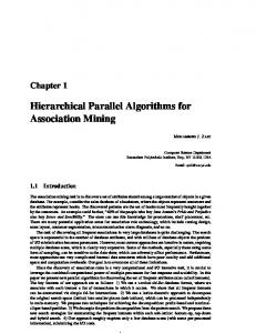
In Step 1, we find A(DT C ) = A(D) ∪ {v1 v3 , v2 v5 , v1 v5 } (above right) and set D := DT C . Observe that v1 , v2 , v3 , v4 , v5 is an acyclic ordering. We may assume that this is the ordering found in Step 2. For i = 1 in Step 3, we have X = {v1 } and Y = {v2 , v3 , v4 , v5 } = N + (X), and we call B({v1 }, {v2 , v3 , v4 , v5 }). Then in Step 4, line 1, we compute A = {v2 , v3 , v4 , v5 } and then, at lines 3 and 4, obtain v = v5 , N − (v) = {v1 , v2 , v3 , v4 } and R = {v2 , v3 , v4 , v5 }. Then, at line 12, we make a recursive call to B(V (D), ∅). In this call we have A = B = ∅ so, at line 10, the set V (D) = {v1 , . . . , v5 } is output and the recursive call returns to line 13 of B({v1 }, {v2 , v3 , v4 , v5 }), where we make a call to B({v1 }, {v2 , v3 , v4 }). We are now effectively looking at the graph D1 below. ²¯ v1 ²¯ ³ ) ±° ³ v 2 @ R @ ®³ ²¯ ²¯ )³±° D1
v3
±°
v4
±°
²¯ v1 ²¯ ³ ³ ) ±° v 2 ®³ ²¯ )³±° v3 ±° D2
²¯ D3 v1 ²¯ ³ ) ±° ³ v2 ±°
In Step 4, lines 1-4, we compute A = {v2 , v3 , v4 } and obtain v = v4 , N − (v) = {v1 } and R = {v4 }. At lines 12 and 13 we make recursive calls to B({v1 , v4 }, {v2 , v3 }) and B({v1 }, {v2 , v3 }) respectively. In the call to B({v1 , v4 }, {v2 , v3 }), lines 1-4, we obtain v = v3 and R = {v2 , v3 }. This in turn generates calls to B({v1 , v4 , v2 , v3 }, ∅), which just outputs {v1 , v2 , v3 , v4 } and returns, and B({v1 , v4 }, {v2 }). The latter call generates calls to B({v1 , v4 , v2 }, ∅) and B({v1 , v4 }, ∅), which output {v1 , v2 , v4 } and {v1 , v4 }, respectively. In the call to B({v1 }, {v2 , v3 }), where we are effectively looking at D2 above, we obtain v = v3 and R = {v2 , v3 }. This in turn generates calls to B({v1 , v2 , v3 }, ∅), which just outputs {v1 , v2 , v3 } and returns, and B({v1 }, {v2 }) (graph D3 9
above). The latter call generates calls to B({v1 , v2 }, ∅) and B({v1 }, ∅), which output {v1 , v2 } and {v1 }, respectively. This completes the case i = 1 in Step 3, and all the cc-sets containing v1 have been output. Now we perform Step 3 with i = 2, effectively looking at the graph D4 . ²¯ v2 ³ ²¯ ²¯ ³ ) ±° v3 v4 B ±° BN HH ²¯ ©±° © j v5 © H ¼ ±°
D4
D5
²¯ v3
²¯ v4
±° HH ²¯ ©±° H j v5 © ¼© ±°
The call to B({v2 }, {v3 , v4 , v5 }) generates further recursive calls in the following order B({v2 , v5 , v3 }, {v4 }) B({v2 , v5 , v3 , v4 }, ∅), output {v2 , v3 , v4 , v5 } B({v2 , v5 , v3 }, ∅), output {v2 , v3 , v5 } B({v2 }, {v3 , v4 }) B({v2 , v3 }, {v4 }), output {v2 , v3 } B({v2 }, {v4 }), output {v2 }. Thus all the cc-sets containing v2 but not v1 are output. Performing Step 3 again with i = 3, effectively looking at the graph D5 above, the call to B({v3 }, {v4 , v5 }), generates the following recursive calls B({v3 , v5 }, {v4 }) B({v3 , v5 , v4 }, ∅), output {v3 , v4 , v5 } B({v3 , v5 }, ∅), output {v3 , v5 } B({v3 }, {v4 }), output {v3 } which output all the cc-sets containing v3 but not v1 or v2 . For the case i = 4 in Step 3 we get the following calls B({v4 }, {v5 }) B({v4 , v5 }, ∅), output {v4 , v5 } B({v4 }, ∅), output {v4 } and for i = 5 we get B({v5 }, ∅), output {v5 } after which A terminates. Recall that the cc-sets of D are precisely the cc- sets of DT C . For the rest of Section 3 D is assumed to be transitive as this holds after Step 1 of A. Lemma 3.2. Algorithm A correctly outputs all cc-sets of D. 10
Proof. Firstly we show that all the sets X output by A are in CC(D). We will show that within A, for any call B(X, Y ) we have that X ∩Y = ∅, X ∪Y is convex and X is a cc-set. This is clearly sufficient as X is the only set output. These properties hold for Step 3 when B({vi }, {vi+1 , . . . , vn }) is called as we have chosen an acyclic ordering of the vertices. Thus we assume that the properties hold for the sets X, Y and consider the pairs of sets X ∪ R, Y \R and X, Y \{v} constructed in B(X, Y ). In both cases clearly the intersections are empty, and since R ⊆ N + (X) ∪ N − (X), X ∪ R is connected. Now we will prove that X ∪ R is convex. Suppose that there is a path u, y, w where u, w ∈ X ∪ R, but y 6∈ X ∪ R. (Note that if there exists an (X ∪ R)path then by transitivity of D there exists an (X ∪ R)-path of length two.) By convexity of X ∪ Y we have y ∈ X ∪ Y . Also, y 6= v as y 6∈ R and v ∈ R. Assume that A 6= ∅. Then R ⊆ N + (X). Since u ∈ X ∪ N + (X) and the arc uy exists, the transitivity of D implies that y ∈ N + (X). Since X is convex it follows that not both vertices u, w can be in X and that there is no arc from N + (X) to X. Thus w 6∈ X and so w ∈ R ⊆ N − (v). By the transitivity of D and the fact that yw exists and that w ∈ N − (v) we have y ∈ N − (v) and thus y ∈ R, a contradiction. Similarly, we arrive at a contradiction when A = ∅, but B 6= ∅. Secondly we show that if S 6= ∅ is a cc-set, then S is output by A. If S is a cc-set and j = min{i : vi ∈ S} then {vj } ⊆ S ⊆ {vj , vj+1 , . . . , vn }. Thus it is sufficient to show that if S is cc and X ⊆ S ⊆ X ∪ Y then B(X, Y ) outputs S. We prove this by induction on |Y |. If N + (X) ∩ Y = ∅ = N − (X) ∩ Y then, since S is connected, S = X and B(X, Y ) outputs X at line 10. This proves the result for |Y | = 0, and, in addition, for |Y | ≥ 1 we may assume that v ∈ (N + (X) ∪ N − (X)) ∩ Y . If v 6∈ S then we have X ⊆ S ⊆ X ∪ (Y \{v}) and |Y \{v}| < |Y |, so by induction the call to B(X, Y \{v}) at line 13 outputs S. If r ∈ (R\{v}), we have arcs rv and xr, for some x ∈ X ⊆ S. Thus, if v ∈ S, by convexity of S we have R ⊆ S. Then, since |Y \R| < |Y |, the call to B(X ∪ R, Y \R) at line 12 outputs S. Lemma 3.3. Every cc-set of D is output at most once by A. The running time of A is O(n · cc(D)). Proof. Note that by Theorem 2.3 and the fact that D is connected we have 11
n × cc(D) ≥ n2 (n + 1)/2. Therefore the transitive closure of D can be found in O(n · cc(D)) time, by Theorem 2.2. It is well-known that an acyclic ordering can be found in time O(n + m), see, e.g., [4], and clearly the sets N + (v) and N − (v) can be computed at the start of the algorithm in O(n) time, for each v ∈ V (D). We will now show that B(X, Y ) runs in time O(|Y |·cc0 (X, Y )+KX,Y ), where cc0 (X, Y ) is the number of cc-sets S such that X ⊆ S ⊆ X ∪ Y and KX,Y is the sum of the sizes of the sets S. Note that B returns at line 10 or makes two recursive calls to B (lines 12,13). If B returns at line 10 then we call this a leaf call otherwise the function call is an internal call. All function calls can be viewed as nodes of a binary tree (every node is a leaf or has two children) whose leaves and internal nodes correspond to calls to B. It is easy to see, by induction, that the number of internal nodes equals the number of leaves minus one. It is easy to see, by induction on the depth of the call tree, that B outputs each set S only once (B(X ∪ R, Y \R) and B(X, Y \{v}) output those that contain v and do not contain v, respectively). Thus we have cc0 (X, Y ) leaf calls and cc0 (X, Y ) − 1 internal calls. In the next paragraph, we assume that the sets used by B(X, Y ) are implemented in a way that allows unit time insertion and deletion, and order-ofthe-set time searching. We also assume that the set implementation allows us to check whether a set is empty in unit time. A data structure satisfying the assumptions above is described in detail in Section 4.2. Also notice that the intersection of two sets P and Q can be found using deletions: P ∩ Q = Q \ (Q \ P ). The time taken by a call B(X, Y ) depends on the time taken to calculate the sets A, B and R. Since A, B ⊆ Y , the time to compute R is at most O(|Y |). By definition of R we have that N + (X ∪ R) = N + (X) − R and N − (X ∪ R) = N − (X) ∪ N − (v) − R − X provided A 6= ∅, and N − (X ∪ R) = N − (X) − R and N + (X ∪ R) = N + (X) ∪ N + (v) − R − X provided A = ∅ (and B 6= ∅). Since R ⊆ Y , these sets can be computed in O(|Y |) time. Then, if we implement B(X, Y ) so that N + (X) and N − (X) are passed in as parameters, the time taken to calculate A and B is at most O(|Y |). If B(X, Y ) calls B(X 0 , Y 0 ) then |Y 0 | < |Y | thus a call to B at an internal node takes at most O(|Y |) time, and a call at a leaf node takes at most O(|Y |+|X|) time, giving the desired total time bound of O(|Y | · cc0 (X, Y ) + KX,Y ). We let Ki denote the sum of the sizes of all the cc-sets S such that vi ∈ S ⊆ {vi+1 , . . . , vn }, and observe that K1 + . . . + Kn ≤ n · cc(D). 12
Finally, by Step 3, we conclude that the total running time is à n ! X cc0 ({vi }, {vi+1 , vi+2 , . . . , vn }) · (n − i) + Ki = O(cc(D) · n). O i=1
Theorem 3.4. Algorithm A is correct and its time and space complexities are O(n · cc(D)) and O(n2 ), respectively. Proof. The correctness and time complexity follows from the two lemmas above. The space complexity is dominated by the space complexity of Step 1, O(n2 ). Since cc(D) may well be exponential, we may wish to generate only a restricted number k of cc-sets. Theorem 3.5 can be viewed as a result in fixed-parameter algorithmics [7] with k being a parameter. Theorem 3.5. To output k cc-sets the algorithm A requires O(n2.376 + kn) time. Proof. We may assume that k is at most the number of cc-sets containing vertex v1 since otherwise the proof is analogous. We consider the binary tree T introduced in the proof of Lemma 3.3 and prove our claim by induction on k. It takes O(n2.376 ) time to perform Steps 1,2 and 3. It takes O(n) internal nodes of T to reach the first leaf of T and, thus, for k = 1 we obtain O(n2.376 + n) time. Assume that k ≥ 2. Let x be the first leaf of T reached by A, let y be the parent of x on T , let z be another child of y on T and let u be the parent of y. Observe that after deleting the nodes x and y and adding an edge between u and z, we obtain a new binary tree T 0 . By induction hypothesis, to reach the first k − 1 leaves in T 0 , we need O(n2.376 + (k − 1)n) time. To reach the first k leaves in T , we need to reach x and the first k − 1 leaves in T 0 . Thus, we need to add to O(n2.376 + (k − 1)n) the time required to visit x and y only, which is O(n). Thus, we have proved the desired bound O(n2.376 + kn).
13
4
Generating Convex Sets in Acyclic Digraphs
It is not hard to modify A such that the new algorithm will generate all convex sets of an acyclic digraph D in time O(n · co(D)), where co(D) is the number of convex sets in D. However, a faster algorithm is possible and we present one in this section. To obtain all convex sets of D (and ∅, which is not convex by definition), we call the following recursive procedure with the original digraph D and with F = ∅. This call yields an algorithm whose properties are studied below. A vertex x is a source (sink) if it has no in-neighbors (out-neighbors). In general, the procedure CS takes as input an acyclic digraph D = (V, A) and a set F ⊆ V and outputs all convex sets of D which contain F . The procedure CS outputs V and then considers all sources and sinks of the graph that are not in F . For each such source or sink s, we call CS(D − s, F ) and then add s to F . Thus, for each sink or source s ∈ V \ F we consider all sets that contain s and all sets that do not contain s. CS(D = (V, A), F ) 1.
output V ; set X := V \ F
2.
for all s ∈ X with |N + (s)| = 0 or |N − (s)| = 0 do {
3.
+ − for all v ∈ V find ND−s (v) and ND−s (v)
4.
call CS(D − s, F ); set F := F ∪ {s}
5.
+ − for all v ∈ V find ND (v) and ND (v)
4.1
}
Correctness of the Procedure
Proposition 4.2 and Theorem 4.3 imply that the procedure CS is correct. We first show that all sets generated in line 1 are, in fact, convex sets. To this end, we use the following lemma. Lemma 4.1. Let D be an acyclic graph, let X be a convex set of D, and let s ∈ X be a source or sink of D[X]. Then X \ {s} is a convex set of D. Proof. Suppose that X \{s} is not convex in D. Then there exist two vertices u, v ∈ X \ {s} and a directed path P from u to v which contains a vertex not 14
in X \ {s}. Since X is convex, P only uses vertices of X and in particular s ∈ P . Thus, there is a subpath u0 sv 0 of P with u0 , v 0 ∈ X. But since s is a source or a sink in D[X] such a subpath cannot exist, a contradiction. Now we can prove the following proposition. Proposition 4.2. Let D = (V, A) be an acyclic digraph and let F ⊆ V . Then every set output by CS(D, F ) is convex. Proof. We prove the result by induction on the number of vertices of the output set. The entire vertex set V is convex and is output by the procedure. Now assume all sets of size n − i ≥ 2 that are output by the procedure are convex. We will show that all sets of size n − i − 1 that are output are also convex. When a set C is output the procedure CS(D[C], F 0 ) was called for some set F 0 ⊆ V . The only way CS(D[C], F 0 ) can be invoked is that there exist a set C 0 ⊂ V and a source or sink c of D[C 0 ] with C = C 0 \ {c}. Moreover C 0 will be output by the procedure and, thus, by our assumption is convex. The result now follows from Lemma 4.1. Theorem 4.3. Let D = (V, A) be an acyclic digraph and let F ⊆ V . Then every convex set of D containing F is output exactly once by CS(D, F ). Proof. Let C be a convex set of D containing F . We first claim that there exist vertices c1 , c2 , . . . , ct ∈ V with V = {c1 , c2 , . . . , ct }∪C and ci is a source or sink of D[C ∪ {ci , ci+1 , . . . , ct }] for all i ∈ {1, 2, . . . , t}. To prove the claim we will show that for every convex set H with C ⊂ H ⊆ V , there exists a source or sink s ∈ D[H \ C] of the digraph D[H]. This will prove our claim as by Lemma 4.1 H \ {s} is a convex set of D and we can repeatedly apply the claim. If there exists no arc from a vertex of C to a vertex of D[H \ C] then any source of H \C is a source of D[H]. Note that D[H \C] is an acyclic digraph and, thus, has at least one source (and sink). Thus we may assume that there is an arc from a vertex u of C to a vertex v of H \ C. Consider a longest path v = v1 v2 . . . vr in D[H \ C] leaving v. Observe that vr is a sink of D[H \ C] and, moreover, there is no arc from vr to any vertex of C since otherwise there would be a directed path from u ∈ C to a vertex in C containing vertices in H \ C which is impossible as C is convex. Hence vr is a sink of D[H] and the claim is shown.
15
Next note that a sink or source remains a sink or source when vertices are deleted. Thus when CS(D, F ) is executed and a source or sink s is considered, then we distinguish the cases when s = ci for some i ∈ {1, 2, . . . , t} or when this is not the case. If s = ci and we currently consider the digraph D0 and the fixed set F 0 , then we follow the execution path calling CS(D0 −s, F 0 ). Otherwise we follow the execution path that adds s to the fixed set. When the last ci is deleted, we call CS(D[C], F 00 ) for some F 00 and the set C is output. It remains to show that there is a unique execution path yielding C. To see this, note that when we consider a source or sink s then either it is deleted of moved to the fixed set F . Thus every vertex is considered at most once and then deleted or fixed. Therefore each time we consider a source or sink there is a unique decision that finally yields C.
4.2
Running time of CS
We will use the following data structure for a set Y = {y1 , y2 , . . . , y|Y | } ⊆ {1, 2, . . . , n} that supports unit time element insertion and deletion, unit time checking whether Y is empty, and allows us to iterate over the elements of Y in O(|Y |) time. We maintain arrays of integers succ and pred indexed from 0 to |Y | where succk = k and predk = k if and only if k 6∈ Y . If Y = ∅ then pred0 = succ0 =0. If Y 6= ∅ then predyi holds yi−1 for every i ≥ 2 and 0 for i = 1, and succyi holds yi+1 for every i < |Y | and 0 for i = |Y |. We can iterate over the elements of V by following the chain of links from succ0 . Notice that succ0 holds y1 and pred0 holds y|Y | . We can initialize this structure to an empty set by setting all elements succi and predi to i, and we can initialize Y := {1, 2, . . . , n} by setting all elements succi and predi to i + 1 mod n + 1 and i − 1 mod n + 1, respectively. By analogy with conventional doubly-linked list insertion and deletion, we have: insert(k) succk := 0 predk :=pred0 succpred0 := k pred0 := k
delete(k) succpredk := succk predsucck := predk predk := k succk := k
+ − We can use this data structure for sets V , X, ND (v), ND (v), v ∈ V , and
16
F for the input acyclic digraph D = (V, A) of order n. We can initialize the data structures for all these sets in time O(n2 ) using, say, the adjacency matrix of D. Observe that we output the vertex set of D as one convex set. Thus, it suffices to show that the running time of CS(D, F P) without the recursive calls is O(|V |). This will yield the running time O( C∈CO(D) |C|) of CS by Theorem 4.3. Using our data structure, we can determine all sources and sinks in O(|V |) time. For the recursive calls of CS we delete one vertex and have to update the number of in-, respectively, out-neighbors of all neighbors of the deleted vertex s by iterating over V. The vertex s has at most |V | − 1 neighbors and we can charge the cost of the updating information to the call of CS(D − s, F ). Moreover we store the neighbors of s so that we can reintroduce them after the call of CS(D − s, F ). Moving the sinks and sources to F needs constant time for each source or sink and thus we obtain O(|V |) time in total. In summary we initially need O(n2 ) time, and then each call of CS(D, F ) is charged with O(|V |) before it is called and then additionally with O(|V |) time during its execution. Since wePoutput a convex setPof size O(|V |), the total running time is O(n2 ) + O( C∈CO(D) |C|). Since C∈CO(D) |C| = P Ω(n2 ) by Theorem 2.3, the running time of CS is O( C∈CO(D) |C|).
5
Implementation and Experimental Results
In order to test our algorithms A and CS for practicality we have implemented and run them on several instances of DDG’s of basic blocks. We have compared our algorithms with the state-of-the-art algorithm of Chen, Maskell and Sun [5] (the CMS algorithm) using their own implementation, but with the code for I/O constraint checking removed so as to ensure that their algorithm was not disadvantaged. For completeness we have also compared CS to Atasu, Pozzi and Ienne’s algorithm [17] (the API06 algorithm). All the algorithms were coded in C++ and all experiments were carried out on a 2 x Dual Core AMD Opteron 265 1.8GHz processor with 4 Gb RAM, running SUSE Linux 10.2 (64 bit). Our first set of tests is based on C and C++ programs taken from the benchmark suites of MiBench [12] and Trimaran [20]. We compiled these benchmarks for both the Trimaran (A,B,C,D,E) and SimpleScalar [3] (F,G,H,I) 17
ID A B C D E F G H I
NV 35 42 26 39 45 24 20 20 43
NA 38 45 28 94 44 22 19 21 47
NS 139,190 4,484,110 5,891 3,968,036 1,466,961 46,694 397 1,916 10,329,762
CMS (CT) 170 5,546 6 4,346 1,750 60 0 0 13,146
A (CT) 96 3,246 4 2,710 1,156 30 0 0 7,210
Table 1: All convex sets for benchmark programs architectures. From here we examined the control-flow graph for each program to select a basic block within a critical loop of the program (often this block had been unrolled to some degree to increase the potential for efficiency improvements). We considered basic blocks, ranging from 20 to 45 lines of low level, intermediate code, for which we generated the DDGs. We then selected, from these DDGs, the non-trivial connected components on which to run our algorithms. We give some preference to benchmarks which suit the intended application of the research taking our test cases from security applications including benchmarks for the Advanced Encryption Standard (B,C) and safety-critical software (A, E). We also include a basic example from the Trimaran benchmark suite: Hyper (D), an algorithm that performs quick sort (F), part of a jpeg algorithm (G), and an example from the fft benchmark in mibench containing C source code for performing Discrete Fast Fourier Transforms (H). The final example is taken from the standard blowfish benchmark, an encryption algorithm. The results we have obtained are given in Table 1. In the following tables NV denotes the number of vertices, NS denotes the number of generated sets, NA number of arcs, CT denotes clock time in 10−3 CPU seconds, and for the benchmark data ID identifies the benchmark. For examples G and H both algorithms ran in almost 0 time. For the other examples, the above results demonstrate that our algorithm A outperforms 18
NV 15 16 17 18 19 20 21 22
NA 56 64 72 81 90 100 110 121
NS 32,400 65,041 130,322 261,139 522,722 1,046,549 2,094,102 4,190,231
CMS (CT) 30 56 114 240 540 1,080 2,166 4,086
A (CT) 16 23 60 113 253 513 1,048 2,156
Table 2: cc-sets for graphs with maximum number of cc-sets the CMS algorithm. We also consider examples with worst-case numbers of cc-sets. Let, as in ~ p,q denote the digraph obtained from the complete bipartite Theorem 2.4, K graph Kp,q by orienting every edge from the partite set of cardinality p to ~ a,n−a with the partite set of cardinality q. By Theorem 2.4 the digraphs K |n−2a| ≤ 1 have the maximum possible number of cc-sets. Our experimental ~ a,n−a with |n − 2a| ≤ 1 are given in Table 2. Again results for digraphs K we see that A outperforms the CMS algorithm. We have compared algorithm CS with both CMS running in ‘unconnected’ mode and with API06. The examples used are the same as in Table 1, however we do not give results for examples B, D, E and I as these graphs produce an extremely large number of convex sets and as a result, do not terminate in reasonable time. The results are shown in Table 3. We can see that although CMS generally out-performs API06, there are two cases where API06 is marginally better. However, CS is consistently three to five times faster than either of the other algorithms. For interest we have also compared API06, CMS and CS on the digraphs that have maximal numbers of cc-sets. The results are shown in Table 4. Again, while CMS and API06 are roughly comparable, CS is a least twice as fast as both of them.
19
ID A C F G H
NV 35 26 24 20 20
NA 38 28 22 19 21
NS 1,123,851 120,411 3,782,820 122,111 55,083
API06 2,560 250 3,250 70 110
CMS (CT) 1,390 120 3,630 120 110
CS (CT) 570 40 1840 50 20
Table 3: All convex sets for benchmark programs
NV 15 16 17 18 19 20 21 22
NA 56 64 72 81 90 100 110 121
NS 32,768 65,536 131,072 261,144 524,288 1,046,575 2,097,152 4,194,304
API06 40 70 140 320 720 1,590 3,320 7,140
CMS (CT) 40 70 130 320 700 1,500 3,010 6,310
CS (CT) 10 30 60 130 250 550 1,070 2,190
Table 4: All convex sets for graphs with maximum number of cc-sets
20
6
Discussions
Our computational experiments show that A performs well and is of definite practical interest. We have tried various heuristic approaches to speed up the algorithm in practice, but all approaches were beneficial for some instances and inferior to the original algorithm for some other instances. Moreover, no approach could significantly change the running time. The algorithm was developed independently from the CMS algorithm. However, the two algorithms are closely related, and work continues to isolate the implementation effects that give the performance differences. Acknowledgements. We are grateful to the referees for a number of suggestions that allowed us to significantly improve the paper. We are grateful to the authors of [5] for helpful discussions and for giving us access to their code allowing us to benchmark our algorithm against theirs. Research of Gregory Gutin and Anders Yeo was supported in part by an EPSRC grant. Research of Gutin was also supported in part by the IST Programme of the European Community, under the PASCAL Network of Excellence, IST2002-506778.
References [1] ARM, www.arm.com [2] K. Atasu, L. Pozzi and P. Ienne, Automatic application-specific instruction-set extensions under microarchitectural constraints. In Proc. 40th Conf. Design Automation, ACM Press (2003), 256–261. [3] T. Austin, E. Larson and D. Ernst, SimpleScalar: An Infrastructure for Computer System Modeling. Computer 35 (2002), 59–67. [4] J. Bang-Jensen and G. Gutin, Digraphs: Theory, Algorithms and Applications. Springer-Verlag, London, 2000, 754 pp. [5] X. Chen, D.L. Maskell, and Y. Sun, Fast identification of custom instructions for extensible processors. IEEE Trans. Computer-Aided Design Integr. Circuits Syst. 26 (2007), 359–368.
21
[6] D. Coppersmith and S. Winograd, Matrix multiplication via arithmetic progressions. In Proceedings of the 19th Ann. ACM Symp. on Theory of Computation (1987), 1–6. [7] R.G. Downey and M.R. Fellows, Parameterized Complexity, Springer– Verlag, New York, 1999. [8] M.J. Fisher an A.R. Meyer, Boolean matrix multiplication and transitive closure. In Proceedings of the 12th Ann. ACM Symp. on Switching and Automata Theory (1971), 129–131. [9] M.E. Furman, Application of a method of fast multiplication of matrices in the problem of finding the transitive closure of a graph. Sov. Math. Dokl. 11 (1970), 1252. [10] H.N. Gabow and E.W. Myers, Finding All Spanning Trees of Directed and Undirected Graphs. SIAM J. Comput. 7 (1978), 280–287. [11] G. Gutin and A. Yeo, On the number of connected convex subgraphs of a connected acyclic digraph. Submitted. [12] M. R. Guthaus, J. S. Ringenberg, D. Ernst, T. M. Austin, T. Mudge and R. B. Brown, MiBench: A free, commercially representative embedded benchmark suite, In Proceedings of the WWC-4, 2001 IEEE International Workshop on Workload Characterization, (2001), 3–14. [13] S. Kapoor and H. Ramesh, Algorithms for enumerating all spanning trees of undirected and weighted graphs. SIAM J. Comput. 24 (1995), 247–265. [14] D.L. Kreher and D.R. Stinson, Combinatorial Algorithms: Generation, Enumeration and Search, CRC, 1999. [15] G.J. Minty, A simple algorithm for listing all trees of a graph. IEEE Trans. Circuit Theory CT-12 (1965), 120. [16] MIPS, www.mips.com [17] L. Pozzi, K. Atasu and P Ienne, Exact and approximate algorithms for the extension of embedded processor instruction sets. IEEE Trans. on CAD of Integrated Circuits and Systems, 25 (2006), 1209–1229. [18] R.C Read and R.E Tarjan, Bounds on backtrack algorithms for listing cycles, paths, and spanning trees. Networks 5 (1975), 237–252. 22
[19] Tensilica, www.tensilica.com [20] The Trimaran Compiler Infrastructure, www.trimaran.org [21] A. Shioura and A. Tamura, Efficiently scanning all spanning trees of an undirected graph. J. Operation Research Society Japan 38 (1995), 331–344. [22] A. Shioura, A. Tamura and T. Uno, An optimal algorithm for scanning all spanning trees of undirected graphs. SIAM J. Comput. 26 (1997), 678–692. [23] T. Uno, A new approach for speading up enumeration algorithms. Proc. ISAAC’98, Lecture Notes Computer Sci. 1533 (1998), 287–296. [24] P. Yu and T. Mitra, Satisfying real-time constraints with custom instructions. CODES+ISSS ’05: Proceedings of the 3rd IEEE/ACM/IFIP international conference on Hardware/software codesign and system synthesis, ACM, New York (2005), 166–171.
23