Mar 1, 2015 - For safety reasons, movement of ships on the sea must be monitored. What is more, the real time vessel tracking is not enough. Those data ...
http://www.transnav.eu
the International Journal
Volume 9
on Marine Navigation
Number 1
and Safety of Sea Transportation
March 2015 DOI: 10.12716/1001.09.01.09
Algorithms for Ship Movement Prediction for Location Data Compression A. Czapiewska & J. Sadowski Faculty of Electronics, Telecommunications and Informatics, Gdansk University of Technology, Poland
ABSTRACT: Due to safety reasons, the movement of ships on the sea, especially near the coast should be tracked, recorded and stored. However, the amount of vessels which trajectories should be tracked by authorized institutions, often in real time, is usually huge. What is more, many sources of vessels position data (radars, AIS) produces thousands of records describing route of each tracked object, but lots of that records are correlated due to limited dynamic of motion of ships which cannot change their speed and direction very quickly. In this situation it must be considered how many points of recorded trajectories really have to be remembered to recall the path of particular object. In this paper, authors propose three different methods for ship movement prediction, which explicitly decrease the amount of stored data. They also propose procedures which enable to reduce the number of transmitted data from observatory points to database, what may significantly reduce required bandwidth of radio communication in case of mobile observatory points, for example onboard radars.
1 INTRODUCTION For safety reasons, movement of ships on the sea must be monitored. What is more, the real time vessel tracking is not enough. Those data should be stored and available for future use by authorized institutions. Unfortunately, the number of vessels seen near the coast is huge. Furthermore, the sources from which the information about vessels trajectories can be possessed are also few – AIS, radars, mobile observatory points – and each of them gives thousands of records describing route of each tracked object. However, one must ask if all those data are really important and provide significant update in the knowledge of position, speed or state of vessels. Most of ships which are moving on Baltic Sea are following known routs. In addition, because of their dimensions their dynamic is limited. They cannot change their speed and direction very quickly. That makes a
possibility to predict some parts of the routs on the basis of current parameters of motion to reduce the amount of data stored in databases. In this paper authors propose three different methods for ship movement prediction. Performance of these methods was tested on the basis of real vessels’ tracks gathered from AIS receiver. Authors also propose procedures responsible for selection of data records which must be stored because they provide significant update of position or velocity parameters. Those procedures may also be used in observatory points such as buoys or border guard vessels which send information by radio links with limited bandwidth. Described procedures will significantly reduce the number of transmitted data from those objects. Which in turn will reduce the time of transmission and may save radio communication resources.
75
This paper is divided into two parts. In the first one proposed algorithms are presented. In the second part the results of comparison analysis are shown.
2 ALGORITHMS FOR SHIP MOVEMENT PREDICTION In literature there are many methods used for prediction and system modelling, to mention few: an autoregressive model AR, a moving average model AM or an autoregressive moving average model ARMA. They are described i.e. in Kashyap (1982), Grenier (1983) or Al‐Smadi (2009). In those methods parameters of models must be established. Many publications are devoted to the problem of settlement of those parameters as it is unique problem for different models and systems. Therefore, in this paper authors propose to use the simplest descriptions of ship movement: linear and circular. They compare the performance of those two movement descriptions with well‐known however complex Kalman filtering estimation method. In the paper authors proves that for ship movement prediction the simplest model description is efficient and sufficient. Thus, three different algorithms designed for movement prediction of vessels tracks are discussed in this paper. Because most of the ships are moving by the shortest route we may assume that they are moving along rather linear path. That is why, first algorithm is based on the monotonous, linear movement description and it will be later called a linear algorithm. Second algorithm assumes that, while vessels cannot do sharp turns, they must follow arcs. So their trajectories may by described by a part of the circle. This algorithm is called in this paper a circle algorithm. The last algorithm is the most complex one considering those three. It uses Kalman filtering. Authors made also some assumptions about system that might use those algorithms. They presumed that vessels trajectories data would be gathered by some remote observatory points (sensors) connected to central database via radio links. To reduce the amount of transmitted data, one of the algorithms mentioned above will be used. Prediction of vessels’ tracks must be performed on the both sides of data communication channel: central data base (central server) will calculate coordinates of vessels between records of true positions received from remote sensors; remote sensors will perform the same prediction in order to decide if the real coordinates of vessels differ from estimated/predicted ones by more than specified threshold. It is obvious, that the amount of data which will have to be transmitted and stored in database will depend on the required accuracy of route estimation (the established threshold). Authors also assumed that the basic source of information about vessels would be Automatic Identification System AIS (IMO (1998)) system 76
(Automatic Identification System) and information from this system were used to conduct comparative analysis.
2.1 Linear algorithm Every vessel through AIS system sends information about its movement: if it is moving or not, its speed over ground (SOG), its direction of movement COG (Course Over Ground), and current position. If the position of vessel is given in Cartesian coordinate system (not in WGS‐84 coordinates) the next position might be estimated as follows. Firstly, the speed given in knots (SOG) should be converted to m/s (sog) with equation:
sog 0,514444 * SOG .
(1)
Then the overall shift s in time t of the moving object must be calculated:
s sog t .
(2)
To calculate the shift in x and y axis (respectively
x and y ) the course COG of the vessel must be taken into account:
x s sin COG / 180 . y s cosCOG / 180
(3)
Finally, new coordinates of the object are:
x' x x . y ' y y
(4)
The x and y are coordinates of the object in previous moment. Those values must be known ‐ from AIS system or from previous estimations if the errors of those estimation are smaller than established threshold.
2.2 Circle algorithm Circle algorithm should be better to describe movements of maneuvering vessel. In this algorithm the main assumption is that ships have huge inertia what makes them disable to perform quick direction or speed changes. The direction is usually changed on arc trajectory. To write equation of particular circle one must know the coordinates of circle center (a,b) and its radius r. To find those parameters knowledge of coordinates of three points ((x1, y1), (x2, y2) and (x3, y3)) lying on the circumference is needed. Than a system of equations can be written:
a 2 2ax1 x12 y12 2by1 b 2 r 2 0 2 2 2 2 2 a 2ax2 x2 y2 2by2 b r 0 . a 2 2ax x 2 y 2 2by b 2 r 2 0 3 3 3 3
(5)
From above equations the parameters of the circle can be found. At first, those equations must be rewritten to:
a c b d ,
2 B 2b 2 A 2a r 2 R 2 a 2 A2 b 2 B 2 D 2 A 2a 2 E C 1
C
(6)
(10)
F 2CD 2aC 2b G D 2 2aD a 2 b 2 r 2 one can get:
where
x Cy D . 2 y E yE G 0
y y3 c 1 , x3 x1 x32 x12 y12 y32 ; 2 x3 x1 2d x2 x1 e , b 2cx2 x1 y2 y1
(11)
As a result of above calculations two points lying on the circle are found. To decide which one is the correct one the COG parameter might be used.
d
(7)
where
While implementing this algorithm one must be aware that not for every three points system of equations (5) is solvable. In that case it is recommended to use linear algorithm for such three points.
e x12 x22 y12 y22 . Then to find value of circle radius the circular equation might be used. When the speed of object is known the length of the arc s passed by the object in time t can be found from equation (2). Symbols used in following equations are explained in Figure 1. As we know the value of s and r, the angle and value of R can be calculated from:
s 360 2 r
R 2 r sin
.
Figure 1. Explanation of symbols used in Equation (8) – (11).
2
Then two circle equations might be written. One with center in (a, b) and radius r. The other with center in (A, B) and radius R:
r 2 x a 2 ( y b) 2 . 2 2 2 R x A ( y B )
(8)
(9)
Modifying above system of equations and using beneath symbols:
2.3 Kalman filtering Kalman filtering is an recursive algorithm which provides means to estimate the state of discrete linear dynamic process in such a way that it minimizes the mean of the squared error (Welch & Bishop 2006). It means that Kalman filtering may be used for ship movement estimation. The following equations were written basing on the theory found in mentioned Welch & Bishop (2006) and Grewal & Andrews (2008). The state vector is:
x y x , v x v y
(12)
77
where x, y represents position coordinates of the object and vx, vy are values of linear speed in x and y axis. Speed values depends from SOG and COG. The transition matrix for this state vector is:
1 0 A 0 0
0 1 0 0
0 t , 0 1
t 0 1 0
(13) 3 COMPARATIVE ANALYSIS
where t is time difference between current measurement and previous one. The process noise covariance matrix is a diagonal one Q = Iq, where I is identity matrix and q must be a positive value. The measurement noise covariance matrix is calculated in every recursion:
rx 0 R 0 0
0
0
ry
0
0 0
rvx 0
When the distance between estimated position and true position is greater than established threshold the true position must be remembered and also send to database center. What is more, in next filter recursion, it is forbidden to use the estimated state vector. As a state vector must be used remembered measurement (true position).
0 0 , 0 rvy
(14)
where diagonal values are variances of last three measurements of x, y and vx, vy. Matrix H that relates the state to the measurement vector is an identity matrix, as elements of state vector and measurement vector are the same. Procedures of Kalman filtering are conducted in two phases. In first one, a prediction phase, the state vector and a priori estimate error covariance is updated:
To perform a comparative analysis of presented algorithms data from AIS system were recorded. A receiving AIS antenna was placed on the roof of the building of Faculty of Electronics, Telecommunications and Informatics of Gdansk University of Technology. Location of antenna and sensitivity of receiver allowed to record AIS data from all vessels in the Bay of Gdansk. Duration time of recording was approximately one hour. For comparative analysis were used only records of vessels that were moving. Information about ship movement is send as navigational status in AIS system. All algorithms were executed on data converted from WGS84 coordinate system to PUWG2000 coordinate system. For each algorithm were determined: estimated route, number of positions gathered by AIS system (true positions), number of positions that must be stored in database, root mean square error for each trajectory. Results achieved for three vessels are discussed in paragraphs 3.1 – 3.3. In paragraph 3.4 there is shown analysis for all moving ships recorded within an hour.
3.1 Vessel MMSI 212425000
x Ax P A P AT Q
.
(15)
In second phase, a correction one, Kalman gain K is calculated and state vector as well as error covariance matrix are corrected:
K P HT H P HT R
x x K z H x P I K H P
1
.
(16)
During the following comparative analysis, it was assumed that the initial state vector of Kalman filter consists of the oldest measurements (those with the smallest timestamp). While the first measurement vector consists of measurements with the second smallest timestamp. Because there are needed three measurements to fill measurement noise covariance matrix first three iterations of Kalman filtering do not return any result. Those three measurements must always be remembered and send to database center.
78
This object was moving towards harbor in Gdynia. Its dimensions are 185x30 m and its draught is 10.9 m. In Tables 1‐4 are presented results for different thresholds. There are root mean square errors for path calculated with utilization of all positions (RMS of all positions) and calculated only for estimated positions (RMS of estimated positions). In the last column is information about the number of remembered points given in percentage. The number of all points for this vessel is 616 (length of trajectory is several kilometers). Table 1. Results for vessel MMSI 212425000 and threshold equal to 10 m. _______________________________________________ Algorithm RMS of RMS of Stored estimated positions _______ positions all positions _________ _______________ _______________________________________________ m m % Linear 4.8 5.1 10.8 Circle 4.6 4.9 11.7 Kalman 4.8 5.1 11.2 _______________________________________________
Table 2. Results for vessel MMSI 212425000 and threshold equal to 50 m. _______________________________________________
Table 7. Results for vessel MMSI 235000193 and threshold equal to 100 m. _______________________________________________
Algorithm RMS of RMS of Stored estimated positions _______ positions all positions _________ _______________
Algorithm RMS of RMS of Stored estimated positions _______ positions all positions _________ _______________
_______________________________________________ m m %
_______________________________________________ m m %
Linear 23.2 23.7 4.2 Circle 23.6 24.2 5.2 Kalman 23.3 23.8 4.5 _______________________________________________
Linear 42 46 15.6 Circle 58 60 4.2 Kalman 61 61 2.1 _______________________________________________
Table 3. Results for vessel MMSI 212425000 and threshold equal to 100 m. _______________________________________________ Algorithm RMS of RMS of Stored estimated positions _______ positions all positions _________ _______________
As it can be seen for this particular object and trajectory linear algorithm gives the worst results, especially for large value of threshold. However, only for this case the linear algorithm performs so poorly.
_______________________________________________ m m % Linear 47 48 3.4 Circle 41 42 3.6 Kalman 46 46 3.6 _______________________________________________ Table 4. Results for vessel MMSI 212425000 and threshold equal to 200 m. _______________________________________________ Algorithm RMS of RMS of Stored estimated positions _______ positions all positions _________ _______________ _______________________________________________ m m % Linear 80 80 2.1 Circle 93 94 2.6 Kalman 77 78 2.3 _______________________________________________
For this particular vessel all of the algorithms gave similar results. Nevertheless, they allowed to reduce number of stored data significantly.
3.3 Vessel MMSI 244482000 This object was also moving towards harbor in Gdansk. Its dimensions are 83x12 m and its draught is 3.6 m. This vessel, in spite of navigational status suggesting that it was moving, was maneuvering to moor in Kaszubian Canal, what can be seen in Figure 2. Nevertheless, all of the discussed algorithms were executed for this object. Results are shown in Tables 8 and 9 as in previous cases. For this vessel also all of the algorithms performed equally. The root mean square errors are similar as well as the number of data that must be remembered in database. However, as the ship was maneuvering in space of few meters with very low speed, this is one of the easiest cases to estimate the route.
3.2 Vessel MMSI 235000193 This vessel was moving towards Gdansk. Its dimensions are 80x13 m and its draught is 6.6 m. For this object only 96 points were recorded that allowed to recall trajectory of length about 170 m. In Tables 5 – 7 are shown results for different thresholds as it was shown in previous paragraph. Table 5. Results for vessel MMSI 235000193 and threshold equal to 10 m. _______________________________________________ Algorithm RMS of RMS of Stored estimated positions _______ positions all positions _________ _______________ _______________________________________________ m m % Linear 3.3 4.8 53.1 Circle 4.4 5.1 26.0 Kalman 3.2 4.7 54.2 _______________________________________________
Table 6. Results for vessel MMSI 235000193 and threshold equal to 50 m. _______________________________________________ Algorithm RMS of RMS of Stored estimated positions _______ positions all positions _________ _______________ _______________________________________________ m m % Linear 25.1 28.4 21.9 Circle 20.0 20.7 7.3 Kalman 26.5 29.8 21.9 _______________________________________________
Figure 2. Points of route of vessel MSSI 244482000.
Table 8. Results for vessel MMSI 244482000 and threshold equal to 10 m. _______________________________________________ Algorithm RMS of RMS of Stored estimated positions _______ positions all positions _________ _______________ _______________________________________________ m m % Linear 5.2 5.5 9.2 Circle 5.3 5.6 9.6 Kalman 5.3 5.5 9.4 _______________________________________________
79
Table 9. Results for vessel MMSI 244482000 and threshold equal to 50 m. _______________________________________________ Algorithm RMS of RMS of Stored estimated positions _______ positions all positions _________ _______________ _______________________________________________ m m % Linear 7.1 7.1 0.1 Circle 7.1 7.1 0.4 Kalman 7.7 7.7 0.2 _______________________________________________
3.4 Comparison for all recorded vessels As it can be seen in above tables, the position prediction RMS error value is rather similar for all algorithms and strongly depends on established threshold of error estimation. For this reason, comparison for all recorded vessels was made only on the bases of number points that must be stored to fulfill the threshold condition. In Figures 3 – 6 are shown results for different thresholds. They are shown as column plots. On axis X are values of number of positions that must be remembered (in [%]) in ranges. Those ranges depends, of course, on the value of position prediction error threshold. On axis Y is the number of cases (also in [%]) in which the stored number of positions is within the particular range. As it can be seen all algorithms enables to significantly reduce the number of data that must be stored in memory to recall the vessel track. Even if the threshold is 10 m the amount of stored data for half of cases is less than 10%. For greater values of threshold the amount of points that must be remembered decreases rapidly to few percent for over a half of the cases. For threshold 100 m there is need to store only 5% of positions for 90% of cases. It proves the statement made in the introduction that the number of remembered points can be greatly reduced.
Figure 4. Stored positions for all algorithms for threshold 50 m.
Figure 5. Stored positions for all algorithms for threshold 100 m.
Figure 6. Stored positions for all algorithms for threshold 200 m.
Figure 3. Stored positions for all algorithms for threshold 10 m.
All of the algorithms give similar results. However, slightly better seem to be linear algorithm and the one using Kalman filtering over circular algorithm. As the linear algorithm is much less complex than Kalman filtering authors suggest using the linear one.
4 CONCLUSIONS As it was mentioned in the introduction, due to safety reasons, movement of vessels near the coast must be monitored. It is not enough to observe the situation on the sea in real time, but it is also important to have opportunity to store those data. However, the amount of data that concerns trajectories for each vessel 80
gathered only from AIS system is huge. The number of tracked objects is also significant. That means, there is an urgent need to have a possibility to reduce this amount of data. In this paper authors discuss algorithms that allows to reduce stored data to only few percent of the origin number and recall later the routes of the vessels with acceptable error. Those algorithms may be used not only to reduce stored data but also might be used to reduce data that must be send to central database from remote sensors. In that case, mentioned algorithms (or just one previously selected and used also on the receiver side) must be performed on the transmitter side. This feature is very important if observatory points use radio communication means for data transmission. The reduction of data will lead to spare radio resources by shortening the time of transmission or reducing the channel bandwidth.
REFERENCES Al‐Smadi A. M. 2009. Estimating autoregressive moving average model orders of non‐Gaussian processes, Proceedings of International Conference on Electrical and Electronics Engineering ELECO 2009, pages 133‐136 Grenier Y. 1983. Estimation of non‐stationary moving‐ average models, Proceedings of IEEE International Conference on ICASSP’83, volume 8, pages 268‐271 Grewal M. S., Andrews A. P. 2008. Kalman Filtering Theory and Practice using MATLAB IMO Resolution MSC.74(69). 1998. Kashyap R. L. 1982. Optimal Choice of AR and MA Parts in Autoregressive Moving Average Models, IEEE Transactions on Pattern Analysis and Machine Intelligence, pages 99‐104 Welch G., Bishop G. 2006. An Introduction to the Kalman Filter
*** This work was financially supported by Polish National Centre for Research and Development under grant no. O ROB/0022/03/001.
81