which builds a hierarchical query structure. Given a DTM. (. ) and two candidate points and , the "brute-force" approach reduces to computing the intersection of ...
Algorithms for Visibility Computation on Digital Terrain Models yLeila yUniversity
De Floriani,
yPaola
Magillo
of Genova, Computer and Information Science Department
Abstract In the paper, we consider the problem of computing visibility information on digital terrain models. Visibility problems on polyhedral terrains are classi ed according to the kind of visibility information computed into point visibility, line visibility and region visibility. A survey of the state-of-the-art of the algorithms for computing visibility is presented, according to the classi cation introduced.
Introduction Describing a terrain through visibility information, such as, for instance, the portion of the terrain surface visible from a selected point of view, has a variety of applications, such as geomorphology, navigation, terrain exploration. Problems which can be solved based on visibility are, for instance, the computation of the minimum number of observation points needed to view an entire region, the computation of paths with speci ed visibility characteristics, the computation of optimal location for the minimum number of television transmitters or the optimal locations for receivers [3, 4]. In terrain navigation problems, the pro le of the horizon is an ideal tool which can be used from an observer to locate his/her position on a map. In this paper, we consider the problem of computing visibility information on models of natural terrains. Two points on a terrain are considered mutually visible when they can be joined by a straight-line segment lying above the terrain (and intersecting it only at its two extreme points). We present a new classi cation of visibility problems based on the kind of visibility information computed. We consider point visibility problems, which consist of computing intervisibility between pairs of points, and produce discrete visibility models which
consist of collection of points selected in a candidate set which are visible from a prede ned set of observation points. Then, we examine visibility problems related to the computation of curves with speci ed visibility characteristics, like the horizon with respect to a point of view. Finally, we consider the problem of computing continuous visibility models, which require the computation of that portion of a terrain visible from a point of view located on the terrain (that we will call visibility model of the terrain with respect to the speci ed point of view). Visibility problems considered in this paper operate on the basis of a point of view located on the terrain (which will be termed Visibility on a terrain) to distinguish them from problems related to the visualization of a terrain, that we will call Visibility of a terrain. In this latter case, the point of view lies outside the domain of the terrain (possibly at in nity) and a projection plane (called a view plane) is given. The visibility problem of a terrain is related to the problem of computing the visible surfaces in a three-dimensional scene and has been extensively studied in the literature [20, 19, 14, 18, 15, 16, 5]. Moreover, some algorithms are more of a theoretical interest than of practical applicability. Here, we will focus on the problem of computing visibility on a terrain.
Digital terrain models A natural terrain can be described as a continuous function z = f (x; y), de ned over a connected subset D of the x 0 y plane. Thus, a Mathematical Terrain Model (MTM) can be de ned as a pair M � (D; f ).
P
A Digital Terrain Model (DTM) is de ned as a planar subdivision of the domain D into a collection of planar regions R= fR1; R2; . . . Rm g and by a family F of continuous functions z = fi (x; y), i = 1; 2; . . . m, each de ned on Ri and such that fi (x; y) = fj (x; y), for every (x; y) 2 Ri3 \ Rj3 (where Ri3 denotes the closure of region Ri). Thus, a DTM can be expressed as a pair M � ( ; F ).
P
According to the above de nition, a DTM is a special
case of mathematical terrain model. We will call face of a DTM the graph of each function fi , edge and vertex of the DTM the restriction of each function fi to an edge and a vertex, respectively, of . For simplicity, we will denote by o� the projection on the x 0 y plane of a generic geometric entity o in the 3D space.
P
DTMs can be classi ed into Regular Square Grids (RSGs), and Polyhedral Terrain Models (PTMs). In an RSG, the domain subdivision is a regular rectangular grid, while each function fi is a quadratic function obtained by linear interpolation along the edges of the subdivision. PTMs are characterized by a domain subdivision consisting of a straight-line plane graph and by linear interpolation functions. The graph of a polyhedral terrain model consists of a network of polygonal faces. A special class of PTMs is that consisting of Triangulated Irregular Networks (TINs), in which the domain subdivision is a triangulation. Often, a Delaunay triangulation is used as domain subdivision for a TIN because of its good behaviour in numerical interpolation problems [7]. A Delaunay triangulation has an important property related also to visibility computations. It belongs to the class of acyclic subdivisions of the plane, i.e., subdivisions on which it is possible to de ne a partial order relation, called before/behind relation, with respect to any point inside the domain of the subdivision [6]. A DTM based on an acyclic subdivision is called an acyclic digital terrain model. Such models have a special interest related to visibility application, since their faces and edges can be radially sorted around any pre xed point of view. In such a way, visibility information can be incrementally computed for each face or edge by only taking into account the con guration of the portion of the terrain formed by those faces and edges which come before them in the order, with a considerable increase in e�ciency.
Classi cation of visibility problems on terrains Given a mathematical terrain model M� (D; f ), that, for brevity, we will simply call a terrain, we call a candidate point any point P � (x; y; z ) belonging to or above the terrain, i.e., such that (x; y) 2 D and z � f (x; y). Two candidate points P1 and P2 are mutually visible (or intervisible) if, for every point Q � (x; y; z ) = tP1 + (1 0 t)P2, with 0 < t < 1, z > f (x; y). We will call point of view (or observation point) any arbitrarily chosen candidate point, and visual ray any ray emanating from a point of view. Given a point of view V and a spheric coordinate system centered at V , a visual ray r is identi ed by the pair (�; �), called a view direction, where � is the angle between the projection r � of r on the x 0 y plane and the positive x-axis, and � is the angle between r and the positive z -axis. Visibility problems on a terrain can be classi ed based on the dimensionality of their output information into
,
point line
and region
visibility
problems.
Point visibility Given a terrain, a point of view and a nite set Q of candidate points, we want to compute the subset Q0 of Q containing all the points visible from V . Q0 is called the discrete visible region of V in Q. In practice, we consider a DTM and the candidate points form a subset of the vertices of the terrain; often also the point of view is at a vertex. A generalization of the problem stated above consists of computing a discrete visibility model of a terrain. Given a terrain M, a nite set S1 of observation points, and a set S2 of points belonging to M, the discrete visibility model of M with respect to S1 and S2 is a collection of sets fQi j Pi 2 S1 g, where Qi = fP 2 S2 j P is visible from Vi g.
Line visibility The well-known visible-line reconstruction problem for general 3D scenes can be formulated as a line visibility problem for a terrain, by taking a point of view inside the domain, and requiring the computation of the visible portions of the edges of the DTM. A line visibility problem of practical relevance in geographic applications consists of computing the horizon of an observation point on a terrain. Given a terrain M and a point of view V , the horizon of the terrain with respect to V is a function � = h(�), de ned for � 2 [0; 2�] such that, for every radial direction �, h(�) is the maximum value � such that each ray emanating from V with direction (�; ), with < �, does not intersect the terrain. In a polyhedral terrain the horizon is a radially sorted list of labeled intervals [�1 ; �2]. If an interval [�1 ; �2] has label s, then the visual ray de ned by a direction (�; h(�)) with �1 < � < �2 hits the terrain at a point belonging to edge s. An example of horizon on a polyhedral terrain is represented in gure 1.
Region visibility Given a terrain M� (D; f ) and a point of view V , we de ne visible region of V the subset D0 of D formed by the points (x; y) 2 D such that (x; y; f (x; y)) is visible from V . The invisible region of V is clearly the complement of D0 in D. An example of visible and invisible region is shown in gure 2.
P
In a DTM M� ( ; F ), visibility with respect to a point of view can be coded as a map, called continuous visibility map, which consists of a partition of the domain D into maximal connected regions, each of which is labeled as invisible, if it is a subset of the invisible region, or with a face of the terrain in such a way that, if a region
R is labeled with face f , then all points of f whose vertical projection belongs to R are visible from the point of view. Given a set S of observation points, we call the collection of visibility maps of the points in S as the continuous visibility model of the terrain with respect to S .
9
Algorithms for point visibility
12
8
6
8
9
4 5
7
11 10 6
Point visibility computations can be reduced to determining the mutual visibility of two candidate points. In this section, we present a "brute-force" approach as well as an approach based on a preprocessing of the terrain which builds a hierarchical query structure.
P
Given a DTM M� ( ; F ) and two candidate points P1 and P2, the "brute-force" approach reduces to computing the intersection of the projection on the x 0 y plane of segment s � P1P2 , denoted s�, with the edges of . At each intersection point P� between s� and an edge e of , we test whether s lies above or below the edge of M corresponding to e. This process has a linear time complexity, in the worst case, in the number n of vertices of Mp . For a regular grid, the time complexity reduces to O( n). To compute the discrete visibility region with respect to a single point of view V , we need to determine the mutual visibility of V and the points belonging to a candidate set S2 .
P
P
7
Figure 1: Horizon of an observation point on a polyhedral terrain, projected on the x 0 y plane. The location of the view-point is the marked point.
The second approach preprocesses the terrain model with respect to the point of view V and builds a data structure on which the problem of computing the visibility of a point P from V can be solved in logarithmic time. The data structure has been proposed by Cole and Sharir [4] to solve a ray shooting problem on a polyhedral terrain.
P
7 10
9 6
10 V
4 1
Figure 2: An example of visible and invisible region on a TIN (the invisible region is shaded).
Given a DTM M� ( ; F ), a point of view V and a view direction (�; �), the ray shooting problem consists of determining the rst face of M hit by a ray emanating from V with direction (�; �). The mutual visibility of two points V and P reduces to solve the ray shooting problem, since we have just to consider as view direction that de ned by segment V P and, when obtained the rst face of M hit by the corresponding visual ray, we have just to determine whether P and V lie on the same or on opposite sides of the plane of such a face. The data structure of Cole and Sharir, that we call , has size O(n�(n) log n), where �(n) is the inverse of Ackermann's function, and thus almostconstant; ray shooting queries can be answered in time O(log2 n) on such structure. Given a point of view V , the horizon tree can be built for any acyclic polyhedral terrain, since it needs to sort the edges of the terrain around the viewpoint.
horizon tree
A horizon tree is a balanced binary tree in which the whole set of edges of the terrain is associated with the root. If S is the set of edges associated with a node v, then the closest half of the edges of S are associated with the left child of v, the other half with its right child. The partial horizon computed on the edges associated with the left child of a node v is attached to v. A horizon tree can be computed in optimal O(n�(n) log n) time. A ray shooting query, represented by a visual ray r, can be answered by descending the horizon tree T until two consecutive horizons are found such that the visual ray r passes above the rst one, but not above the second. This identi es two edges l1 and l2 of the DTM such that r passes above l1 , but below l2 . It can be proved that l1 and l2 bound the same face f , and that f is the rst face encountered by r. In descending T one node is visited at each level. For each node v the interval of the horizon associated with v containing ray r must be located. This leads to a time complexity of O(log2 n), which reduces to O(logn) by using a fractional cascading technique. Computing the discrete visible region of a model M with respect to a point of view V and a set S2 of k candidate points is thus equivalent to computing the horizon tree, with a computational cost equal to O(n�(n) log n), plus k intervisibility computations with a cost of O(klog2 n), which is clearly less than the direct intervisibility computation, if k = O(n).
Horizon computation algorithms The horizon computation problem reduces to the computation of the upper envelope of a set of possibly intersecting segments in the plane. Given p segments in the plane, i.e., p linear functions y = fi (x), i = 1 . . . p, each de ned on an interval [ai; bi], the upper
envelope
of such segments is a function
y = F (x), de ned over the union of the intervals [ai; bi], and such that F (x) = maxijx2[ai ;bi] (fi (x)). We express the edges of the terrain in a spherical coordinate system centered at the point of view and consider only the two angular coordinates. This transformation produces a set of segments in the � 0 � plane. By computing the upper envelope of such segments, we obtain a function which associates with each direction � the segment (if it exists) having maximum azimuth in direction �, i.e, the horizon (according to the given de nition). It has been shown [10] that the complexity of the upper envelope of p segments in the plane is O(p�(p)), and thus the complexity of the horizon of a polyhedral terrain with n vertices is equal to O(n�(n)). The upper envelope of p segments in the plane can be computed either by a dynamic, or by a divide-and-conquer approach. The dynamic approach computes the upper envelope, denoted Env, starting from an initially empty structure
and adding a segment at a time to it, in any order. For each new segment s, we locate those x-intervals, related to Env, which properly intersect the x-interval de ned by s, and update the upper envelope in each of these intervals. The worst-case time complexity of such algorithm is equal to O(p2). The rst divide-and-conquer algorithm for computing the upper envelope of a set of segments in the plane is due to Atallah [1] and achieves a worst-case time complexity of O(p�(p) log p). The algorithm recursively partitions the set of segments in two halves, and pairwise merges the results. The merging step of two upper envelopes is performed by using a sweep-line technique for intersecting two monotone chains of segments. The algorithm proposed by Hershelberg [13] is still based on a divide-and-conquer strategy, but computes the upper envelope of a set of p segments in optimal O(p log p) time. The basic idea is to subdivide the given set of segments in such a way that the upper envelope of any subset of the generated groups is linear in the number m of segments, and, thus, it can be computed in time O(m log m), by using the algorithm previously discussed. Since such subdivision generates O(log n) subsets, Atallah's algorithm is used to pairwise merge all partial envelopes according to a divide-and-conquer approach. This operation again has a O(p log p) time complexity, thus leading to O(p log p) time complexity for the entire algorithm in the worst case.
Algorithms for region visibility In this Section, we present rst a brief survey of algorithms for computing visibility of a terrain, i.e., for hidden surface removal on polyhedral terrains. Then, we describe in more detail speci c algorithms for computing a continuous visibility model, i.e., algorithms for visibility on a terrain.
Hidden surface removal on a polyhedral terrain The algorithms for hidden surface elimination in a 3D polyhedral scene (possibly a polyhedral terrain) give the visible portions of each object of the scene projected on the view plane, that form a visible image. The worst case space complexity of the visible image is O(n2 ) for a polyhedral scene with n vertices, but in practical cases its size may be much smaller. For this reason, output sensitive algorithms are more convenient than worst case optimal algorithms. In the following, we review some output sensitive algorithms for hidden surface elimination in polyhedral terrains, which can be adapted to the computation of a continuous visibility model. Reif and Sen [18] propose an output sensitive algorithm for hidden line elimination on acyclic polyhedral terrains, whose time complexity is equal to O((n + d) log2 n). The point of view is located at in nity in y direction, and the
x 0 z plane is used as view plane. The algorithm consists of two basic steps. In the rst step, the edges of the terrain are grouped to form O(n) monotone chains with respect to the y axis. In the second step, the chains are projected on the view plane one at a time, in increasing distance order. The upper envelope Env of the chains projected so far is maintained, representing the current horizon. When a chain � is projected, the intersections between � and Env are found. Then the portions of �, that lie above the current horizon Env, as visible from the viewpoint, are marked. Those portions of faces adjacent to the visible portions of the edges of �, and lying on the nearer side to the observation point are also visible. The update operation consists of the computation of the new horizon. A structure is used to store Env for representing monotone polygons. This makes possible to compute the intersections and the subsequent updatings in O((m + k) log m) time, where m is the number of edges and k the number of intersections. The same approach is followed by Preparata and Vitter [17], who, however, use a di�erent data structure for storing Env. The structure proposed by Preparata and Vitter is easier to implement, and consists of a subtree of the balanced binary tree whose leaves are the vertices of the terrain. The subtree is obtained by collecting only those leaves which correspond to vertices in Env. The structure allows intersections and updatings in O((m + k) log m) time, where m is the number of edges and k the number of intersections, thus leading to an O((n + d) log2 n) algorithm. De Berg, Halperin, Overmars, Snoeyink and Van Kreveld [5] proposep an output sensitive algorithm which works in O(n1+" d) time, where d is the output size, and " is any arbitrary integer value. The algorithm computes the visible image of a generic 3D scene composed of quasidisjoint triangular faces by using a sweepline technique (in particular, it can be applied to a TIN). A distance order is not required. The observation point is located at z = 01. The approach proposed by Katz, Overmars and Sharir [12] is more a "schema" of an algorithm, which can be applied to three-dimensional scenes formed by quasidisjoint objects sorted by increasing distance from a point of view (which can be in any position with respect to the scene: inside, outside or at in nity). In particular, the schema can be applied to an acyclic polyhedral terrain model, with observation point located on it. A description of this algorithm is presented in the subsection dedicated to continuous visibility algorithms.
Computing the lower envelope of a set of triangles An approach to the computation of the visibility model of a point of view on a digital terrain model consists of transforming the problem of computing the visibility
model into the problem of computing the lower envelope of a set of disjoint triangles in the space. The lower envelope of a set T of triangles in space de nes a partition of the x 0 y plane into maximal connected regions, each of which is labeled with a triangle of T in such a way that, if a region R is labeled with triangle t, then t is the triangle with minimum height over R. It has been shown [10] that such a partition has an O(n2 ) complexity (since all the triangles are disjoint). When computing the visibility model with respect to a point of view V , we associate as "height" to a triangle ti a function fi (x; y) that maps into a point P� � (x; y) in the plane the distance from V of the point P on ti whose projection on the plane is P� . The same approach could be used for hidden surface removal on a terrain, provided that the projection plane is the view plane. The algorithms, which compute the upper envelope Env(T ), compute a rst ner subdivision, denoted A(T ), obtained by projecting all the triangles on the x 0 y plane and extending the projected segments to in nity. A(T ) has still an O(n2 ) complexity and is formed only by convex regions. A "brute force" approach to determine A(T ) consists of computing for each region R, the triangle whose "height" is minimum with respect to the values of all the "height" functions associated with the triangles overlapping R. The worst case time complexity would be O(n3 ), since the projection of n triangles can cover a single region. An optimal approach to computing the lower envelope of a set of triangles has been proposed by Edelsbrunner, Guibas and Sharir [9]. Such algorithm is based on the classical divide-and-conquer paradigm, since it recursively partitions set T in two equally-sized subsets T1 and T2 , separately builds A(T1 ) and A(T2 ), and, nally, merges A(T1 ) and A(T2 ) into A(T ) by reassigning the labels in the regions at which A(T1 ) and A(T2 ) intersect. The worst case time complexity of the algorithm is equal to O(n2); Env(T ) can be computed from A(T ) in O(n2 ) time. An incremental randomized algorithm has been proposed by Boissonat and Dobrindt [2]. The algorithm inserts a triangle at a time in the lower envelope constructed for the already examined triangles. Instead of the current lower envelope Env(T ), a ner subdivision, called the trapezoidal decomposition of Env(T ), and denoted T rap(T ), is maintained. In Env(T ) we can distinguish two types of vertices: projected triangle vertices and intersection points between projected triangle edges. T rap(T ) is obtained from Env(T ) by drawing through every vertex of the rst type a vertical segment to the rst edge above and below this point, and repeating the same process for every vertex of the second type, but only in one direction (see gure 3). T rap(T ) has the
0 3 1
1
t1 t1 0 3
2 0
t2 2
t2 t1
3
4
1
5
t1
4 2
t1 t3
t3
1
t3
3 1 1
Figure 3: Trapezoidal decomposition of the lower envelope of a set of three triangles. same space complexity than Env(T ), but it is formed by trapezoidal regions, i.e., regions with xed number of edges.
T rap(T ) is stored in a special data structure which allows
an easy localization of the regions which are properly intersected by the projection of the new inserted triangle on the x 0 y plane. The data structure maintains the current trapezoidal decomposition plus the "history" of its construction in a directed acyclic graph whose nodes correspond to trapezoids that have been regions of T rap(T ) at some stage of the algorithm, and whose leaves are the trapezoids of the current T rap(T ). At each step the newly created trapezoids become children of those trapezoids, leaves at the previous step, which they properly intersect. A randomized analysis shows that, for a set of non-intersecting triangles, the i-th triangle can be inserted in O(i) randomized expected time, leading to a O(n2 log n) complexity for the the entire algorithm.
An algorithm based on acyclic TINs In the following, we brie y describe an algorithms for the computation of the visibility model on acyclic TINs (like those based on a Delaunay triangulation of the domain) [6, 11]. Given an acyclic TIN M� ( ; F ) and a point of view V on M, the algorithms operates in two steps:
P
P
1) sorting the triangles of by increasing distance with respect to the projection V� of the point of view V on the x 0 y plane (radial sorting phase). 2) computing the visible portions of each triangle of M with respect to V (visibility computation phase). Radial sorting is performed by building a star-shaped polygon around V� by incrementally adding a triangle at a time to a starting polygon formed by the triangles of incident in V� . The acyclicity property of ensures that at each step we can always add a new triangle while maintaining the star shape of the resulting polygon. The visibility computation step consists of incrementally computing successive horizons, each horizon being re-
P
P
Figure 4: Con guration of ABESS and of the already examined triangles in an intermediate step at the algorithm (the viewpoint is the marked vertex). stricted to the set of edges of the terrain examined so far. A face fi of M, de ned by a linear function z = ai x + biy + ci, determines two (open) half-spaces: an upper half-space (locus of the points (x; y; z ) such that z > aix + biy + ci ) and a lower half-space (locus of the points (x; y; z ) such that z < ai x + biy + ci ). A face fi is said to be face down with respect to V if V lies in its lower halfspace , is said face up if V lies in the upper half-space. An edge e of M is a blocking edge when, if f1 denotes the closest face incident in e and f2 the furthest, then f1 is face up and f2 is face down. The visibility algorithm constructs an active sequence of blocking edges, called Active Blocking Edge Segment Sequence (ABESS). ABESS contains all those blocking edges portions belonging to triangles already visited which can cast a shadow on triangles not yet examined (see gure 4). At the beginning of the algorithm, ABESS is initialized as an empty list of intervals. To compute the visibility of the current triangle t, we have just to compute the shadows cast on t by the vertical trapezoids hang at segments of ABESS. If t is face down with respect to V , then t is totally invisible. Otherwise, we consider all segments in ABESS intersected by any visual ray which hits t. We compute the portion of t hidden by each segment and insert it into the set of the invisible portions of t. When t has been examined, ABESS is updated by considering the edges of t never examined before. For every edge b of t which has not yet been examined, and is a blocking edge, we update ABESS with a similar procedure to the incremental updating of the upper envelope.
P
Radial sorting the triangles of requires O(n) time. The visibility computation step has an O(n2 �(n)) worstcase time complexity, since O(n�(n)) is the size of ABESS in the worst case. Implementation issues and
experiments on real data are discussed in [11].
A general algorithm for sortable scenes We describe now an approach to the computation of the visibility model on a polyhedral terrain that consists of the application of the already mentioned "schema", proposed by Katz, Overmars and Sharir [12], to the speci c case of an acyclic polyhedral terrain with point of view located on the terrain. The processing of a scene composed of n objects is performed as follows: 1) The n objects are sorted by distance from the viewpoint. 2) The sorted objects are stored in a balanced tree T with log n levels, by associating the n objects to the root, the n=2 closest objects to its left child, the n=2 farthest object to its right child, and so on. 3) For each node v of T , the union U (v) of the projections on the view plane plane of the objects associated with v is computed. The computation is performed by ascending T from the leaves to the root, since U can be easily obtained by merging the regions corresponding to the two children of v. 4) For each node v, the visible portion V (v) of U (v) is computed; V (v) is the portion of U (v) not hidden by objects closest to the viewpoint than those associated with v. The objects, which can possibly hide portions of U (v), are those associated with the left children of the nodes on the path from the root to v. This computation proceeds by descending T from the root to the leaves, and each region V (v) is obtained by considering U (v) and the region V of its parent. 5) The regions V (v) associated with the leaves are "collected" to nd the visible portion of each object in the scene. It can be shown that the global size of all regions U , stored at any level of T , is equal to O(U (n)) and, similarly, the total size of all regions V stored at any level of T is less or equal to d (= size of the nal result). The space complexity of T is O((U (n) + d) log(n)), and, for a polyhedral terrain, O((n�(n) + d) log(n)), since in this case U (m) = m�(m). The storage cost can be reduced to O(U (n) log(n)) by computing regions V with a sweepline technique [12]. The worst case time complexity of the algorithm for acyclic polyhedral terrains can be evaluated as follows. The time complexity is dominated by the cost of steps 3 and 4, which involve boolean operations among polygonal regions. For a polyhedral terrain, such regions are monotone polygons with respect to any radial direction from V� . Thus, the boolean operations on such regions can be performed in linear time in the output size, i.e., O(n�(n) log n) for step 3, and O(d log n)
for step 4. The complexity of the whole algorithm is
O((n�(n) + d) log(n)), where d is the output size. HORIZON ALGORITHMS
ALGORITHM
AUTHORS
Incremental Divide-and-conquer Optimal, divide-and-conquer
TIME COMPLEXITY O(n2 ) O(n�(n) log n) Atallah Hershelberg O(n log n)
HIDDEN SURFACE ALGORITHMS
AUTHORS
TIME COMPLEXITY DeFloriani, Fal- O(n2 �(n)) cidieno, Nagy, Pienovi O((n + d) log2 n) Reif, Sen O((n + d) log2 n) Preparata, Vitter p O(n1+" d) DeBerg, Halperin, Overmars, Snoeyink, VanKreveld
TERRAIN
Acyclic triangulated Terrain Acyclic Acyclic Triangulated
TRIANGLE ENVELOPE ALGORITHMS
ALGORITHM
Brute force Incremental, randomized Optimal, divideand-conquer
AUTHORS
TIME COMPLEXITY O(n3 ) O(n2 log n)
Boissonat, Dobrindt Edelsbrunner, O(n2 ) Guibas, Sharir
REGION VISIBILITY ALGORITHMS
AUTHORS
TIME COMPLEXITY DeFloriani, Fal- O(n2 �(n)) cidieno, Nagy, Pienovi Katz, Overmars, O((n�(n) + d) Sharir log(n))
TERRAIN
Acyclic triangulated Acyclic
Tabel 1 Comparative table of the algorithms for terrain visibility presented in the paper.
Concluding Remarks We have presented an overview of visibility problems on terrains, and a survey of algorithms for solving such problems. We have classi ed visibility computations in point, line and region visibility, and we have followed such classi cation in the description of the algorithms which compute them. Table 1 describe algorithms for
horizon computation, algorithms for visibility of a terrain, algorithms for computing the lower envelope of triangles and region visibility algorithms. An open research problem consists of computing visibility information on hierarchical terrain models. Such models have encountered a lot of interest in the GIS community because of their capability of representing a surface at levels of di�erent speci cation. It will be important to develop algorithms for point, line and region visibility on such a model [7].
References [1] M.Atallah, Dynamic Computational Geometry, Proceedings
24th
Symposium
on
Foundations
of
, 1989, pp.92-99. [2] J.D.Boissonnat, K.Dobrindt, On-Line Construction of the Upper Envelope of Triangles in