Alternating Direction Method of Multipliers for Separable Convex

Hindawi Publishing Corporation Mathematical Problems in Engineering Volume 2015, Article ID 104531, 14 pages http://dx.doi.org/10.1155/2015/104531

Research Article Alternating Direction Method of Multipliers for Separable Convex Optimization of Real Functions in Complex Variables Lu Li,1,2 Xingyu Wang,1 and Guoqiang Wang2 1

School of Information Science and Engineering, East China University of Science and Technology, Shanghai 200237, China College of Fundamental Studies, Shanghai University of Engineering Science, Shanghai 201620, China

2

Correspondence should be addressed to Xingyu Wang; [email protected] Received 31 July 2015; Revised 4 November 2015; Accepted 26 November 2015 Academic Editor: Bogdan Dumitrescu Copyright © 2015 Lu Li et al. This is an open access article distributed under the Creative Commons Attribution License, which permits unrestricted use, distribution, and reproduction in any medium, provided the original work is properly cited. The alternating direction method of multipliers (ADMM) has been widely explored due to its broad applications, and its convergence has been gotten in the real field. In this paper, an ADMM is presented for separable convex optimization of real functions in complex variables. First, the convergence of the proposed method in the complex domain is established by using the Wirtinger Calculus technique. Second, the basis pursuit (BP) algorithm is given in the form of ADMM in which the projection algorithm and the soft thresholding formula are generalized from the real case. The numerical simulations on the reconstruction of electroencephalogram (EEG) signal are provided to show that our new ADMM has better behavior than the classic ADMM for solving separable convex optimization of real functions in complex variables.

1. Introduction The augmented Lagrangian methods (ALMs) are a certain class of algorithms for solving constrained optimization problems, which were originally known as the method of multipliers in 1969 [1], and were studied much in the 1970s and 1980s as a good alternative to penalty methods. They have similarities to penalty methods in that they replace a constrained optimization problem by a series of unconstrained problems and add a penalty term to the objective. In particular, a variant of the standard ALMs that uses partial updates (similar to the Gauss-Seidel method for solving linear equations) known as the alternating direction method of multipliers (ADMM) gained some attention [2]. The ADMM has been extensively explored in recent years due to broad applications and empirical performance in a wide variety of problems such as image processing [3], applied machine learning and statistics [4], sparse optimizations, and other relevant fields [2]. Specifically, an advantage of the ADMM is that it can handle linear equality constraint of the form {(𝑥, 𝑧) | 𝐴𝑥 + 𝐵𝑧 = 𝑐}, which makes distributed optimization by variable splitting in a batch setting straightforward.

Recently, the convergence rates of order 𝑂(1/𝑘) for the real case are considered under some additional assumptions; see, for example, [5–10]. For a survey on the ALMs and the ADMM, we refer to the references [1, 2, 11–16]. Compressed sensing (CS) is a signal processing technique for efficiently acquiring and reconstructing a signal by finding solutions to underdetermined linear systems. In the CS processing, the sparsity of a signal can be exploited to recover it from samples far fewer than required by the ShannonNyquist sampling theorem. The idea of CS got a new life in 2006 when Cand`es et al. [17] and Donoho [18] gave important results on the mathematical foundation of CS. This methodology has attached much attention from applied mathematicians, computer scientists, and engineers for a variety of applications in biology [19], medicine [20], and radar [21], and so forth. Algorithms for signal reconstruction in a CS framework are expressed as sparse signal reconstruction algorithms. One of the most successful algorithms, known as basis pursuit (BP), is on the basis of constrained 𝑙1 norm minimization [22]. Most of the work is focused on the optimization in the real number field.

2 Signals in complex variables emerge in many areas of science and engineering and have become the objects of signal processing. There have been many works on the signal processing in complex variable. For example, independent component analysis (ICA) for separating complex-valued signals has found utility in many applications such as face recognition [23], analysis of functional magnetic resonance imaging [24], and electroencephalograph [25]. Taking impropriety and noncircularity of complex-valued signals into consideration, the right type of processing can give significant performance gains [26]. Methods of digital modulation schemes that produce improper complex signals have been studied in [27], such as binary phase shift keying and pulse amplitude modulation. In these researches, most nonlinear optimization methods use the first-order or second-order approximation of the objective function to create a new step or a descent direction, where the approximation is either updated or recomputed in every iteration. Unfortunately, all these functions do not satisfy the Cauchy-Riemann conditions. There exists no Taylor series of 𝑓 at 𝑧0 so that the series converges to 𝑓(𝑧) in a neighborhood of 𝑧0 . A common solution is to convert the optimization problem to the real domain by referring to 𝑓 as a function of the real and imaginary parts of 𝑧. Reformulating an optimization problem which is inherently complex to the real domain would miss important insights on the structure of the problem that might otherwise be exploited [28]. Even so, there are many primaldual optimization methods for optimization problems with the complex variable in the literatures. The usual method analyzing complex-valued optimization problem is to separate it into the real part and the imaginary part and then to recast it into an equivalent real-valued optimization problem by doubling the size of the constraint conditions; see [29–31] and the references therein. For some other related references on optimization problems in complex variables, we refer to [28, 32]. To overcome the above-mentioned difficulties, the purpose of the paper is to generalize ADMM for separable convex optimization in the real number domain to the complex number domain. The concepts of convex function and subgradient are expanded from the real field to the complex field. By introducing the augmented complex variable, the definition of the augmented Lagrange function in complex variables is given. Under some mild assumptions, we establish the convergence of the proposed method. For the applications, we consider the BP algorithm which concludes projection algorithm and the soft thresholding operator in the complex field. Some numerical simulation results are reported to show that the proposed algorithm is indeed more efficient and more robust. The outline of the paper is as follows. In Section 2, we recall some elementary theories and methods of the complex analysis and Wirtinger calculus. The ADMM for complex separable convex optimization and its convergence are presented in Section 3. In Section 4, we study the BP algorithm for the equality-constrained 𝑙1 minimization problem in the form of ADMM. In Section 5, some numerical simulations are provided. Finally, some conclusions are drawn in Section 6.

Mathematical Problems in Engineering

2. Preliminaries In this section, we first give some notations used. Vectors are denoted by lower case, for example, 𝑧, and matrices are denoted by capital letters, for example, 𝐴. The 𝑘th entry of a vector 𝑧 is denoted by 𝑧𝑘 and element (𝑖, 𝑗) of a matrix 𝐴 by 𝑎𝑖𝑗 . The subscripts ⋅re and ⋅im denote the real and imaginary parts, respectively; for example, 𝑧re = Re{𝑧} and 𝐴 im = Im{𝐴}. The superscripts ⋅𝑇 , ⋅, ⋅𝐻 and ⋅−1 are used for the transpose, conjugate, Hermitian conjugate, and matrix inverse. The dom𝑓 denotes the domain of function 𝑓. The identity matrix of order 𝑛 is denoted by 𝐼𝑛 . The one-norm and two-norm are denoted by ‖ ⋅ ‖1 and ‖ ⋅ ‖2 , respectively. 𝑧𝑅 denotes the real composite 2𝑛-dimensional vector; for 𝑇 𝑇 𝑇 example, 𝑧𝑅 = (𝑧re , 𝑧im ) ∈ 𝑅2𝑛 , obtained by stacking 𝑧re on the top of 𝑧im . The notation 𝜕𝑓 denotes the set of all subgradients of 𝑓. 2.1. Wirtinger Calculus. We next recall some well-known concepts and results on the complex analysis and Wirtinger calculus which will be used in our future analysis. A comprehensive treatment of Wirtinger calculus can be found in [33, 34]. Define the complex augmented vector as follows: 𝑇

𝑧 = (𝑧𝑇 , 𝑧𝐻) ∈ 𝐶2𝑛 ,

(1)

which is obtained by stacking 𝑧 on the top of its complex conjugate 𝑧. The complex augmented vector 𝑧 ∈ 𝐶2𝑛 is related to the real composite vector 𝑧𝑅 ∈ 𝑅2𝑛 as 𝑧 = 𝐽𝑛 𝑧𝑅 and 𝑧𝑅 = (1/2)𝐽𝑛𝐻𝑧, where the real-to-complex transformation 𝐼𝑛 𝑗𝐼𝑛 ) ∈ 𝐶2𝑛×2𝑛 𝐽𝑛 = ( 𝐼𝑛 −𝑗𝐼𝑛

(2)

is unitary up to a factor of 2; that is, 𝐽𝑛 𝐽𝑛𝐻 = 𝐽𝑛𝐻𝐽𝑛 = 2𝐼2𝑛 . The linear map 𝐽𝑛 is an isomorphism map from 𝑅2𝑛 to 𝐶2𝑛 and its inverse is given by (1/2)𝐽𝑛𝐻. Lemma 1. Let 𝐴 ∈ 𝐶𝑝×𝑛 , 𝐵 ∈ 𝐶𝑝×𝑚 , and 𝑐 ∈ 𝐶𝑝 . Then 𝐴𝑥 + 𝐵𝑧 = 𝑐 ⇐⇒ 𝐴 𝑥 + 𝐵 𝑧 = 𝑐,

(3)

where 𝐴=( 𝐵=(

𝐴 0

) ∈ 𝐶2𝑝×2𝑛 , 0 𝐴

𝐵 0

(4)

) ∈ 𝐶2𝑝×2𝑚 . 0 𝐵

Proof. Since 𝐵 0 𝐴 0 𝑐 𝑥 𝑧 𝐴𝑥 + 𝐵𝑧 − 𝑐 = ( )( ) + ( )( ) − ( ) 𝑥 𝑧 𝑐 0 𝐵 0 𝐴 𝐴𝑥 + 𝐵𝑧 − 𝑐 ), =( 𝐴𝑥 + 𝐵𝑧 − 𝑐

(5)

Mathematical Problems in Engineering

3

then we have 𝐴𝑥 + 𝐵𝑧 = 𝑐 ⇐⇒ 𝐴 𝑥 + 𝐵 𝑧 = 𝑐.

(6)

valued. For convenience, we use the same function 𝑓 to denote them as follows: 𝑓 (𝑧, 𝑧) = 𝑓 (𝑧re , 𝑧im ) = 𝑓 (𝑧) .

This completes the proof.

The main result in this context is stated by Brandwood in [36].

Consider a complex-valued function 𝑓 (𝑧) = 𝑢 (𝑧re , 𝑧im ) + 𝑗V (𝑧re , 𝑧im ) ,

(7)

where 𝑧 = 𝑧re + 𝑗𝑧im , 𝑓 : 𝐶𝑛 → 𝐶, and 𝑢, V : 𝑅𝑛 × 𝑅𝑛 → 𝑅. The definition of complex differentiability requires that the derivatives be defined as the limit 𝑓󸀠 (𝑧) = lim

Δ𝑧 → 0

𝑓 (𝑧 + Δ𝑧) − 𝑓 (𝑧) Δ𝑧

(10)

Theorem 2. Let 𝑓 : 𝑅2𝑛 → 𝐶 be a function of real variables 𝑧re and 𝑧im such that 𝑓(𝑧) = 𝑓(𝑧re , 𝑧im ), where 𝑧 = 𝑧re + 𝑗𝑧im , and that 𝑓 is analytic with respect to 𝑧 and 𝑧 independently. Then, consider the following: (1) The partial derivatives 𝜕𝑓 𝜕𝑓 1 𝜕𝑓 −𝑗 ), = ( 𝜕𝑧 2 𝜕𝑧re 𝜕𝑧im

(8)

(11)

is independent of the direction in which Δ𝑧 approaches zero in the complex plane. This requires that the Cauchy-Riemann equations

𝜕𝑓 𝜕𝑓 1 𝜕𝑓 +𝑗 ) = ( 𝜕𝑧 2 𝜕𝑧re 𝜕𝑧im

𝜕V 𝜕𝑢 = , 𝜕𝑧re 𝜕𝑧im

can be computed by treating 𝑧 as a constant in 𝑓 and 𝑧 as a constant, respectively. (2) A necessary and sufficient condition for 𝑓 to have a stationary point is that

𝜕𝑢 𝜕V =− 𝜕𝑧im 𝜕𝑧re

(9)

should be satisfied [35]. These conditions are necessary for 𝑓(𝑧) to be complex-differentiable. A function which is complex-differentiable on its entire domain is called analytic or holomorphic. Clearly, the Cauchy-Riemann conditions do not hold for real-valued functions which are V(𝑧re , 𝑧im ) ≡ 0, and thus cost functions are not analytic. These conditions imply complex differentiability which are quite stringent and impose a strong structure on 𝑢(𝑧re , 𝑧im ) and V(𝑧re , 𝑧im ) and, consequently, on 𝑓(𝑧). Obviously, most cost functions do not satisfy the Cauchy-Riemann equations as these functions are typically 𝑓 : 𝐶𝑛 → 𝑅 with V(𝑧re , 𝑧im ) = 0. To overcome such a difficulty, a sound approach in [33] relaxes this strong requirement for differentiability and defines a less stringent form for the complex domain. More importantly, it describes how this new definition can be used for defining complex differential operators that allow computation of derivatives in a very straightforward manner in the complex number domain, by simply using real differentiation results and procedures. A function is called real differentiable when 𝑢(𝑧re , 𝑧im ) and V(𝑧re , 𝑧im ) are differentiable as the functions of real-valued variables 𝑧re and 𝑧im . Then, one can write the two real variables as 𝑧re = (𝑧 + 𝑧)/2 and 𝑧im = −𝑗(𝑧 − 𝑧)/2 and use the chain rule to derive the operators for differentiation given in the theorem below. The key point in the derivation is regarding the two variables 𝑧 and 𝑧 as independent variables, which is also the main approach allowing us to make use of the elegance of Wirtinger calculus. In view of this, we consider the function (7) as 𝑓 : 𝑅2𝑛 → 𝐶 by rewriting it as 𝑓(𝑧) = 𝑓(𝑢, V) and make use of the underlying 𝑅2𝑛 structure. The function 𝑓(⋅) can be regarded as either 𝑓(𝑧re , 𝑧im ) with variables 𝑧re and 𝑧im or 𝑓(𝑧, 𝑧) with variables 𝑧 and 𝑧, and it can be simply written as 𝑓(𝑧). The functions may take different forms; however, they are equally

𝜕𝑓 = 0. 𝜕𝑧

(12)

𝜕𝑓 =0 𝜕𝑧

(13)

Similarly,

is also a necessary and sufficient condition. As for the applications of Wirtinger derivatives, we consider the following two examples, which will be used in the subsequent analysis. Example 3. Consider the real function in complex variables as follows: 𝑓 (𝑥, 𝑧) = 2Re {𝑦𝐻 (𝐴𝑥 + 𝐵𝑧 − 𝑐)} ,

(14)

where 𝑥 ∈ 𝐶𝑛 , 𝑧 ∈ 𝐶𝑚 , 𝑦 ∈ 𝐶𝑝 , 𝑐 ∈ 𝐶𝑝 , 𝐴 ∈ 𝐶𝑝×𝑛 , and 𝐵 ∈ 𝐶𝑝×𝑚 . It follows from Theorem 2 that 𝜕𝑓 𝜕𝑓 1 𝜕𝑓 −𝑗 ) = ( 𝜕𝑥 2 𝜕𝑥re 𝜕𝑥im = (𝑦re 𝐴 re + 𝑦im 𝐴 im ) + 𝑗 (𝑦re 𝐴 im − 𝑦im 𝐴 re )

(15)

= 𝑦𝐻𝐴. Similarly, we have 𝜕𝑓 1 𝜕𝑓 𝜕𝑓 −𝑗 ) = ( 𝜕𝑧 2 𝜕𝑧re 𝜕𝑧im

(16) 𝐻

= (𝑦re 𝐵re + 𝑦im 𝐵im ) + 𝑗 (𝑦re 𝐵im − 𝑦im 𝐵re ) = 𝑦 𝐵.

4

Mathematical Problems in Engineering

Example 4. Consider the real function in complex variables as follows: 𝑓 (𝑥, 𝑧) = ‖𝐴𝑥 + 𝐵𝑧 − 𝑐‖22 ,

(17)

Definition 9. A real function in complex variable 𝑓 : 𝐶𝑛 → 𝑅 is closed if, for each 𝛼 ∈ 𝑅, the sublevel set {𝑥 ∈ dom𝑓 | 𝑓(𝑥) ≤ 𝛼} is a closed set.

where 𝑥 ∈ 𝐶𝑛 , 𝑧 ∈ 𝐶𝑚 , 𝑐 ∈ 𝐶𝑝 , 𝐴 ∈ 𝐶𝑝×𝑛 , and 𝐵 ∈ 𝐶𝑝×𝑚 . We have 𝑓 (𝑥, 𝑧) = (𝐴𝑥 + 𝐵𝑧 − 𝑐)𝐻 (𝐴𝑥 + 𝐵𝑧 − 𝑐) = (𝑟re − 𝑗𝑟im ) (𝑟re + 𝑗𝑟im ) =

2 𝑟re

+

(18)

2 𝑟im ,

where 𝑟 = 𝐴𝑥 + 𝐵𝑧 − 𝑐. Then 𝜕𝑓 1 𝜕𝑓 𝜕𝑓 −𝑗 ) = ( 𝜕𝑥 2 𝜕𝑥re 𝜕𝑥im

Definition 10. Given any real function in complex variable 𝑓 : 𝐶𝑛 → 𝑅 ∪ +∞, a vector V ∈ 𝐶𝑛 is said to be a subgradient of 𝑓 at 𝑧0 if 𝑓 (𝑧) ≥ 𝑓 (𝑧0 ) + 2Re {V𝐻 (𝑧 − 𝑧0 )} .

(24)

3. ADMM for Convex Separable Optimization

2 2 2 2 𝜕 (𝑟re + 𝑟im ) 1 𝜕 (𝑟re + 𝑟im ) = ( −𝑗 ) 2 𝜕𝑥re 𝜕𝑥im

= (𝑟re 𝐴 re + 𝑟im 𝐴 im ) + 𝑗 (𝑟re 𝐴 im − 𝑟im 𝐴 re ) = 𝑟𝐻𝐴, 𝜕𝑓 𝜕𝑓 1 𝜕𝑓 −𝑗 ) = ( 𝜕𝑧 2 𝜕𝑧re 𝜕𝑧im =

Definition 8. A real function in complex variable 𝑓 : 𝐶𝑛 → 𝑅 is proper if its effective domain is nonempty and it never attains −∞.

(19)

In this section, we will first recall the ADMM for real convex separable optimization. Then we will study the ADMM for convex separable optimization of real functions in complex variables. 3.1. ADMM for Real Convex Separable Optimization. The ADMM has been well studied for the following linearly constrained separable convex programming whose objective function is separated into two individual convex functions with nonoverlapping variables as follows:

2 2 2 2 𝜕 (𝑟re + 𝑟im ) 1 𝜕 (𝑟re + 𝑟im ) −𝑗 ) ( 2 𝜕𝑧re 𝜕𝑧im

= (𝑟re 𝐵re + 𝑟im 𝐵im ) + 𝑗 (𝑟re 𝐵im − 𝑟im 𝐵re ) = 𝑟𝐻𝐵.

minimize

2.2. Convex Analysis in the Complex Number Domain. In order to meet the demands of next work, we give some definitions in the complex number domain. Definition 5 (see [37]). A set 𝐴 is convex if the line segment between any two points in 𝐴 lies in 𝐴; that is, if for any 𝑧1 , 𝑧2 ∈ 𝐴 and any 𝜃 ∈ 𝑅 with 0 ≤ 𝜃 ≤ 1, then 𝜃𝑧1 + (1 − 𝜃) 𝑧2 ∈ 𝐴.

(20) 𝑛

Definition 6 (see [34]). Let 𝑧 = 𝑧re + 𝑗𝑧im ∈ 𝐶 . The complex gradient operator 𝜕/𝜕𝑧 is defined by 𝜕 𝜕 𝜕 = ( , ). 𝜕𝑧 𝜕𝑧 𝜕𝑧

(21)

The linear map 𝐽𝑛 also defines a one-to-one correspondence between the real gradient 𝜕/𝜕𝑧𝑅 and the complex gradient 𝜕/𝜕𝑧; namely, 𝜕 𝜕 = 𝐽𝑛𝑇 . 𝑅 𝜕𝑧 𝜕𝑧

(22)

For real function in complex variable 𝑓 : 𝐶𝑛 → 𝑅, it has an equivalent form as 𝑓(𝑧) = 𝑢(𝑧re , 𝑧im ) according to (10). So we can similarly extend some concepts of the functions in the real number domain [38, 39] to the complex number domain. 𝑛

Definition 7. A real function in complex variable 𝑓 : 𝐶 → 𝑅 is convex if dom𝑓 is a convex set and if for any 𝑥, 𝑦 ∈ dom𝑓 and any 𝜃 ∈ 𝑅 with 0 ≤ 𝜃 ≤ 1, then 𝑓 (𝜃𝑥 + (1 − 𝜃) 𝑦) ≤ 𝜃𝑓 (𝑥) + (1 − 𝜃) 𝑓 (𝑦) .

(23)

{𝑓 (𝑥) + 𝑔 (𝑧) : 𝐴𝑥 + 𝐵𝑧 = 𝑐, 𝑥 ∈ 𝜒1 , 𝑧 ∈ 𝜒2 } , (25)

where 𝜒1 ⊂ 𝑅𝑛 and 𝜒2 ⊂ 𝑅𝑚 are closed convex sets; 𝐴 ∈ 𝑅𝑝×𝑛 and 𝐵 ∈ 𝑅𝑝×𝑚 are given matrices; 𝑐 ∈ 𝑅𝑝 is a given vector; and 𝑓 : 𝑅𝑛 → 𝑅 ∪ {+∞} and 𝑔 : 𝑅𝑚 → 𝑅 ∪ {+∞} are proper, closed, and convex functions. More specifically, the Lagrangian function and the augmented Lagrangian function of (25) are given by 𝐿 0 (𝑥, 𝑧, 𝑦) = 𝑓 (𝑥) + 𝑔 (𝑧) + 𝑦𝑇 (𝐴𝑥 + 𝐵𝑧 − 𝑐) ,

(26)

𝐿 𝜌 (𝑥, 𝑦, 𝑧) = 𝑓 (𝑥) + 𝑔 (𝑧) + 𝑦𝑇 (𝐴𝑥 + 𝐵z − 𝑐) +

𝜌 ‖𝐴𝑥 + 𝐵𝑧 − 𝑐‖22 , 2

(27)

respectively. Then the iterative scheme of the ADMM for solving (25) is given by 𝑥𝑘+1 = argmin 𝐿 𝜌 (𝑥, 𝑧𝑘 , 𝑦𝑘 ) , 𝑥

𝑧𝑘+1 = argmin 𝐿 𝜌 (𝑥𝑘+1 , 𝑧, 𝑦𝑘 ) , 𝑧

(28)

𝑦𝑘+1 = 𝑦𝑘 + 𝜌 (𝐴𝑥𝑘+1 + 𝐵𝑧𝑘+1 − 𝑐) . Without loss of generality, we give the following two assumptions. Assumption 11. The (extended-real-valued) functions 𝑓 : 𝑅𝑛 → 𝑅 ∪ {+∞} and 𝑔 : 𝑅𝑚 → 𝑅 ∪ {+∞} are proper, closed, and convex.

Mathematical Problems in Engineering

5

Assumption 12. The Lagrangian function 𝐿 0 has a saddle point; that is, there exists (𝑥∗ , 𝑧∗ , 𝑦∗ ), not necessarily unique, for which 𝐿 0 (𝑥∗ , 𝑧∗ , 𝑦) ≤ 𝐿 0 (𝑥∗ , 𝑧∗ , 𝑦∗ ) ≤ 𝐿 0 (𝑥, 𝑧, 𝑦∗ )

(29)

holds for all 𝑥, 𝑧, and 𝑦. The convergence of the ADMM for real convex separable optimization is established in the following theorem. Theorem 13 (Section 3.2.1 in [2]). Under Assumptions 11 and 12, the ADMM iterates (28) satisfy the following. (1) Residual Convergence. 𝑟𝑘 = 𝐴𝑥𝑘 +𝐵𝑧𝑘 −𝑐 → 0 as 𝑘 → ∞; that is, the iterates approach feasibility. (2) Objective Convergence. 𝑓(𝑥𝑘 ) + 𝑔(𝑧𝑘 ) → 𝑓(𝑥∗ ) + 𝑔(𝑧∗ ) as 𝑘 → ∞; that is, the objective function of the iterates approaches the optimal value.

minimize

3.2. ADMM for Complex Convex Separable Optimization. According to (10), we can consider the real functions in complex variables 𝑓 : 𝐶𝑛 → 𝑅 ∪ {+∞} and 𝑔 : 𝐶𝑚 → 𝑅 ∪ {+∞}. Then, the convex separable optimization of real functions in complex variables becomes {𝑓 (𝑥) + 𝑔 (𝑧) : 𝐴𝑥 + 𝐵𝑧 = 𝑐, 𝑥 ∈ 𝜒1 , 𝑧 ∈ 𝜒2 } , (30)

minimize

where 𝑓 and 𝑔 are proper, closed, and convex functions; 𝜒1 ⊂ 𝐶𝑛 and 𝜒2 ⊂ 𝐶𝑚 are closed convex sets; 𝐴 ∈ 𝐶𝑝×𝑛 and 𝐵 ∈ 𝐶𝑝×𝑚 are given matrices; and 𝑐 ∈ 𝐶𝑝 is a given vector. From (10) and Lemma 1, we can conclude that the complex convex separable optimization (30) is equivalent to the following convex separable optimization problem:

{𝑓 (𝑥, 𝑥) + 𝑔 (𝑧, 𝑧) : 𝐴 𝑥 + 𝐵 𝑧 = 𝑐, 𝑥 ∈ 𝜒1 , 𝑧 ∈ 𝜒2 } .

𝐿 0 (𝑥, 𝑧, 𝑦) = 𝑓 (𝑥, 𝑥) + 𝑔 (𝑧, 𝑧) + 𝑦𝐻 (𝐴 𝑥 + 𝐵 𝑧 − 𝑐) = 𝑓 (𝑥, 𝑥) + 𝑔 (𝑧, 𝑧)

(32)

󵄩2 󵄩 𝑥𝑘+1 = arg min {𝑓 (𝑥, 𝑥) + 𝜌 󵄩󵄩󵄩󵄩𝐴𝑥 + 𝐵𝑧𝑘 − 𝑐 + 𝑢𝑘 󵄩󵄩󵄩󵄩2 } , 𝑥

𝑧𝑘+1

+ 2Re {𝑦𝐻 (𝐴𝑥 + 𝐵𝑧 − 𝑐)} , where 𝑦 ∈ 𝐶𝑝 . Then, the augmented Lagrangian function of (31) is

󵄩2 󵄩 = arg min {𝑔 (𝑧, 𝑧) + 𝜌 󵄩󵄩󵄩󵄩𝐴𝑥𝑘+1 + 𝐵𝑧 − 𝑐 + 𝑢𝑘 󵄩󵄩󵄩󵄩2 } , 𝑧

𝜌 󵄩󵄩 󵄩2 󵄩𝐴 𝑥 + 𝐵 𝑧 − 𝑐󵄩󵄩󵄩2 2󵄩 (33)

3.3. Optimality Conditions. The necessary and sufficient optimality conditions for the ADMM problem (31) are primal feasibility, 𝐴𝑥∗ + 𝐵𝑧∗ − 𝑐 = 0,

+ 2Re {𝑦𝐻 (𝐴𝑥 + 𝐵𝑧 − 𝑐)} + 𝜌 ‖𝐴𝑥 + 𝐵𝑧 − 𝑐‖22 ,

𝑥

𝑘

(37)

and dual feasibility,

where 𝜌 > 0 is called the penalty parameter. The ADMM for complex convex separable optimization is composed of the iterations 𝑘+1

(36)

𝑢𝑘+1 = 𝑢𝑘 + 𝐴𝑥𝑘+1 + 𝐵𝑧𝑘+1 − 𝑐.

𝐿 𝜌 (𝑥, 𝑧, 𝑦) = 𝑓 (𝑥, 𝑥) + 𝑔 (𝑧, 𝑧) + 𝑦𝐻 (𝐴 𝑥 + 𝐵 𝑧 − 𝑐)

= 𝑓 (𝑥, 𝑥) + 𝑔 (𝑧, 𝑧)

(31)

where 𝑢 = (1/𝜌)𝑦 is the scaled dual variable. Using the scaled dual variable, we can express the ADMM iterations (34) as

The Lagrangian function of (31) is

+

(3) Dual Variable Convergence. 𝑦𝑘 → 𝑦∗ as 𝑘 → ∞, where 𝑦∗ is a dual optimal point.

𝐻

0 ∈ 𝜕𝑓 (𝑥∗ ) + (𝑦∗ ) 𝐴,

(38)

𝐻

0 ∈ 𝜕𝑔 (𝑧∗ ) + (𝑦∗ ) 𝐵.

(39)

𝑘

= argmin 𝐿 𝜌 (𝑥, 𝑧 , 𝑦 ) ,

Because 𝑧𝑘+1 minimizes 𝐿 𝜌 (𝑥𝑘+1 , 𝑧, 𝑦𝑘 ), we have

𝑥

𝑧𝑘+1 = argmin 𝐿 𝜌 (𝑥𝑘+1 , 𝑧, 𝑦𝑘 ) , 𝑧

(34)

𝑦𝑘+1 = 𝑦𝑘 + 𝜌 (𝐴𝑥𝑘+1 + 𝐵𝑧𝑘+1 − 𝑐) .

𝑘+1

= 𝜕𝑔 (𝑧

Let 𝑟 = 𝐴𝑥 + 𝐵𝑧 − 𝑐. Then we have 2Re {𝑦𝐻𝑟} + 𝜌 ‖𝑟‖22 = 𝜌 ‖𝑟 + 𝑢‖22 − 𝜌 ‖𝑢‖22 ,

𝐻

(35)

𝐻

0 ∈ 𝜕𝑔 (𝑧𝑘+1 ) + (𝑦𝑘 ) 𝐵 + 𝜌 (𝑟𝑘+1 ) 𝐵 ) + (𝑦

𝑘+1 𝐻

(40)

) 𝐵.

This means that 𝑧𝑘+1 and 𝑦𝑘+1 always satisfy (39); thus attaining optimality leads to satisfying (37) and (38).

6

Mathematical Problems in Engineering Because 𝑥𝑘+1 minimizes 𝐿 𝜌 (𝑥, 𝑧𝑘 , 𝑦𝑘 ), we have 𝐻

From Theorem 2 and Examples 3 and 4, we get

𝐻

𝜕𝐿 𝜌

0 ∈ 𝜕𝑓 (𝑥𝑘+1 ) + (𝑦𝑘 ) 𝐴 + 𝜌 (𝐴𝑥𝑘+1 + 𝐵𝑧𝑘 − 𝑐) 𝐴 𝐻

𝐻

= 𝜕𝑓 (𝑥𝑘+1 ) + (𝑦𝑘 ) + 𝜌 (𝑟𝑘+1 ) 𝐴

𝜕𝑥

=

(41)

𝐻

+ 𝜌 (𝐵 (𝑧𝑘 − 𝑧𝑘+1 )) 𝐴

𝜕𝑓 (𝑥𝑘+1 , 𝑥𝑘+1 ) 𝜕𝑥

+ 𝜌 (𝐴𝑥𝑘+1 + 𝐵𝑧𝑘 − 𝑐) 𝐴. Note that 𝐿 𝜌 is a real-valued function; then we get

𝐻

𝜌 (𝐵 (𝑧𝑘+1 − 𝑧𝑘 )) 𝐴 ∈ 𝜕𝑓 (𝑥𝑘+1 ) + (𝑦

𝜕𝐿 𝜌

𝑘+1 𝐻

) 𝐴.

3.4. Convergence. Similar to the ADMM for separable convex optimization in the real number domain, we can establish the convergence of the ADMM for complex separable convex optimization. In this paper, we make the following two assumptions on the separable convex optimization of the real functions in complex variables. Assumption 14. The (extended-real-valued) functions 𝑓 : 𝐶𝑛 → 𝑅 ∪ {+∞} and 𝑔 : 𝐶𝑚 → 𝑅 ∪ {+∞} are proper, closed, and convex. Assumption 15. The Lagrangian function 𝐿 0 (32) has a saddle point; that is, there exists (𝑥∗ , 𝑧∗ , 𝑦∗ ), not necessarily unique, for which 𝐿 0 (𝑥∗ , 𝑧∗ , 𝑦) ≤ 𝐿 0 (𝑥∗ , 𝑧∗ , 𝑦∗ ) ≤ 𝐿 0 (𝑥, 𝑧, 𝑦∗ )

=(

𝜕𝐿 𝜌 𝜕𝑥

).

(47)

By (36), 𝑥𝑘+1 minimizes 𝐿 𝜌 (𝑥, 𝑧𝑘 , 𝑦𝑘 ) for 𝑓 is convex, which is subdifferentiable, and so is 𝐿 𝜌 (𝑥, 𝑧, 𝑦). Based on Theorem 2, the optimality condition is 0 ∈ 𝜕𝐿 𝜌 (𝑥𝑘+1 , 𝑧𝑘 , 𝑦𝑘 ) 𝐻

= 𝜕𝑓 (𝑥𝑘+1 , 𝑥𝑘+1 ) + (𝑦𝑘 ) 𝐴

(48)

𝐻

+ 𝜌 (𝐴𝑥𝑘+1 + 𝐵𝑧𝑘 − 𝑐) 𝐴. Since 𝑦𝑘+1 = 𝑦𝑘 + 𝜌 (𝐴𝑥𝑘+1 + 𝐵𝑧𝑘+1 − 𝑐) ,

(49)

we have 𝐻

0 ∈ 𝜕𝑓 (𝑥𝑘+1 , 𝑥𝑘+1 ) + (𝑦𝑘+1 − 𝜌𝐵 (𝑧𝑘+1 − 𝑧𝑘 )) 𝐴,

(50)

which implies that 𝑥𝑘+1 minimizes 𝐻

𝑓 (𝑥, 𝑥) + 2Re {(𝑦𝑘+1 − 𝜌𝐵 (𝑧𝑘+1 − 𝑧𝑘 )) 𝐴𝑥} .

(51)

Similarly, we may have that 𝑧𝑘+1 minimizes 𝐻

(43)

holds for all 𝑥, 𝑧, and 𝑦.

𝑔 (𝑧, 𝑧) + 2Re {(𝑦𝑘+1 ) 𝐵𝑧} .

(52)

From (51) and (52), we have

Theorem 16. Under Assumptions 14 and 15, the ADMM iterations (36) have the following conclusions. (1) Residual Convergence. 𝑟𝑘 = 𝐴𝑥𝑘 +𝐵𝑧𝑘 −𝑐 → 0 as 𝑘 → ∞; that is, the iterates approach feasibility. 𝑘

𝑘

∗

∗

(2) Objective Convergence. 𝑓(𝑥 ) + 𝑔(𝑧 ) → 𝑓(𝑥 ) + 𝑔(𝑧 ) as 𝑘 → ∞; that is, the objective function of the iterates approaches the optimal value. (3) Dual Variable Convergence. 𝑦𝑘 → 𝑦∗ as 𝑘 → ∞, where 𝑦∗ is a dual optimal point. Proof. Let (𝑥∗ , 𝑧∗ , 𝑦∗ ) be the saddle point for 𝐿 0 and 𝑞∗ = 𝑓(𝑥∗ ) + 𝑔(𝑥∗ ). Then we have 𝐿 0 (𝑥∗ , 𝑧∗ , 𝑦∗ ) ≤ 𝐿 0 (𝑥𝑘+1 , 𝑧𝑘+1 , 𝑦∗ ) .

(44)

Since 𝐴𝑥∗ + 𝐵𝑧∗ − 𝑐 = 0 and 𝐿 0 (𝑥∗ , 𝑧∗ , 𝑦∗ ) is equivalent to 𝑞∗ , then we have 𝑞 ≤𝑞

𝜕𝑥

(42)

From (38), 𝑠𝑘+1 = 𝜌(𝐵(𝑧𝑘+1 − 𝑧𝑘 ))𝐻𝐴 can be viewed as a residual for the dual feasibility condition. By (37), 𝑟𝑘+1 = 𝐴𝑥𝑘+1 + 𝐵𝑧𝑘+1 − 𝑐 can be viewed as a residual for the primal feasibility condition. These two residuals converge to zero as the ADMM proceeds.

𝑘+1

(46)

𝐻

or equivalently

∗

𝐻

+ (𝑦𝑘 ) 𝐴

∗ 𝐻

+ 2Re {(𝑦 ) (𝐴𝑥

𝑘+1

𝑘+1

+ 𝐵𝑧

− 𝑐)} .

(45)

𝑓 (𝑥𝑘+1 , 𝑥𝑘+1 ) 𝐻

+ 2Re {(𝑦𝑘+1 − 𝜌𝐵 (𝑧𝑘+1 − 𝑧𝑘 )) 𝐴𝑥𝑘+1 } ≤ 𝑓 (𝑥∗ , 𝑥∗ ) (53)

𝐻

+ 2Re {(𝑦𝑘+1 − 𝜌𝐵 (𝑧𝑘+1 − 𝑧𝑘 )) 𝐴𝑥∗ } , 𝐻

𝑔 (𝑧𝑘+1 , 𝑧𝑘+1 ) + 2Re {(𝑦𝑘+1 ) 𝐵𝑧𝑘+1 } ≤ 𝑔 (𝑧∗ , 𝑧∗ ) 𝐻

+ 2Re {(𝑦𝑘+1 ) 𝐵𝑧∗ } . From (53) and 𝐴𝑥∗ +𝐵𝑧∗ −𝑐 = 0, we can make the conclusion that 𝐻

𝑝𝑘+1 − 𝑝∗ ≤ 2Re {− (𝑦𝑘+1 ) 𝑟𝑘+1 𝑘+1

− (𝜌𝐵 (𝑧

𝑘

𝐻

𝑘+1

− 𝑧 )) (−𝑟

where 𝑟𝑘+1 = 𝐴𝑥𝑘+1 + 𝐵𝑧𝑘+1 − 𝑐.

𝑘+1

+ 𝐵 (𝑧

∗

− 𝑧 ))} ,

(54)

Mathematical Problems in Engineering

7

Adding (45) and (54), we get

and substituting

𝐻

𝐻

𝑧𝑘+1 − 𝑧𝑘 = (𝑧𝑘+1 − 𝑧∗ ) − (𝑧𝑘 − 𝑧∗ )

4Re {(𝑦𝑘+1 − 𝑦∗ ) 𝑟𝑘+1 − (𝜌𝐵 (𝑧𝑘+1 − 𝑧𝑘 )) 𝑟𝑘+1 𝐻

+ (𝜌𝐵 (𝑧𝑘+1 − z𝑘 )) (𝐵 (𝑧𝑘+1 − 𝑧∗ ))} ≤ 0.

(55)

into the last two terms in (63), we get 󵄩2 󵄩 𝜌 󵄩󵄩󵄩󵄩𝑟𝑘+1 − 𝐵 (𝑧𝑘+1 − 𝑧𝑘 )󵄩󵄩󵄩󵄩2

Let 1 󵄩 󵄩2 󵄩 󵄩2 𝑤𝑘 = ( ) 󵄩󵄩󵄩󵄩𝑦𝑘 − 𝑦∗ 󵄩󵄩󵄩󵄩2 + 𝜌 󵄩󵄩󵄩󵄩𝐵 (𝑧𝑘 − 𝑧∗ )󵄩󵄩󵄩󵄩2 . 𝜌

(56)

By following manipulation and rewriting of (55), we have 󵄩2 󵄩 󵄩 󵄩2 𝑤𝑘+1 ≤ 𝑤𝑘 − 𝜌 󵄩󵄩󵄩󵄩𝑟𝑘+1 󵄩󵄩󵄩󵄩2 − 𝜌 󵄩󵄩󵄩󵄩𝐵 (𝑧𝑘+1 − 𝑧𝑘 )󵄩󵄩󵄩󵄩2 .

(57)

󵄩 󵄩2 󵄩 󵄩2 + 𝜌 (󵄩󵄩󵄩󵄩𝐵 (𝑧𝑘+1 − 𝑧𝑘 )󵄩󵄩󵄩󵄩2 − 󵄩󵄩󵄩󵄩𝐵 (𝑧𝑘 − 𝑧∗ )󵄩󵄩󵄩󵄩2 ) . It implies that (55) can be expressed as 󵄩 󵄩2 𝑤𝑘 − 𝑤𝑘+1 ≥ 𝜌 󵄩󵄩󵄩󵄩𝑟𝑘+1 − 𝐵 (𝑧𝑘+1 − 𝑧𝑘 )󵄩󵄩󵄩󵄩2 .

𝐻

𝐻

−4Re {𝜌 (𝑟𝑘+1 ) (𝐵 (𝑧𝑘+1 − 𝑧𝑘 ))}

4Re {(𝑦𝑘+1 − 𝑦∗ ) 𝑟𝑘+1 − (𝑦𝑘 + 𝜌𝑟𝑘+1 − 𝑦∗ ) 𝑟𝑘+1 𝑘

∗ 𝐻 𝑘+1

+ (𝑦 − 𝑦 ) 𝑟

(67)

(68)

To obtain (57), it suffices to show that the middle term

Rewriting the first term of (55) as 𝐻

(66)

󵄩2 󵄩2 󵄩 󵄩 } + 𝜌 󵄩󵄩󵄩󵄩𝑟𝑘+1 󵄩󵄩󵄩󵄩2 + 𝜌 󵄩󵄩󵄩󵄩𝑟𝑘+1 󵄩󵄩󵄩󵄩2

(58)

and then substituting 1 𝑟𝑘+1 = ( ) (𝑦𝑘+1 − 𝑦𝑘 ) 𝜌

(59)

1 󵄩 󵄩2 󵄩2 󵄩 + ( ) 󵄩󵄩󵄩󵄩𝑦𝑘+1 − 𝑦𝑘 󵄩󵄩󵄩󵄩2 + 𝜌 󵄩󵄩󵄩󵄩𝑟𝑘+1 󵄩󵄩󵄩󵄩2 . 𝜌

of the expanded right-hand side of (68) is positive. To understand this, by reviving that 𝑧𝑘+1 minimizes 𝑔(𝑧, 𝑧) + 2Re{(𝑦𝑘+1 )𝐻𝐵𝑧} and 𝑧𝑘 minimizes 𝑔(𝑧, 𝑧) + 2Re{(𝑦𝑘 )𝐻𝐵𝑧}, we can add 𝐻

𝑔 (𝑧𝑘+1 , 𝑧𝑘+1 ) + 2Re {(𝑦𝑘+1 ) 𝐵𝑧𝑘+1 } 𝐻

into the first two terms in (58) give 𝐻 2 2Re {( ) (𝑦𝑘 − 𝑦∗ ) (𝑦𝑘+1 − 𝑦𝑘 )} 𝜌

(69)

≤ 𝑔 (𝑧𝑘 , 𝑧𝑘 ) + 2Re {(𝑦𝑘+1 ) 𝐵𝑧𝑘 } , 𝑘

𝑘 𝐻

𝑘

(70)

𝑘

𝑔 (𝑧 , 𝑧 ) + 2Re {(𝑦 ) 𝐵𝑧 } (60)

𝐻

≤ 𝑔 (𝑧𝑘+1 , 𝑧𝑘+1 ) + 2Re {(𝑦𝑘 ) 𝐵𝑧𝑘+1 } to obtain that

Since 𝑦𝑘+1 − 𝑦𝑘 = (𝑦𝑘+1 − 𝑦∗ ) − (𝑦𝑘 − 𝑦∗ ) ,

(61)

𝐻

2Re {(𝑦𝑘+1 − 𝑦𝑘 ) 𝐵 (𝑧𝑘+1 − 𝑧𝑘 )} ≤ 0.

(71)

Since 𝜌 > 0, if we substitute

this can be expressed as 1 󵄩󵄩 𝑘+1 󵄩2 󵄩 󵄩2 󵄩2 󵄩 (󵄩󵄩𝑦 − 𝑦∗ 󵄩󵄩󵄩󵄩2 − 󵄩󵄩󵄩󵄩𝑦𝑘 − 𝑦∗ 󵄩󵄩󵄩󵄩2 ) + 𝜌 󵄩󵄩󵄩󵄩𝑟𝑘+1 󵄩󵄩󵄩󵄩2 . 𝜌 󵄩 Now let us regroup the remaining terms, that is, 𝐻 󵄩2 󵄩 𝜌 󵄩󵄩󵄩󵄩𝑟𝑘+1 󵄩󵄩󵄩󵄩2 − 2Re {2𝜌 (𝐵 (𝑧𝑘+1 − 𝑧𝑘 )) 𝑟𝑘+1 𝐻

+ 2𝜌 (𝐵 (𝑧𝑘+1 − 𝑧𝑘 )) (𝐵 (𝑧𝑘+1 − 𝑧∗ ))} ,

(63)

𝐻

+ 4𝜌Re {(𝐵 (𝑧𝑘+1 − 𝑧𝑘 )) 𝐵 (𝑧𝑘 − 𝑧∗ )}

(73)

𝑘=0

(64)

into the last term in (63) yields 󵄩 󵄩2 󵄩 󵄩2 𝜌 󵄩󵄩󵄩󵄩𝑟𝑘+1 − 𝐵 (𝑧𝑘+1 − 𝑧𝑘 )󵄩󵄩󵄩󵄩2 + 𝜌 󵄩󵄩󵄩󵄩𝐵 (𝑧𝑘+1 − 𝑧𝑘 )󵄩󵄩󵄩󵄩2

(72)

we can get (57). This means that 𝑤𝑘 decreases in each iteration by an amount depending on the norm of the residual and on the change in 𝑧 over one iteration. Since 𝑤𝑘 ≤ 𝑤0 , it follows that 𝑦𝑘 and 𝐵𝑧𝑘 are bounded. Iterating the inequality above gives ∞ 󵄩2 󵄩 󵄩 󵄩2 𝜌 ∑ (󵄩󵄩󵄩󵄩𝑟𝑘+1 󵄩󵄩󵄩󵄩2 + 󵄩󵄩󵄩󵄩𝐵 (𝑧𝑘+1 − 𝑧𝑘 )󵄩󵄩󵄩󵄩2 ) ≤ 𝑤0 ,

where 𝜌‖𝑟𝑘+1 ‖22 is taken from (62). Substituting 𝑧𝑘+1 − 𝑧∗ = (𝑧𝑘+1 − 𝑧𝑘 ) + (𝑧𝑘 − 𝑧∗ )

𝑦𝑘+1 − 𝑦𝑘 = 𝜌𝑟𝑘+1 ,

(62)

implying that 𝑟𝑘 → 0 and 𝐵(𝑧𝑘+1 − 𝑧𝑘 ) → 0 as 𝑘 → ∞. From (45), we have 𝑓 (𝑥𝑘 , 𝑥𝑘 ) + 𝑔 (𝑧𝑘 , 𝑧𝑘 ) 󳨀→ 𝑓 (𝑥∗ , 𝑥∗ ) + 𝑔 (𝑧∗ , 𝑧∗ )

(65)

(74)

as 𝑘 → ∞. Furthermore, since 𝑤𝑘 → 0 as 𝑘 → ∞, we have 𝑦𝑘 → 𝑦∗ as 𝑘 → ∞. This completes the proof.

8

Mathematical Problems in Engineering

3.5. Stopping Criterion. We can find that −𝑟𝑘+1 + 𝐵 (𝑧𝑘+1 − 𝑧𝑘 ) = −𝐴 (𝑥𝑘+1 − 𝑥∗ ) .

(75)

Substituting this into (54), we get 𝑘+1

𝑝

Lemma 17 (see [41]). The minimum-norm least-squares solution of 𝐴𝑥̃ = ̃𝑏 is 𝑥̃ = 𝐴†̃𝑏, where 𝐴† is the Moore-Penrose inverse of matrix 𝐴. Theorem 18. The 𝑥-update of (81) is

∗

−𝑝

≤ 2Re {− (𝑦

𝑘+1 𝐻 𝑘+1

) 𝑟

∗ 𝐻 𝑘+1

+ (𝑥𝑘+1 − 𝑥 ) 𝑠

}.

−1

𝑥𝑘+1 = (𝐼 − 𝐴𝐻 (𝐴𝐴𝐻) 𝐴) (𝑧𝑘 − 𝑢𝑘 )

(76)

𝐻

This means that when the two residuals are small, the error must be small. Thus an appropriate termination criterion is that the primal residuals 𝑟𝑘+1 and dual residuals 𝑠𝑘+1 are small simultaneously; that is, ‖𝑟𝑘+1 ‖2 ≤ 𝜀pri and ‖𝑠𝑘+1 ‖2 ≤ 𝜀dual , where 𝜀pri and 𝜀dual are tolerances for the primal and dual feasibility, respectively.

(77)

where 𝐴 ∈ 𝐶𝑝×𝑛 is a given matrix, Rank(𝐴) = 𝑝, and 𝑏 ∈ 𝐶𝑝 is a given vector. Recall that 𝑛

𝑛

𝑘=1

𝑘=1

2 2 󵄨 󵄨 ‖𝑥‖1 = ∑ 󵄨󵄨󵄨𝑥𝑘 󵄨󵄨󵄨 = ∑ √(𝑥𝑘 )re + (𝑥𝑘 )im .

𝑘

+ 𝐴 (𝐴𝐴 ) 𝑏 fl Π (𝑧 − 𝑢 ) . Proof. As 𝐴 is of full row rank, its full-rank factorization is 𝐴 𝑚×𝑛 = 𝐵𝑚×𝑚 𝐶𝑚×𝑛 . Then it yields that [41] −1

−1

𝐴† = 𝐶𝐻 (𝐶𝐶𝐻) (𝐵𝐻𝐵) 𝐵𝐻.

−1

(78)

−1

𝑥̃ = 𝐶𝐻 (𝐶𝐶𝐻) (𝐵𝐻𝐵) 𝐵𝐻̃𝑏;

Consider the equality-constrained 𝑙1 minimization problem in the complex number domain {‖𝑥‖1 : 𝐴𝑥 = 𝑏, 𝑥 ∈ 𝐶𝑛 } ,

𝑘

(85)

From Lemma 17, we have

4. Basis Pursuit with Complex ADMM

minimize

(84)

𝐻 −1

(86)

that is, 𝑥𝑘+1 − (𝑧𝑘 − 𝑢𝑘 ) −1

−1

= 𝐶𝐻 (𝐶𝐶𝐻) (𝐵𝐻𝐵) 𝐵𝐻 (𝑏 − 𝐴 (𝑧𝑘 − 𝑢𝑘 )) .

(87)

Since 𝐵 is of full rank, we can rearrange (87) to obtain −1

𝑥𝑘+1 = (𝐼 − 𝐴𝐻 (𝐴𝐴𝐻) 𝐴) (𝑧𝑘 − 𝑢𝑘 )

Then 󵄩󵄩 󵄩󵄩 󵄩󵄩𝑥󵄩󵄩1 = 2 ‖𝑥‖1 .

(79)

In the form of the ADMM, the BP method can be expressed as {𝑓 (𝑥) + ‖𝑧‖1 : 𝑥 = 𝑧, 𝑥, 𝑧 ∈ 𝐶𝑛 } ,

minimize

(81)

𝑧

𝑢

𝑘+1

𝑘

= 𝑢 + 𝑥𝑘+1 − 𝑧𝑘+1 .

The 𝑥-update, which involves solving a linearly constrained minimum Euclidean norm problem, can be written as minimize 𝑥𝑘+1

1󵄩 󵄩2 { 󵄩󵄩󵄩󵄩𝑥𝑘+1 − (𝑧𝑘 − 𝑢𝑘 )󵄩󵄩󵄩󵄩2 : 𝐴𝑥 = 𝑏} . 2

(82)

Let 𝑥̃ = 𝑥𝑘+1 − (𝑧𝑘 − 𝑢𝑘 ). Then, (82) is equivalent to minimize 𝑥̃

where ̃𝑏 = 𝑏 − 𝐴(𝑧𝑘 − 𝑢𝑘 ).

1 ̃ 22 : 𝐴𝑥̃ = ̃𝑏} , { ‖𝑥‖ 2

(88)

𝐻 −1

+ 𝐴 (𝐴𝐴 ) 𝑏. This completes the proof.

(80)

where 𝑓 is the indicator function of 𝑋 = {𝑥 ∈ 𝐶𝑛 | 𝐴𝑥 = 𝑏}; that is, 𝑓(𝑥) = 0 for 𝑥 ∈ 𝑋 and 𝑓(𝑥) = +∞ otherwise. Then, with the idea in [40], the ADMM iterations are provided as follows: 󵄩2 󵄩 𝑥𝑘+1 = arg min {𝑓 (𝑥) + 𝜌 󵄩󵄩󵄩󵄩𝑥 − 𝑧𝑘 + 𝑢𝑘 󵄩󵄩󵄩󵄩2 } , 𝑥 󵄩2 󵄩 𝑧𝑘+1 = arg min {‖𝑧‖1 + 𝜌 󵄩󵄩󵄩󵄩𝑥𝑘+1 − 𝑧 + 𝑢𝑘 󵄩󵄩󵄩󵄩2 } ,

𝐻

(83)

If problem (82) is in the real number domain, we have −1

𝑥𝑘+1 = (𝐼 − 𝐴𝑇 (𝐴𝐴𝑇 ) 𝐴) (𝑧𝑘 − 𝑢𝑘 ) 𝑇

𝑇 −1

(89)

+ 𝐴 (𝐴𝐴 ) 𝑏, which is the same one obtained in Section 6.2 [2]. The 𝑧-update can be solved by the soft thresholding operator 𝑆 in the following theorem, which is a generalization of the soft thresholding in [2]. Theorem 19. Let 𝑡 = 1/(2𝜌). Then one has the following. (1) If 𝑥𝑘+1 + 𝑢𝑘 is real-valued, that is, 𝑥𝑘+1 + 𝑢𝑘 = 𝑎, the soft thresholding operator is 𝑆𝑡 (𝑎) = max (0, 𝑎 − 𝑡) − max (0, −𝑎 − 𝑡) 𝑎 − 𝑡, { { { { = {0, { { { {𝑎 + 𝑡,

𝑎 > 𝑡; |𝑎| ≤ 𝑡; 𝑎 < −𝑡.

(90)

Mathematical Problems in Engineering

9

(2) If 𝑥𝑘+1 + 𝑢𝑘 is purely imaginary, that is, 𝑥𝑘+1 + 𝑢𝑘 = 𝑏𝑗, the soft thresholding operator is 𝑆𝑡 (𝑏𝑗) = 𝑗 (max (0, 𝑏 − 𝑡) − max (0, −𝑏 − 𝑡))

When 𝑎𝑘 < 0, we can get the similar results as follows: If 𝑎𝑘 < −𝑡,

if − 𝑡 ≤ 𝑎𝑘 < 0,

(𝑏 − 𝑡) 𝑗, 𝑏 > 𝑡; { { { { = {0, |𝑏| ≤ 𝑡; { { { {(𝑏 + 𝑡) 𝑗, 𝑏 < −𝑡.

(91)

(98)

(𝑧re )𝑘 = 0.

From the above discussion, we can complete the proof. (2) Assume that 𝑥𝑘+1 + 𝑢𝑘 = 𝑏𝑗; we have 󵄩2 󵄩 𝐹 (𝑧) = ‖𝑧‖1 + 𝜌 󵄩󵄩󵄩𝑧 − 𝑏𝑗󵄩󵄩󵄩2 𝑛

(3) If 𝑥𝑘+1 + 𝑢𝑘 = 𝑎 + 𝑏𝑗, the soft thresholding operator is

2

2

= ∑ √(𝑧re )𝑘 + (𝑧im )𝑘

(99)

𝑘=1

𝑆𝑡 (𝑎 + 𝑏𝑗)

𝑛

𝑘=1

+ 𝑗 (max (0, 𝑏 − 𝑡im ) − max (0, −𝑏 − 𝑡im )) √𝑎2 + 𝑏2 ≤ 𝑡;

0, { { { { { {(𝑎 − 𝑡re ) + 𝑗 (𝑏 − 𝑡im ) , { { { { = {(𝑎 + 𝑡re ) + 𝑗 (𝑏 − 𝑡im ) , { { { { { (𝑎 − 𝑡re ) + 𝑗 (𝑏 + 𝑡im ) , { { { { {(𝑎 + 𝑡re ) + 𝑗 (𝑏 + 𝑡im ) ,

𝑡√𝑎2 /(𝑎2

+

𝑏2 )

√𝑎2 + 𝑏2 > 𝑡, 𝑎 > 0, 𝑏 > 0;

(92)

√𝑎2 + 𝑏2 > 𝑡, 𝑎 < 0, 𝑏 > 0; √𝑎2 + 𝑏2 > 𝑡, 𝑎 > 0, 𝑏 < 0;

𝑘+1

𝑡√𝑏2 /(𝑎2

+

𝑛

𝑘

𝐹 (𝑧) = ‖𝑧‖1 + 𝜌 ‖𝑧 − 𝑎‖22 2

2

(93)

𝑘=1

𝑛

2

2

+ 𝜌 ∑ (((𝑧re )𝑘 − 𝑎𝑘 ) + (𝑧im )𝑘 ) . 𝑘=1

From Theorem 2, we have (𝑧im )𝑘 𝜕𝐹 = + 𝜌 (𝑧im )𝑘 = 0. 𝜕 (𝑧im )𝑘 √(𝑧 )2 + (𝑧 )2 re 𝑘 im 𝑘

(94)

This implies that (𝑧im )𝑘 = 0. Then (93) can be rewritten as 󵄩 󵄩 󵄩 󵄩2 𝐹 (𝑧) = 󵄩󵄩󵄩𝑧re 󵄩󵄩󵄩1 + 𝜌 󵄩󵄩󵄩𝑧re − 𝑎󵄩󵄩󵄩2 𝑛

𝑛

𝑘=1

𝑘=1

2 󵄨 󵄨 = ∑ 󵄨󵄨󵄨(𝑧re )𝑘 󵄨󵄨󵄨 + 𝜌 ∑ ((𝑧re )𝑘 − 𝑎𝑘 ) .

(95)

𝑛

𝑛

𝑘=1

𝑘=1

2

if 0 ≤ 𝑎𝑘 ≤ 𝑡,

(𝑧re )𝑘 = (𝑧re )𝑘 − 𝑡𝑘 ; (𝑧re )𝑘 = 0.

2

2

+ 𝜌 ∑ (((𝑧re )𝑘 − 𝑎) + ((𝑧im )𝑘 − 𝑏𝑘 ) ) . 𝑘=1

It follows from Theorem 2 that (𝑧re )𝑘 𝜕𝑓 = + 2𝜌 ((𝑧re )𝑘 − 𝑎𝑘 ) = 0, 𝜕 (𝑧re )𝑘 √(𝑧 )2 + (𝑧 )2 re 𝑘 im 𝑘 (𝑧im )𝑘 𝜕𝑓 = + 2𝜌 ((𝑧im )𝑘 − 𝑏𝑘 ) = 0. 𝜕 (𝑧im )𝑘 √(𝑧 )2 + (𝑧 )2 re 𝑘 im 𝑘

(101)

By resolving it, we may get (𝑧re )𝑘 = 𝑎𝑘 − (𝑡re )𝑘 , (𝑧im )𝑘 = 𝑏𝑘 − (𝑡im )𝑘 , where 𝑡re = 𝑡√𝑎2 /(𝑎2 + 𝑏2 ) and 𝑡im = 𝑡√𝑏2 /(𝑎2 + 𝑏2 ). Other cases can be discussed similarly. Thus we omit the proof here. This completes the proof. From what has been discussed above on 𝑥-update and 𝑧update, the iteration of the BP algorithm is 𝑥𝑘+1 = Π (𝑧𝑘 − 𝑢𝑘 ) , 𝑧𝑘+1 = 𝑆1/(2𝜌) (𝑥𝑘+1 + 𝑢𝑘 ) ,

(102)

where Π is projection onto {𝑥 ∈ 𝐶𝑛 | 𝐴𝑥 = 𝑏} and 𝑆 is the soft thresholding operator in the complex number domain. (96)

5. Numerical Simulation

It is clear that this is a simple parabola, and its results are 1 If 𝑎𝑘 > 𝑡 = , (2𝜌)

(100)

𝑢𝑘+1 = 𝑢𝑘 + 𝑥𝑘+1 − 𝑧𝑘+1 ,

When 𝑎𝑘 ≥ 0, (𝑧re )𝑘 should be positive. Then, we have 𝐹 (𝑧) = ∑ (𝑧re )𝑘 + 𝜌 ∑ ((𝑧re )𝑘 − 𝑎𝑘 ) .

2

𝑛

Proof. (1) Assume that 𝑥 + 𝑢 = 𝑎, the updating of 𝑧 becomes minimizing the following function:

𝑛

2

𝑘=1

𝑏2 ).

= ∑ √(𝑧re )𝑘 + (𝑧im )𝑘

and by adopting the same approach in the above (1), we can get the results. (3) Assume that 𝑥𝑘+1 + 𝑢𝑘 = 𝑎 + 𝑏𝑗 and satisfy √𝑎2 + 𝑏2 > 𝑡, 𝑎 > 0, 𝑏 > 0; then 󵄩2 󵄩 𝐹 (𝑧) = ‖𝑧‖1 + 𝜌 󵄩󵄩󵄩𝑧 − 𝑎 + 𝑏𝑗󵄩󵄩󵄩2 = ∑ √(𝑧re )𝑘 + (𝑧im )𝑘

√𝑎2 + 𝑏2 > 𝑡, 𝑎 < 0, 𝑏 < 0,

and 𝑡im =

2

+ 𝜌 ∑ ((𝑧re )𝑘 + (𝑧im )𝑘 − 𝑏𝑘2 ) ,

= max (0, 𝑎 − 𝑡re ) − max (0, −𝑎 − 𝑡re )

where 𝑡re =

(𝑧re )𝑘 = (𝑧re )𝑘 + 𝑡𝑘 ;

(97)

We give two numerical simulations with random data and EEG data. All our numerical experiments are carried out on a PC with Intel Core i7-4710MQ CPU at 2.50 GHz and 8 GB of physical memory. The PC runs MATLAB Version: R2013a on Window 7 Enterprise 64-bit operating system.

10

Mathematical Problems in Engineering 400

Average iteration

0.05

0

0

Average primal error

1

×10−6

0

20

10 𝜌

0

1

0.5

0

200

Average dual error

Average time

0.1

0

10 𝜌

20

10 𝜌

20

×10−6

0.5

0

0

10 𝜌

20

Figure 1: Comparison with different parameter 𝜌.

5.1. Numerical Simulation of the BP Algorithm with Random Data. Assume that 𝑥 ∈ 𝐶𝑛 is a discrete complex signal interested. 𝑥 itself is 𝑟-sparse, which contains (at most) 𝑟 nonzero entries with 𝑟 ≪ 𝑛. Select 𝑝 (𝑝 < 𝑛) measurements uniformly at random matrix 𝐴 𝑝×𝑛 via 𝐴 𝑝×𝑛 𝑥 = 𝑏. Hence reconstructing signal 𝑥 from measurement 𝑏 is generally an ill-posed problem which is an undetermined system of linear equations. However, the sparsest solution can be obtained by solving the constrained optimization problem: minimize

{‖𝑥‖0 : 𝐴𝑥 = 𝑏, 𝑥 ∈ 𝐶𝑛 } ,

(103)

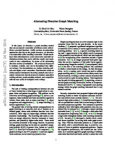
where ‖𝑥‖0 is the 𝑙0 -norm of 𝑥. Unfortunately, (103) is a combinatorial optimization problem of which the computational complexity grows exponentially with the signal size 𝑛. A key result in [17, 18] is that if 𝑥 is sparse, the sparsest solution of (103) can be obtained with overwhelming probability by solving the convex optimization problem (77). Next, we consider CS which is actually a kind of application of the BP method in complex variables. 5.1.1. The Effects of the Parameter 𝜌. We demonstrate the complex signal sampling and recovery techniques with a discrete-time complex signal 𝑥 of length 𝑛 = 300 with sparsity 𝑟 = 30 which is generated randomly. 𝐴 𝑝×𝑛 is a random sensing matrix with 𝑝 = 120. The variables 𝑢0 and 𝑧0 are initialized to be zero. We set the two tolerances of primal and dual residuals equal to 10−6 . In order to understand the effects of the parameter 𝜌 on the convergence, we set the penalty

parameter 𝜌 from 0.1 to 20 with the step 0.1. We have repeated the same experiment 100 times with the same parameter 𝜌. The average runtime, the average numbers of iterations, and the average primal and dual errors of the ADMM for the different choices of the parameter 𝜌 are presented in Figure 1. It is clear from Figure 1 (top) that when 2 ≤ 𝜌 ≤ 4, the average runtime and the average iterations are reasonable. From Figure 1 (bottom), we can observe that, with the parameter 𝜌 increasing, the primal error decreases while the dual error becomes bigger. Numerical simulations suggest that choosing 𝜌 ∈ [2, 4] could accelerate the convergence of the ADMM. 5.1.2. The Effects of Tolerances for the Primal and Dual Residuals. Now, we take the different tolerances for the primal residuals 𝜖pri and the dual residuals 𝜖dual to analyze the performance of the ADMM, where sparse 𝑟 = 0.1𝑛, measurements 𝑝 = 4𝑟, the penalty parameter 𝜌 = 2, and 𝜖pri = 𝜖dual = 𝜖. We take two different signal lengths 𝑛 = 400 and 𝑛 = 600. We have repeated the same experiment 100 times by a set of randomly generated data. For different choices of 𝜖, the average numbers of iterations and the executing time of the above ADMM algorithm (102) are presented in Table 1. It is shown that, with the increasing of precision, the number of iterations increases accordingly while increasing of executing time is not obvious. In Figure 2(a), the full line describes the changes of the primal residuals 𝑟𝑘 . In Figure 2(b), the full line describes the

Mathematical Problems in Engineering

11

Table 1: Numerical results on the different tolerances for residuals. 𝑛 400 400 400 400 400 400 400

𝜖 10−1 10−2 10−3 10−4 10−5 10−6 10−7

Iteration 21.56 37.80 55.68 78.04 119.80 139.00 161.64

𝑛 600 600 600 600 600 600 600

Time 0.0459 0.0482 0.0571 0.0603 0.0951 0.0956 0.1056

100

10−10

Iteration 23.34 40.52 59.20 92.46 114.98 149.26 230.24

Time 0.1182 0.1474 0.1720 0.2238 0.2590 0.3063 0.4346

1010 ‖sk ‖2

‖rk ‖2

1010

𝜖 10−1 10−2 10−2 10−4 10−5 10−6 10−7

0

20

40

60

80

100

120

140

160

100 10−10

0

20

40

Iteration k (a)

60

80 100 Iteration k

120

140

160

(b)

Figure 2: Norms of primal residual (a) and dual residual (b) versus iteration.

changes of the dual residuals 𝑠𝑘 . The dotted lines in Figures 2(a) and 2 (b) represent the original residual tolerance 𝜖pri = 10−6 and dual residuals tolerance 𝜖dual = 10−6 , respectively. From Figure 2, we can see that the two residuals descend monotonously.

To get the compression of sparse signal 𝑥, we can first calculate 𝑏 from 𝑏 = 𝐴𝑥. 𝐴 is a random complex matrix of size 𝑝 × 𝑛, where 𝑝 = 800, 𝑛 = 2000, and the sampling rate is 40%. Substituting 𝐴 and 𝑏 into the optimization model as presented in (77), that is, minimize

5.2. Reconstruction of Electroencephalogram Signal by Using Complex ADMM. Electroencephalogram (EEG) signal is a weak bioelectricity of brain cells group, which can be recorded by placing the available electrodes on the scalp or intracranial detect. The EEG signal could reflect the brain bioelectricity rhythmic activity regularity of random nonstationary signal. In this area, much is known for clinical diagnosis and brain function [42]. Because EEG data is large, a very meaningful work is to compress EEG data. It is to effectively reduce the amount of data at the same time and to guarantee that the main features basically remain unchanged [43, 44]. In this paper, EEG signals are recorded with a g.USBamp and a g.EEGcap (Guger Technologies, Graz, Austria) with a sensitivity of 100 V, band pass filtered between 0.1 and 30 Hz, and sampled at 256 Hz. Data are recorded and analyzed using the ECUST BCI platform software package developed through East China University of Science and Technology [45, 46]. We get the complex signal 𝑥𝑜 by performing the discrete Fourier transform (DFT) on EEG signal 𝑠; that is, 𝑥𝑜 = F(𝑠), with signal 𝑠 with length 𝑛 = 2000. Original EEG signal 𝑠 is not sparse, but its DFT signal 𝑥𝑜 becomes the approximate sparse signal; see Figure 3. The hard threshold of 𝑥𝑜 is properly set, which leads to 𝑥 with 90 percent zero valued entries, and 𝑥 is the approximation of 𝑥𝑜 .

̃ 1 : 𝐴𝑥̃ = 𝑏, 𝑥̃ ∈ 𝐶𝑛 } , {‖𝑥‖

(104)

we can obtain the sparse optimal solution 𝑥̃ by employing the ADMM algorithm (102) in Section 4, in which 𝑥̃ is a good approximation of 𝑥. By applying the inverse discrete Fourier ̃ we can get the approximation 𝑠̃ of transform (IDFT) on 𝑥, original signal 𝑠; that is, ̃ 𝑠̃ = F−1 𝑥.

(105)

The original signal 𝑠 and its reconstruction signal 𝑠̃ can be seen in Figure 4, in which (a) is the original signal 𝑠, (b) is the reconstruction signal 𝑠̃, and (c) is the comparison of them. With the comparison of (a), (b), and (c) in Figure 4, we can observe that the reconstructed signal is in good agreement with the original signal and retains the leading characteristic. The relative error 𝛿 = norm(𝑠 − 𝑠̃)/norm(𝑠) = 0.1858. Now we separate the complex signal 𝑥 into the real part 𝑥re and the imaginary part 𝑥im and then recast it into an equivalent real-valued optimization problem. We can calculate 𝑏1 from 𝑏1 = 𝐴𝑥re and 𝑏2 from 𝑏2 = 𝐴𝑥im , respectively. Here 𝐴 is a random real matrix of size 𝑝 × 𝑛, where 𝑝 = 800, 𝑛 = 2000, and the sampling rate is 40% which is similar to the one used in the complex number domain. Substitute 𝐴 and 𝑏1 , 𝑏2 into the optimization model as presented in (77); that is, 󵄩 󵄩 minimize {󵄩󵄩󵄩𝑥̃re 󵄩󵄩󵄩1 : 𝐴𝑥̃re = 𝑏1 , 𝑥̃re ∈ 𝑅𝑛 } , (106) 󵄩 󵄩 minimize {󵄩󵄩󵄩𝑥̃im 󵄩󵄩󵄩1 : 𝐴𝑥̃im = 𝑏2 , 𝑥̃im ∈ 𝑅𝑛 } .

12

Mathematical Problems in Engineering 5000

5000

100 0

0

0

−100

−5000

−5000

0

1000

2000

0

1000

2000

5000

0

0

0

−5000

−5000

0

1000

2000

1000

0

2000

50

5000

0

0

0

−50

−5000

−5000

0

1000

2000

1000

0

2000

5000

0

0

0

−50

−5000

−5000

0

1000

2000

1000

2000

0

1000

2000

0

1000

2000

0

1000

2000

0

1000

2000

5000

0

1000

2000

5000

0

2000

5000

50

40 20 0 −20 −40

1000

5000

100 −100

0

5000

0

0

−5000

−5000

0

(a) Original EEG

1000

2000

(b) Real part of DFT

(c) Imaginary part of DFT

Figure 3: Original EEG signal and its DFT signal.

40 0 −40

40 0 0

500

1000

1500

2000

−40

0

(a) Original EEG signal

500

1000

1500

2000

(b) Reconstructed EEG signal in complex number domain

40 0 −40

0

500

1000

1500

2000

(c) Comparison of original EEG signal and its reconstructed signal

Figure 4: Original EEG signal and its reconstructed signal in the complex number domain. 40 0 −40

0

500

1000

1500

2000

40 0 −40

(a) Original EEG signal

40 0 −40

0

0

500

1000

1500

2000

(b) Reconstructed EEG signal in the real number domain

500

1000

1500

2000

(c) Comparison of original EEG signal and its reconstructed signal

Figure 5: Original EEG signal and its reconstructed signal in the real number domain.

Although 𝑥̃re and 𝑥̃im can approach 𝑥re and 𝑥im , respectively, the reconstructed signal 𝑠̃ = F−1 (𝑥̃re + 𝑖𝑥̃im ) is not consistent with the original signal 𝑠; see Figure 5. The relative error 𝛿 = norm(𝑠 − 𝑠̃)/norm(𝑠) = 0.5879. It can be seen that our new ADMM proposed in this paper performs better than the classic ADMM.

6. Conclusions In this paper, the ADMM for separable convex optimization of real functions in complex variables has been studied. By using Wirtinger calculus, we have established the convergence of the algorithm, which is the generalization of

Mathematical Problems in Engineering the one obtained in real variables. Furthermore, the BP algorithm is given in the form of the ADMM, in which projection algorithm and the soft thresholding formula are generalized from the real number domain to the complex case. The simulation results demonstrate that the ADMM can quickly solve convex optimization problems in complex variables within the scopes of the signal compression and reconstruction, which is better than the results in the real number domain.

Conflict of Interests The authors declare that there is no conflict of interests regarding the publication of this paper.

Acknowledgments The authors would like to thank Dr. Shouwei Zhao and Dr. Zhongtuan Zheng for pointing out some typos and inconsistencies in an earlier version of the paper. This research was supported by Shanghai Natural Science Fund Project (no. 14ZR1418900), the National Natural Science Foundation of China (no. 11471211), and the Scientific Research Foundation for the Returned Overseas Chinese Scholars, State Education Ministry.

References [1] M. R. Hestenes, “Multiplier and gradient methods,” Journal of Optimization Theory and Applications, vol. 4, no. 5, pp. 303–320, 1969. [2] S. Boyd, N. Parikh, E. Chu, B. Peleato, and J. Eckstein, “Distributed optimization and statistical learning via the alternating direction method of multipliers,” Foundations and Trends in Machine Learning, vol. 3, no. 1, pp. 1–122, 2011. [3] M. K. Ng, P. Weiss, and X. M. Yuan, “Solving constrained total-variation image restoration and reconstruction problems via alternating direction methods,” SIAM Journal on Scientific Computing, vol. 32, no. 5, pp. 2710–2736, 2010. [4] K. Scheinberg, S. Q. Ma, and D. Goldfarb, “Sparse inverse covariance selection via alternating linearization methods,” in Proceedings of the Annual Conference on Neural Information Processing Systems (NIPS ’10), Vancouver, Canada, December 2010. [5] R. D. C. Monteiro and B. F. Svaiter, “Implementation of a blockdecomposition algorithm for solving large-scale conic semidefinite programming problems,” Computational Optimization and Applications, vol. 57, no. 1, pp. 45–69, 2014. [6] B. S. He and X. M. Yuan, “On the 𝑂(1/𝑛) convergence rate of the Douglas-Rachford alternating direction method,” SIAM Journal on Numerical Analysis, vol. 50, no. 2, pp. 700–709, 2012. [7] M. Tao and X. M. Yuan, “On the O(1/t) convergence rate of alternating direction method with logarithmic quadratic proximal regularization,” SIAM Journal on Optimization, vol. 22, no. 4, pp. 1431–1448, 2012. [8] C. H. Chen, B. S. He, Y. Ye, and X. M. Yuan, “The direct extension of ADMM for multi-block convex minimization problems is not necessarily convergent,” Mathematical Programming, 2015.

13 [9] M. Li, X. Li, and X. M. Yuan, “Convergence analysis of the generalized alternating direction method of multipliers with logarithmic-quadratic proximal regularization,” Journal of Optimization Theory and Applications, vol. 164, no. 1, pp. 218– 233, 2015. [10] C. H. Chen, M. Li, and X. M. Yuan, “Further study on the convergence rate of alternating direction method of multipliers with logarithmic-quadratic proximal regularization,” Journal of Optimization Theory and Applications, vol. 166, no. 3, pp. 906– 929, 2015. [11] D. Gabay and B. Mercier, “A dual algorithm for the solution of nonlinear variational problems via finite element approximation,” Computers and Mathematics with Applications, vol. 2, no. 1, pp. 17–40, 1976. [12] J. Eckstein and D. P. Bertsekas, “On the Douglas-Rachford splitting method and the proximal point algorithm for maximal monotone operators,” Mathematical Programming, vol. 55, no. 1–3, pp. 293–318, 1992. [13] R. T. Rockafellar, “Augmented Lagrangians and applications of the proximal point algorithm in convex programming,” Mathematics of Operations Research, vol. 1, no. 2, pp. 97–116, 1976. [14] Y. Bai and K. Shen, “Alternating direction method of multipliers for ℓ1 -ℓ2 -regularized logistic regression model,” Journal of the Operations Research Society of China, pp. 1–11, 2015. [15] T. Y. Lin, S. Q. Ma, and S. Z. Zhang, “On the sublinear convergence rate of multi-block ADMM,” Journal of the Operations Research Society of China, vol. 3, no. 3, pp. 251–274, 2015. [16] S. Q. Ma, “Alternating direction method of multipliers for sparse principal component analysis,” Journal of the Operations Research Society of China, vol. 1, no. 2, pp. 253–274, 2013. [17] E. J. Cand`es, J. Romberg, and T. Tao, “Robust uncertainty principles: exact signal reconstruction from highly incomplete frequency information,” IEEE Transactions on Information Theory, vol. 52, no. 2, pp. 489–509, 2006. [18] D. L. Donoho, “Compressed sensing,” IEEE Transactions on Information Theory, vol. 52, no. 4, pp. 1289–1306, 2006. [19] H. Jung, K. Sung, K. S. Nayak, E. Y. Kim, and J. C. Ye, “Kt FOCUSS: a general compressed sensing framework for high resolution dynamic MRI,” Magnetic Resonance in Medicine, vol. 61, no. 1, pp. 103–116, 2009. [20] M. Lustig, D. Donoho, and J. M. Pauly, “Sparse MRI: the application of compressed sensing for rapid MR imaging,” Magnetic Resonance in Medicine, vol. 58, no. 6, pp. 1182–1195, 2007. [21] M. A. Herman and T. Strohmer, “High-resolution radar via compressed sensing,” IEEE Transactions on Signal Processing, vol. 57, no. 6, pp. 2275–2284, 2009. [22] S. S. Chen, D. L. Donoho, and M. A. Saunders, “Atomic decomposition by basis pursuit,” SIAM Journal on Scientific Computing, vol. 20, no. 1, pp. 33–61, 1998. [23] K. C. Kwak and W. Pedrycz, “Face recognition using an enhanced independent component analysis approach,” IEEE Transactions on Neural Networks, vol. 18, no. 2, pp. 530–541, 2007. [24] V. D. Calhoun and T. Adali, “Unmixing fMRI with independent component analysis,” IEEE Engineering in Medicine and Biology Magazine, vol. 25, no. 2, pp. 79–90, 2006. [25] J. Annem¨uller, T. J. Sejnowski, and S. Makeig, “Complex spectral domain independent component analysis of electrocephalographic data,” in Proceedings of the 4th International Symposium

14

[26]

[27] [28]

[29]

[30]

[31]

[32]

[33]

[34]

[35]

[36]

[37] [38] [39] [40]

[41] [42]

[43]

[44]

Mathematical Problems in Engineering on Independent Component Analysis and Blind Signal Separation (ICA ’03), Nara, Japan, April 2003. C. N. K. Mooers, “A technique for the cross spectrum analysis of pairs of complex-valued time series, with emphasis on properties of polarized components and rotational invariants,” Deep-Sea Research and Oceanographic Abstracts, vol. 20, no. 12, pp. 1129–1141, 1973. G. Taub¨ock, “Complex noise analysis of DMT,” IEEE Transactions on Signal Processing, vol. 55, no. 12, pp. 5739–5754, 2007. L. Sorber, M. V. Barel, and L. D. Lathauwer, “Unconstrained optimization of real functions in complex variables,” SIAM Journal on Optimization, vol. 22, no. 3, pp. 879–898, 2012. J. F. Sturm, “Using SeDuMi 1.02, a Matlab toolbox for optimization over symmetric cones,” Optimization Methods and Software, vol. 11/12, no. 1–4, pp. 625–653, 1999. K. C. Toh, M. J. Todd, and R. H. T¨ut¨unc¨u, “SDPT3—a MATLAB software package for semidefinite programming, version 1.3,” Optimization Methods and Software, vol. 11/12, no. 1–4, pp. 545– 581, 1999. J. L¨ofberg, “YALMIP: a toolbox for modeling and optimization in MATLAB,” in Proceedings of the IEEE International Symposium on Computer Aided Control Systems Design, pp. 284–289, IEEE, Taipei, Taiwan, September 2004. B. Jiang, S. Q. Ma, and S. Z. Zhang, “Alternating direction method of multipliers for real and complex polynomial optimization models,” Optimization, vol. 63, no. 6, pp. 883–898, 2014. W. Wirtinger, “Zur formalen Theorie der Funktionen von mehr komplexen Ver¨anderlichen,” Mathematische Annalen, vol. 97, no. 1, pp. 357–375, 1927. P. J. Schreier and L. L. Scharf, Statistical Signal Processing of Complex-Valued Data: The Theory of Improper and Noncircular Signals, Cambridge University Press, Cambridge, UK, 2010. T. Adali, P. J. Schreier, and L. L. Scharf, “Complex-valued signal processing: the proper way to deal with impropriety,” IEEE Transactions on Signal Processing, vol. 59, no. 11, pp. 5101–5125, 2011. D. H. Brandwood, “A complex gradient operator and its application in adaptive array theory,” IEE Proceedings H: Microwaves, Optics and Antennas, vol. 130, no. 1, pp. 11–16, 1983. H. Groemer, “On an inequality of Minkowski for mixed volumes,” Geometriae Dedicata, vol. 33, no. 1, pp. 117–122, 1990. S. Boyd and L. Vandenberghe, Convex Optimization, Cambridge University Press, Cambridge, UK, 2004. D. Zhang, The p-perfectly convex set and absolutely p-persectly convex set [M.S. thesis], Shanghai University, 2010, (Chinese). P. L. Combettes and J. C. Pesquet, “Proximal splitting methods in signal processing,” in Fixed-Point Algorithms for Inverse Problems in Science and Engineering, vol. 49, pp. 185–212, Springer, Berlin, Germany, 2011. G. R. Wang, Y. Wei, and S. Z. Qiao, Generalized Inverses: Theory and Computations, Science Press, Beijing, China, 2003. ¨ E. D. Ubeyli and ˙I. G¨uler, “Features extracted by eigenvector methods for detecting variability of EEG signals,” Pattern Recognition Letters, vol. 28, no. 5, pp. 592–603, 2007. Z. Zhang and B. D. Rao, “Sparse signal recovery with temporally correlated source vectors using sparse Bayesian learning,” IEEE Journal on Selected Topics in Signal Processing, vol. 5, no. 5, pp. 912–926, 2011. Z. Zhang and B. D. Rao, “Extension of SBL algorithms for the recovery of block sparse signals with intra-block correlation,”

IEEE Transactions on Signal Processing, vol. 61, no. 8, pp. 2009– 2015, 2013. [45] J. Jin, B. Z. Allison, Y. Zhang, X. Y. Wang, and A. Cichocki, “An Erp-based BCI using an oddball paradigm with different faces and reduced errors in critical functions,” International Journal of Neural Systems, vol. 24, no. 8, Article ID 1450027, 14 pages, 2014. [46] J. Jin, I. Daly, Y. Zhang, X. Y. Wang, and A. Cichocki, “An optimized ERP brain-computer interface based on facial expression changes,” Journal of Neural Engineering, vol. 11, no. 3, Article ID 036004, 11 pages, 2014.

Advances in

Operations Research Hindawi Publishing Corporation http://www.hindawi.com

Volume 2014

Advances in

Decision Sciences Hindawi Publishing Corporation http://www.hindawi.com

Volume 2014

Journal of

Applied Mathematics

Algebra

Hindawi Publishing Corporation http://www.hindawi.com

Hindawi Publishing Corporation http://www.hindawi.com

Volume 2014

Journal of

Probability and Statistics Volume 2014

The Scientific World Journal Hindawi Publishing Corporation http://www.hindawi.com

Hindawi Publishing Corporation http://www.hindawi.com

Volume 2014

International Journal of

Differential Equations Hindawi Publishing Corporation http://www.hindawi.com

Volume 2014

Volume 2014

Submit your manuscripts at http://www.hindawi.com International Journal of

Advances in

Combinatorics Hindawi Publishing Corporation http://www.hindawi.com

Mathematical Physics Hindawi Publishing Corporation http://www.hindawi.com

Volume 2014

Journal of

Complex Analysis Hindawi Publishing Corporation http://www.hindawi.com

Volume 2014

International Journal of Mathematics and Mathematical Sciences

Mathematical Problems in Engineering

Journal of

Mathematics Hindawi Publishing Corporation http://www.hindawi.com

Volume 2014

Hindawi Publishing Corporation http://www.hindawi.com

Volume 2014

Volume 2014

Hindawi Publishing Corporation http://www.hindawi.com

Volume 2014

Discrete Mathematics

Journal of

Volume 2014

Hindawi Publishing Corporation http://www.hindawi.com

Discrete Dynamics in Nature and Society

Journal of

Function Spaces Hindawi Publishing Corporation http://www.hindawi.com

Abstract and Applied Analysis

Volume 2014

Hindawi Publishing Corporation http://www.hindawi.com

Volume 2014

Hindawi Publishing Corporation http://www.hindawi.com

Volume 2014

International Journal of

Journal of

Stochastic Analysis

Optimization

Hindawi Publishing Corporation http://www.hindawi.com

Hindawi Publishing Corporation http://www.hindawi.com

Volume 2014

Volume 2014