Extension of linear-scaling divide-and-conquer-based correlation method to coupled cluster theory with singles and doubles excitations
Masato Kobayashi1,2 and Hiromi Nakai1,a)
1
Department of Chemistry and Biochemistry, School of Advanced Science and
Engineering, Waseda University, Tokyo 169-8555, Japan 2
Department of Theoretical and Computational Molecular Science, Institute for
Molecular Science, Okazaki 444-8585, Japan
a)
Electronic mail:
[email protected]
-1-
(ABSTRACT) This paper describes the extension of the linear-scaling divide-and-conquer (DC)-based correlation method to the coupled cluster with singles and doubles excitations (CCSD) theory. In this DC-CCSD method, the CCSD equations are solved for all subsystems including their buffer regions with the use of the subsystem orbitals, which are obtained by the DC-Hartree-Fock method. Then, the correlation energy of the total system is evaluated by summing up the subsystem contributions other than the buffer regions by the energy density analysis technique. Numerical applications demonstrate that the present DC-CCSD gives highly accurate results with drastically less computational costs with regard to the required computer memory, scratch-disk capacity, and calculation time.
-2-
I. INTRODUCTION
In the field of computer science, the divide-and-conquer (DC) method first appeared in the early 1960s in the form of the Karatsuba multiplication algorithm.1 In the Karatsuba algorithm, the computational cost for multiplying two n-digit numbers is reduced from O ( n 2 ) to O ( n log 3 ) by representing the original numbers by two-digit 2
numbers in base b, i.e., x x1b x 2 , and recursively calling this procedure. Since then, various types of algorithms based on the DC philosophy have been proposed. In these algorithms, a complicated problem is divided into two or more smaller problems and the solutions of the smaller problems are combined to obtain the solution of the original problem. Some examples of such algorithms are sorting algorithms such as merge sort and quicksort, search algorithms like binary search, and fast Fourier transformation (for details on these algorithms, see Ref. 2, for example). In the field of quantum chemistry, Yang and coworkers3,4 first imported this DC philosophy into the non-iterative density functional theory (DFT) for enabling linear-scaling computation with respect to the system size. In the density-matrix-based DC formalism,4 the density matrix of the total system is represented as the sum of subsystem contributions, which are constructed from Fock matrices corresponding to
-3-
the subsystems. Recently, Akama et al.5,6 assessed the performance of Yang’s DC method when applied to the Hartree-Fock (HF) procedure, that is, DC-HF. Because the effect from the environment of the subsystem can be taken into account by the so-called buffer region, the DC method can provide reliable results by adopting a moderate-size buffer region. It is noted that the DC-HF method is capable of accurately dealing with delocalized systems such as polyene chains, which have been challenging targets for various linear-scaling techniques. Two strategies have been proposed for evaluating the second-order Møller-Plesset (MP2) correlation energy based on the DC-HF calculations. After a DC-HF calculation, the density matrix of the total system and molecular orbitals corresponding to subsystems can be obtained. The first DC-HF-based MP2 strategy, which is termed DC-DM MP2,7 applies the DC-HF density matrix to the DM-Laplace MP2 method.8–10 As in the case of the original Laplace MP2 methods,10–15 the DC-DM MP2 method is categorized into a domain-free approach, where the performance is considerably dependent on the threshold screening. In other words, the procedure of the DC-DM MP2 method for obtaining the correlation energy does not divide the total problem into smaller problems, i.e., it is not based on the original DC philosophy. The alternative method, which is termed DC-MP2,16 evaluates the correlation
-4-
energies of all subsystems by using DC subsystem orbitals and combines these energies. This procedure for obtaining the correlation energy is clearly based on the DC philosophy. Note that the energy density analysis (EDA) scheme17 plays an important role to estimate the correlation energies of subsystems other than their buffer regions. Numerical tests have confirmed the linear-scaling behavior of the DC-MP2 calculations. In the previous paper proposing the DC-MP2 method,16 we presented the general formula (Eqs. (20) and (21) in Ref. 16) to evaluate the correlation energy based on the DC method. We here implemented the DC-based coupled-cluster with singles and doubles (DC-CCSD) code and numerically assessed this method from the viewpoints of accuracy and computational cost. The DC-CCSD method differs from previous local CCSD methods18–25 in that subsystem orbitals obtained by the DC-HF calculations are used instead of localized orbitals or atomic orbitals. Furthermore, unlike with several low-scaling CCSD methods,26–29 intersubsystem contributions do not appear explicitly in DC-CCSD but are incorporated into subsystem contributions. The organization of this paper is as follows. In Section II, we describe the theoretical aspects of DC-CCSD, which involve brief explanations of DC-HF, EDA for correlation energy, and dual-buffer DC-based correlation scheme. Section III shows the
-5-
numerical applications of the DC-CCSD method to polyene chains. Concluding remarks are given in Section IV.
-6-
II. THEORETICAL ASPECTS A. Divide-and-conquer Hartree-Fock (DC-HF) method
The DC-based correlation method utilizes the subsystem orbitals obtained from the DC-HF calculation. Since the detailed procedure of the DC-HF method is explained well in some preceding articles,5,6 we here summarize its essence. In the DC-HF method, the density matrix of the total system, D, is constructed of subsystem contributions as follows: DC . D D D
(1)
D represents the local density matrix for subsystem , which is expanded by
subsystem bases . Subsystem bases consist of two types of AOs, that is, central AOs (S()) and environmental AOs (B()) that belong to the subsystem itself (usually called the “central region”) and its neighboring region (called the “buffer region”), respectively. The union of the central and buffer regions is called the “localization region.” D is obtained by using the Fermi level F and Fermi function f ( x ) [1 exp( x )]1 with an inverse temperature parameter as follows: * D p f ( F i )C i C i .
(2)
i
where p is the partition matrix with elements
-7-
p
and
for S ( ) and S ( )
1 1 / 2 0
C
and
i
for ( S ( ) and B ( )) or ( B ( ) and S ( )) ,
(3)
for S ( ) and S ( )
i
represent the orbital coefficients and orbital energies for
subsystem ; they are the solutions of the following local eigen-problem in subsystem
: F C i i S C i .
(4)
Here, S and F represent local overlap and Fock matrices in the subsystem bases
, respectively. The Fermi level,
F , can be determined by the constraint of the
total number of electrons, ne: ne
(D
S ) .
(5)
Then, the density matrix of the total system can be obtained from Eq. (1).
B. Energy density analysis for correlation energy
The DC-based correlation method16 adopts the subsystem orbitals, which are constructed in the localization region, containing not only the central region but also the buffer region. While the buffer regions overlap in several subsystems, the central ones have no overlap. To avoid double counting, the correlation energies only in the
-8-
central regions should be estimated. Thus, we adopted the EDA technique,17 which originally partitions the total energy into atomic contributions by analogy to Mulliken population analysis.30 The electron correlation energy of the closed-shell system can be expressed in terms of active occupied orbitals i , j and virtual orbitals a , b with the two-electron
integral
notation
ij ab
* i
1
(r1 ) j (r2 ) r12 a (r1 ) b (r2 ) d r1d r2 *
as
follows:31 E corr
occ vir
ij
~ ~ ij ab 2 tij ,ab tij ,ba .
(6)
ab
~ where tij ,ab represents an effective two-electron excitation coefficient. In MP2 theory, ~ tij ,ab is given by
~ tij ,ab
ab ij
a b i j
(7)
,
~ where i represents the energy of orbital i . For the CCSD method, tij ,ab is given
by ~ tij ,ab t i ,a t j ,b t i ,b t j ,a t ij ,ab ,
(8)
where t i ,a and t ij ,ab are the so-called T1 and T2 amplitudes. To divide the correlation energy into atomic contributions, the last integral-transformation is left undone, in the same manner as that in the original EDA. Then, the correlation energy can be rewritten A using atomic correlation energies E corr as follows:
-9-
E co rr
ij
o cc v ir
~ ~ ij ab 2 tij ,a b tij ,b a
ab
o cc v ir * wo cc C i j ab w v ir Ca ij b A A A ij a b
ato m
~ 2 tij ,a b ~ tij ,b a
ato m
E
,
A co rr
(9)
A
A E corr
occ vir
w C ij
ab
*
occ
A
i
~ ~ j ab w vir C a ij b 2 tij ,ab tij ,ba , A
(10)
where wocc and wvir are parameters constrained by wocc wvir 1 , and they represent the weights of occupied and virtual contributions, respectively.
C. Divide-and-conquer (DC)-based correlation method
In the DC-based correlation method, the total correlation energy of a certain system is evaluated by summing up the correlation energies corresponding to the central regions of individual subsystems: subsystem
E corr
E
corr
.
(11)
Here, the correlation energy of subsystem , E corr , is evaluated by means of DC-HF
orbitals as follows: E corr
occ( ) vir( )
ij
ab
wocc C i* j a b w vir Ca i j b S ( ) S ( )
~ 2 tij ,ab ~ tij,ba
,
(12)
- 10 -
where i and j represent occupied subsystem orbitals that have orbital energies i and j less than the Fermi level F that is determined in the DC-HF calculation,
and a and b represent virtual subsystem orbitals with orbital energies a and ~ b greater than F . tij,ab is the effective two-electron excitation amplitude for
subsystem , and it is defined by ~ tij ,ab t i,a t j ,b t i,b t j ,a tij,ab ,
(13)
where t i,a and t ij,ab are T1 and T2 amplitudes, which are determined by solving the CCSD equation for subsystem . Note that there is no double counting of correlation energy in Eq. (12) although three MOs in integrals as well as effective amplitudes still contain contributions from the buffer region. They are used only for incorporating the effect of environment into the correlation energy of the central region (pay attention to Eq. (9) where only one MO is decomposed into AOs but the right-hand side of the equation still keeps the total correlation energy). In the previous article,16 we assessed the weight parameters of wocc and wvir in the DC-MP2 method and clarified that the results by (wocc, wvir) = (1, 0) commonly evaluate correlation energies more accurately than those by (wocc, wvir) = (0, 1). Thus, the reduced energy expression of Eq. (12), E corr
occ( ) vir( )
C
i j
a b S ( )
* i
j a b 2 tij,ab tij,ba , ~
- 11 -
~
(14)
is employed in this article.
D. Dual-buffer DC-based correlation method
In the present calculations, we utilized the dual-buffer DC-based correlation scheme as described below. The dual-buffer treatment is expected to further reduce the computational cost of the DC-based correlation method by adopting a smaller buffer region for correlation calculations than for the HF calculation. The procedure of the dual-buffer treatment is as follows: 1. Solve the DC-HF equation (or the conventional HF equation) with large buffer regions until convergence in order to obtain the converged total Fock matrix and HF energy E DC HF (or E HF ). 2. Once solve the DC-HF equation with smaller buffer regions in order to obtain subsystem orbitals and orbital energies. The Fermi level F that separates occupied and virtual orbitals used in the correlation calculation is also determined from the constraint of Eq. (5). 3. Perform the correlation calculation by using the subsystem orbitals and orbital energies determined at Step 2 and obtain CCSD energies corresponding to the
- 12 -
localization regions, E CCSD .
4. Evaluate the subsystem correlation energies corresponding to the central regions, E DCCCSD , by the EDA technique and sum up the subsystem
correlation energies to evaluate the total correlation energy, E DC-CCSD . 5. Sum up the HF energy, E DC HF (or E HF ) in Step 1; and the correlation energy, E DC-CCSD in Step 4; in order to obtain the total CCSD energy, E DC-CCSD .
- 13 -
III. NUMERICAL ASSESSMENTS A. Computational details
The present DC-CCSD method was assessed in the calculations of polyene chain systems, CnHn+2 (n = 10–100), by comparing the findings with the conventional CCSD results. DC-MP2 calculations were also performed for comparing the trend of correlation energy deviations. The following results were obtained by the modified version of the GAMESS program:32 namely, our DC-HF code was merged and the original CCSD code by Piecuch et al.33 was modified. In DC-HF calculations, the inverse temperature parameter of the Fermi function, was set to 125.0 a.u., which corresponds to 2526 K. All the following calculations were performed with the 6-31G basis set.34 Basis-set dependences for the DC-HF and DC-MP2 calculations have been investigated in our previous studies,5,16 which have clarified that the discrepancies from the conventional results exhibit no remarkable trend for several classes of basis sets. While it is possible to adopt the frozen-core (and/or frozen-virtual) orbitals in DC-CCSD calculations as well as DC-MP2, all occupied and virtual orbitals were treated as active ones except as otherwise noted. In our experience,5,6,16 both DC-HF and DC-MP2 methods can give reliable
- 14 -
results even when adopting an individual atom as the central region, which is normally a severe condition for the fragmentation techniques due to breaking of all chemical bonds. Some preliminary tests for the fragmentation showed the advantage for partitioning C2H2 (or C2H3 for the edges) units from the viewpoints of accuracy and computational cost. Thus, C2H2 (or C2H3) was adopted as a central region and several adjacent C2H2 units were treated as buffer regions. In particular, the left and right buffer regions in the DC-HF calculations were fixed at C n H n HF b
HF b
(or C n H n HF b
HF b 1
)
( nbHF 12 ), which gave mHartree-order accuracy as shown later. On the other hand, the buffer regions in the DC-CCSD calculations as well as in the DC-MP2 ones are varied as C n H n co rr b
co rr b
(or C n H n co rr b
co rr 1 b
) ( n bcorr = 2, 4, 6, and 8). Figure 1 shows a schematic
illustration for the central and buffer regions in the dual-buffer DC-CCSD calculations of C20H22. The total number of subsystems is 10. The HF and correlation buffer regions are indicated by gray and shaded areas, respectively. This figure corresponds to ( nbHF , nbcorr ) (12 , 4) .
B. Procedure and results of dual-buffer DC-CCSD
Table I shows the dual-buffer DC-CCSD results for C20H22 with the condition
- 15 -
( nbHF , nbcorr ) (12 , 4) , according to the procedure described in Section II-D. Note that all
data for the subsystems are symmetric, reflecting the molecular symmetry: i.e., subsystem pairs (1, 10), (2, 9), (3, 8), (4, 7), and (5, 6). For comparison, the HF and CCSD energies obtained by the conventional procedure are listed in the bottom line. There is no need to compute the energy values given in brackets in a typical procedure. Step 1 gives the HF energy of the total system. The energies corresponding to the subsystems were estimated by the subsystem energy technique presented in the previous paper.5 No energy data are given at Step 2, which only calculates the orbitals and orbital energies for the CCSD calculations in the next step. Step 3 evaluates the CCSD correlation energies for individual subsystems involving buffer regions as well as central regions. The absolute value of the correlation energies, ECCSD , increases
with respect to the size of the localization regions, namely, C6H7, C8H9, C10H10, and C10H11 for = (1, 10), (2, 9), (4, 5, 6, 7), and (3, 8), respectively. The sum
E
CCSD
remarkably overestimates the correlation energy of the total system, due
to the double counting of buffer regions. The EDA technique extracts the correlation energies for the central regions, E DCCCSD . The summation
E
DC - CCSD
is
sufficiently close to the conventional value. A similar agreement is seen for the total energy in Step 5.
- 16 -
C. Correlation buffer-size dependence
Next, we examine the correlation buffer-size ( n bcorr ) dependence in the DC-CCSD calculation of C20H22 by fixing nbHF 12 . Table II shows the computational size by changing n bcorr = 2, 4, 6, and 8, i.e., the maximum number of occupied and virtual orbitals, Nocc and Nvir, respectively; the maximum number of CCSD amplitudes, Namp; required memory in MB; and scratch-disk capacity in GB for CCSD calculations of the subsystems. Namp for the determinant-based treatment is estimated by using Nocc and Nvir as follows: 2 2 N amp N occ N vir N occ N vir ,
(15)
Here, the first and second terms on the right-hand side correspond to the number of T1 and T2 amplitudes, respectively. While the number of T2 amplitudes can be reduced by means of the index permutation symmetries, its order is unchanged, that is, O(n4). For Namp, the required memory, and the scratch-disk capacity, the ratios with respect to the conventional CCSD values are shown in parentheses. In the DC-CCSD approach, Namp as well as memory and disk sizes increase with the correlation buffer size, n bcorr . The ratios for the required memory shown in parentheses agree with those for Namp, i.e., the
- 17 -
required memory is proportional to Namp. It is noted that in principle, the DC-CCSD calculations require approximately equal computational size (i.e., memory and disk sizes) for different lengths of polyene chains, only if the same buffer size, n bcorr , is adopted. This is because the largest subsystem size is conserved for identical n bcorr . On the other hand, the computational size of the conventional CCSD calculation increases quasi-linearly with respect to the number of amplitudes; thus, it is roughly estimated as O(n4). Table III compares the correlation energies of C20H22 calculated by the DC-CCSD method with several buffer sizes, i.e., n bcorr = 2, 4, 6, and 8. The computational conditions are the same as the case in Table II. The results for the DC-MP2 calculations are also tabulated. The correlation energies obtained by the conventional CCSD and MP2 methods are listed in the bottom line. Energy deviations from the conventional results are shown in parentheses and plotted with respect to the correlation buffer size, n bcorr , in Fig. 2. Both DC-CCSD and DC-MP2 errors seem to decrease with oscillation as the buffer size increases. The errors for nbcorr 4 are less than 1 mHartree, namely, chemical accuracy. Note that the DC-CCSD and DC-MP2 errors are of the same order of magnitude.
- 18 -
D. System-size dependence
Next, we assessed the system-size dependence of the accuracy of the DC-CCSD method. Table IV compares the results of DC and conventional CCSD for polyene chain systems, CnHn+2 (n = 10, 12, 14, 16, 20, 30, 40, 50, 60, and 100). HF and correlation buffer sizes are fixed at ( nbHF , nbcorr ) (12 , 4) . Conventional CCSD results are given for n 20 with the limitation in our computational resources, that is, the memory-size limit is 16 GB. Energy deviations from the conventional results are shown in parentheses. The HF energy is evaluated by using the approximate total density matrix obtained from the DC-HF procedure. The DC-HF errors for n 14 become approximately zero because the full Fock matrix is used for the calculations of all subsystems due to nbHF 12 . It is notable that even for using the full Fock matrix, the DC-HF calculation involves an approximation in adopting the Fermi function with a finite temperature. For n 16 , the DC-HF error quasi-linearly increases with the system size. The correlation-energy error monotonically decreases with an increase in n. The errors in the DC-CCSD energies, EDC-CCSD, are less than 0.12 mHartree. In Table V, we show the system-size dependence of the CPU time. Figure 3 plots the CPU times for DC and conventional CCSD calculations of polyene chains, CnHn+2
- 19 -
(n = 10–100). The times for the HF procedure are not included. We adopted the same buffer size as that in the case for Table IV. An Intel Xeon X5355 (2.66 GHz) processor was used on a single core. The CPU times of the DC-CCSD calculations reduced drastically from those in the conventional CCSD, except in the case of a considerably small system (n = 10). According to the scaling analysis, the CPU time of the present DC-CCSD method scales with O(n1.4), in contrast to O(n5.7) for the conventional CCSD. We can conclude that the DC-CCSD method must be a real breakthrough as a practical technique to perform accurate quantum chemical calculations of large systems such as biomolecules and functional nanomaterials.
E. Inhomogeneous System
In DC-CCSD method, the calculation of a homogeneous system such as a polyene chain might seem to be an easy case. Thus, we performed the DC-CCSD calculation of an inhomogeneous system C19NH20F (Fig. 4), where one hydrogen atom and one CH group in the C20H22 polyene chain are substituted with fluorine and nitrogen atoms, respectively. Central and buffer regions were defined in the same manner as the homogeneous polyene chain. HF and correlation buffer sizes are fixed at
- 20 -
( nbHF , nbcorr ) (12 , 4) . The frozen-core approximation is adopted in this calculation.
Table VI shows the DC-CCSD subsystem energies for C19NH20F together with the HF and CCSD energies obtained by the conventional procedure listed in the bottom line. To clarify the inhomogeneity of the system, the DC-HF Mulliken charges of the subsystems are also listed in the table. There is no need to compute the energy values given in brackets in a typical procedure. The energy deviations from the conventional results are shown in parentheses. Although the subsystem energies vary greatly depending on the site of subsystems as compared to the homogeneous system shown in Table I, the deviation of the total energy is negligibly small, namely, ~0.2 mHartree. Therefore, the DC-CCSD scheme is greatly expected to work well not only for uniform systems but also for inhomogeneous ones.
- 21 -
IV. CONCLUDING REMARKS
In this study, we extended the DC-based correlation method, which combines the DC method of Yang3,4 with EDA of Nakai,17 to the CCSD theory. The present method, which is called DC-CCSD, only requires effort for solving the CCSD equations of subsystems. In the DC-CCSD method, the required computational resources are dependent on the size of the buffer region. Further reduction in the computational cost was achieved by the dual-buffer DC-based correlation technique, which applies two different sizes of buffer region for HF and correlation calculations. The DC-CCSD method gives accurate CCSD energy for a comparatively small buffer region. Note that the computational size is less dependent on the size of the total system and that the CPU time is scaled quasi-linearly with respect to the system size. Although the present results are promising for enabling accurate large-scale quantum chemical calculations, we are still facing a big problem: the enormous computational cost of the CCSD calculation even in a localization region of the DC method. One possible solution for this problem is the parallelization of the CCSD calculation of a subsystem.35–38 Integral reducing techniques such as the resolution of the identity39 are also possible solutions.
- 22 -
In addition, there are some hopeful extensions of the present method. The most desired one would be the energy gradient method. We have implemented the energy gradient code for DC-HF and DFT calculations40 in the same procedure by Yang and coworkers.4,41 The geometry optimization using this analytical energy gradient works reasonably well, although its accuracy depends on the size of the buffer region. However, due to the demands of the derivatives of MO coefficients and CCSD amplitudes in the analytical energy gradient of CCSD, some refinement seems to be needed for achieving the linear-scaling computation. In addition, the extension to the treatment of perturbative triples excitations (e.g., CCSD[T]42 and CCSD(T)43) and its improved scheme by Piecuch and coworkers for treating bond breaking (renormalized and completely renormalized CCSD(T)44) is also desirable. Furthermore, it is interesting to apply the present method to extended systems. The combination of the present method with the periodic CCSD formalism by Hirata et al.45,46 will enable accurate ab initio treatment of these systems.
- 23 -
ACKNOWLEDGMENTS
Some of the present calculations were performed at the Research Center for Computational Science (RCCS), Okazaki Research Facilities, National Institutes of Natural Sciences (NINS). This study was supported in part by a Grant-in-Aid for Scientific Research on Priority Areas “Molecular Theory for Real Systems” KAKENHI 18066016 from the Ministry of Education, Culture, Sports, Science and Technology (MEXT), Japan; by the Nanoscience Program in the Next Generation Super Computing Project of the MEXT; by the Global Center Of Excellence (COE) “Practical Chemical Wisdom” from the MEXT; and by a project research grant for “Development of high-performance computational environment for quantum chemical calculation and its assessment” from the Research Institute for Science and Engineering (RISE), Waseda University. One of the authors (MK) is grateful for a Research Fellowship for Young Scientists from the Japan Society for the Promotion of Science (JSPS).
- 24 -
(References) 1
A. Karatsuba and Yu. Ofman, Sov. Phys. Dokl. 7, 595 (1963).
2
W. H. Press, S. A. Teukolsky, W. T. Vetterling, and B. P. Flannery, Numerical Recipes in Fortran 77, second edition (Cambridge University Press, Cambridge, England, 1992).
3
W. Yang, Phys. Rev. Lett. 66, 1438 (1991).
4
W. Yang and T.-S. Lee, J. Chem. Phys. 103, 5674 (1995).
5
T. Akama, M. Kobayashi, and H. Nakai, J. Comput. Chem. 28, 2003 (2007).
6
T. Akama, A. Fujii, M. Kobayashi, and H. Nakai, Mol. Phys. 105, 2799 (2007).
7
M. Kobayashi, T. Akama, and H. Nakai, J. Chem. Phys. 125, 204106 (2006).
8
P. R. Surján, Chem. Phys. Lett. 406, 318 (2005).
9
M. Kobayashi and H. Nakai, Chem. Phys. Lett. 420, 250 (2006).
10
P. Y. Ayala and G. E. Scuseria, J. Chem. Phys. 110, 3660 (1999).
11
J. Almlöf, Chem. Phys. Lett. 181, 319 (1991).
12
M. Häser and J. Almlöf, J. Chem. Phys. 96, 489 (1992).
13
M. Häser, Theor. Chim. Acta 87, 147 (1993).
14
G. Rauhut and P. Pulay, Chem. Phys. Lett. 223, 248 (1996).
15
A. K. Wilson and J. Almlöf, Theor. Chim. Acta 95, 49 (1997).
- 25 -
16
M. Kobayashi, Y. Imamura, and H. Nakai, J. Chem. Phys. 127, 074103 (2007).
17
H. Nakai, Chem. Phys. Lett. 363, 73 (2002).
18
C. Hampel and H.-J. Werner, J. Chem. Phys. 104, 6286 (1996).
19
M. Schütz and H.-J. Werner, J. Chem. Phys. 114, 661 (2001).
20
M. Schütz, Phys. Chem. Chem. Phys. 4, 3941 (2002).
21
M. Schütz and F. R. Manby, Phys. Chem. Chem. Phys. 5, 3349 (2003).
22
G. E. Scuseria and P. Y. Ayala, J. Chem. Phys. 111, 8330 (1999).
23
J. E. Subotnik, A. Sodt, and M. Head-Gordon, J. Chem. Phys. 125, 074116 (2006).
24
J. E. Subotnik, A. Sodt, and M. Head-Gordon, J. Chem. Phys. 128, 034103 (2008).
25
O. Christiansen, P. Manninen, P. Jørgensen, and J. Olsen, J. Chem. Phys. 124, 084103 (2006).
26
S. Li, J. Ma, and Y. Jiang, J. Comput. Chem. 23, 237 (2002).
27
S. Li, J. Shen, W. Li, and Y. Jiang, J. Chem. Phys. 125, 074109 (2006).
28
N. Flocke and R. J. Bartlett, J. Chem. Phys. 121, 10935 (2004).
29
D. G. Fedorov and K. Kitaura, J. Chem. Phys. 123, 134103 (2005).
30
R. S. Mulliken, J. Chem. Phys. 23, 1833 (1955).
31
R. K. Nesbet, Adv. Chem. Phys. 14, 1 (1969).
32
M. W. Schmidt, K. K. Baldridge, J. A. Boatz, S. T. Elbert, M. S. Gordon, J. J.
- 26 -
Jensen, S. Koseki, N. Matsunaga, K. A. Nguyen, S. Su, T. L. Windus, M. Dupuis, and J. A. Montgomery, J. Comput. Chem. 14, 1347 (1993). 33
P. Piecuch, S. A. Kucharski, K. Kowalski, and M. Musial, Comput. Phys. Comm. 149, 71 (2002).
34
W. J. Hehre, R. Ditchfield, and J. A. Pople, J. Chem. Phys. 56, 2257 (1972).
35
A. P. Rendell, T. J. Lee, and A. Komornicki, Chem. Phys. Lett. 178, 462 (1991).
36
J. L. Bentz, R. M. Olson, M. S. Gordon, M. W. Schmidt, and R. A. Kendall, Comput. Phys. Comm. 176, 589 (2007).
37
R. M. Olson, L. B. Jonathan, R. A. Kendall, M. W. Schmidt, and M. S. Gordon, J. Chem. Theory Comput. 3, 1312 (2007).
38
T. Janowski, A. R. Ford, and P. Pulay, J. Chem. Theory Comput. 3, 1368 (2007).
39
A. P. Rendell and T. J. Lee, J. Chem. Phys. 101, 400 (1994).
40
H. Nakai, D. Sakura, A. Fujii, T. Akama, and M. Kobayashi, unpublished.
41
Q. Zhao and W. Yang, J. Chem. Phys. 102, 9598 (1995).
42
M. Urban, J. Noga, S. J. Cole, and R. J. Bartlett, J. Chem. Phys. 83, 4041 (1985).
43
K. Raghavachari, G. W. Trucks, J. A. Pople, and M. Head-Gordon, Chem. Phys. Lett. 157, 479 (1989).
44
K. Kowalski and P. Piecuch, J. Chem. Phys. 113, 18 (2001).
- 27 -
45
S. Hirata, I. Grabowski, M. Tobita, and R. J. Bartlett, Chem. Phys. Lett. 345, 475 (2001).
46
S. Hirata, R. Podeszwa, M. Tobita, and R. J. Bartlett, J. Chem. Phys. 120, 2581 (2004).
- 28 -
TABLE I. The dual-buffer DC-CCSD results for the polyene chain C20H22 with the condition ( nbHF , nbcorr ) (12 , 4) . There is no need to compute the energy values in brackets in the typical DC-CCSD procedure.
Step 1a Subsystem
a
E DC HF
Step 3
E CCSD
Step 4
E DC- CCSD
Step 5
E DCCCSD
= 1
[–77.430965]
–0.584169
–0.202285
[–77.633250]
2
[–76.859731]
–0.778422
–0.193985
[–77.053716]
3
[–76.860231]
–0.973009
–0.194289
[–77.054520]
4
[–76.860394]
–0.957759
–0.194278
[–77.054672]
5
[–76.859603]
–0.957898
–0.194125
[–77.053728]
6
[–76.859603]
–0.957898
–0.194125
[–77.053728]
7
[–76.860394]
–0.957759
–0.194278
[–77.054672]
8
[–76.860231]
–0.973009
–0.194289
[–77.054520]
9
[–76.859731]
–0.778422
–0.193985
[–77.053716]
10
[–77.430965]
–0.584169
–0.202285
[–77.633250]
[–8.502515]
–1.957923
–771.699772
–1.957863
–771.699816
Sum
–769.741849
Conv.
–769.741953
–
DC-HF energies corresponding to individual subsystems are estimated by
the subsystem energy technique in Ref. 5.
- 29 -
TABLE II. Maximum numbers of occupied and virtual orbitals, Nocc and Nvir, respectively; CCSD amplitudes, Namp; and required computer memories and scratch-disk capacities for executing DC and conventional CCSD calculations of the polyene chain C20H22 at the 6-31G level. The ratios with respect to the conventional CCSD values are shown in parentheses.
n bcorr
Subsystem Nocc
Nvir
Required memory [MB]
Namp
Scratch disk [GB]
2
C6H7
22
46
1025156
(1%)
84
(1%)
2
(1%)
4
C10H11
36
76
7488432
(6%)
607
(6%)
11
(9%)
6
C14H15
50
106
28095300
(24%)
2276
(24%)
39
(34%)
8
C18H19
64
136
75768320
(64%)
6137
(64%)
106
(91%)
conv.
C20H22
71
153
118015632
(100%)
9649 (100%)
117
(100%)
- 30 -
TABLE III. Correlation buffer-size dependence of DC-MP2 and DC-CCSD energies (in Hartree) of polyene chain C20H22 at the 6-31G level. Energy deviations from conventional MP2 and CCSD results are shown in parentheses in mHartree.
corr
nb
CCSD correlation
(diff.)
MP2 correlation
(diff.)
1
–1.936999
(+20.864)
–1.765916
(+19.685)
2
–1.957923
(–0.060)
–1.785301
(+0.300)
3
–1.957465
(+0.399)
–1.785319
(+0.282)
4
–1.957644
(+0.219)
–1.785546
(+0.055)
conv.
–1.957863
–1.785601
- 31 -
TABLE IV. DC and conventional CCSD energies (in Hartree) of polyene chains CnHn+2 at the 6-31G level with the condition ( nbHF , nbcorr ) (12 , 4) . Energy deviations from conventional CCSD results are shown in parentheses in mHartree.
DC n
Conventional
EDC-CCSD
EDC-HF
EDC-CCSD
EHF
ECCSD
ECCSD
10
–385.441748
(+0.000)
–0.986754
(+0.111)
–386.428501
(+0.111)
–385.441748
–0.986865
–386.428612
12
–462.301276
(+0.000)
–1.181942
(+0.082)
–463.483218
(+0.082)
–462.301276
–1.182024
–463.483300
14
–539.161471
(+0.000)
–1.376223
(+0.058)
–540.537695
(+0.058)
–539.161471
–1.376281
–540.537753
16
–616.021763
(+0.033)
–1.570413
(+0.032)
–617.592176
(+0.066)
–616.021796
–1.570445
–617.592242
20
–769.741849
(+0.105)
–1.957923
(–0.060)
–771.699772
(+0.045)
–769.741953
–1.957863
–771.699816
30
–1154.043159
(+0.259)
–2.929941
–1156.973100
–1154.043418
–
–
40
–1538.343708
(+0.417)
–3.901560
–1542.245268
–1538.344125
–
–
50
–1922.644502
(+0.577)
–4.873151
–1927.517654
–1922.645079
–
–
60
–2306.934697
(+0.731)
–5.844584
–2312.779282
–2306.935428
–
–
100
–3844.130003
(+1.362)
–9.730935
–3853.860938
–3844.131365
–
–
- 32 -
Table V. System-size dependence of CPU time (min) for DC and conventional CCSD calculations of polyene chains CnHn+2 at the 6-31G level with the condition HF corr ( nb , nb ) (12 , 4) . An Intel Xeon X5355 (2.66 GHz) processor was used on a single
core.
DC-CCSDa
n
Conventional CCSD
10
74.2
44.8
12
115.8
120.8
14
155.5
298.9
16
194.5
623.9
20
273.6
2361.4
30
479.5
40
681.6
50
862.1
60
1060.2
100
1983.2
Order
O(n1.4)
- 33 -
O(n5.6)
TABLE VI. The dual-buffer DC-CCSD results for the inhomogeneous chain C19NH20F with the condition ( nbHF , nbcorr ) (12 , 4) . There is no need to compute the energy values in brackets in the typical DC-CCSD procedure. Frozen-core approximation is adopted for CCSD correlation calculation.
Subsystem
a
E DC HF b
Chargea
E DC- CCSD
E DCCCSD
= 1
(C2H3)
+0.001
[–77.431147]
–0.199647
[–77.630794]
2
(C2H2)
+0.035
[–76.857062]
–0.190294
[–77.047356]
3
(C2HF)
–0.085
[–175.713475]
–0.309597
[–176.023072]
4
(C2H2)
+0.029
[–76.838600]
–0.191038
[–77.029638]
5
(C2H2)
+0.011
[–76.857280]
–0.191385
[–77.048665]
6
(C2H2)
+0.011
[–76.855388]
–0.191373
[–77.046761]
7
(C2H2)
+0.241
[–76.803828]
–0.188256
[–76.992084]
8
(CNH)
–0.313
[–92.890803]
–0.219303
[–93.110106]
9
(C2H2)
+0.046
[–76.847929]
–0.190711
[–77.038640]
10
(C2H3)
+0.026
[–77.428903]
–0.199099
[–77.628002]
Sum (diff.)
–884.524415 (+0.000100)
–2.070703 (+0.000086)
–886.595118 (+0.000186)
Conv.
–884.524515
–2.070789
–886.595303
Mulliken charge at DC-HF level.
b
DC-HF energies corresponding to individual subsystems are estimated by the
subsystem energy technique in Ref. 5.
- 34 -
Figure Captions
FIG. 1. Schematic of the central and buffer regions in the present DC calculations of polyene chains C20H22. Gray and shaded areas correspond to the HF and correlation buffer regions, respectively, for ( nbHF , nbcorr ) (12 , 4) .
FIG. 2. Correlation buffer-size dependence of deviations of MP2 and CCSD correlation energies in the DC-MP2 and DC-CCSD calculations of polyene chain C20H22 from the conventional MP2 and CCSD results at the 6-31G level.
FIG. 3. System-size dependence of CPU time (min) for DC and conventional CCSD calculations of polyene chains CnHn+2 ((a) n = 10–100; (b) n = 10–20) at the 6-31G level with the condition ( nbHF , nbcorr ) (12 , 4) . An Intel Xeon X5355 (2.66 GHz) processor was used on a single core.
FIG. 4. Structure and subsystems (central regions) of the inhomogeneous test system C19NH20F.
- 35 -
FIG. 1. Kobayashi and Nakai, The Journal of Chemical Physics.
- 36 -
FIG. 2. Kobayashi and Nakai, The Journal of Chemical Physics.
- 37 -
FIG. 3. Kobayashi and Nakai, The Journal of Chemical Physics.
- 38 -
FIG. 4. Kobayashi and Nakai, The Journal of Chemical Physics.
- 39 -