Ambulance Routing Problems with Rich Constraints and Multiple

DISSERTATION Titel der Dissertation

Ambulance Routing Problems with Rich Constraints and Multiple Objectives

Verfasserin

Mag. Sophie Parragh angestrebter akademischer Grad

Doctor of Philosophy (PhD)

Wien im Mai, 2009 Studienkennzahl lt. Studienblatt

A 094 146

Dissertationsgebiet lt. Studienblatt Management Betreuer Univ. Doz. Dr. Karl F. D¨orner

Acknowledgements First of all, I would like to thank Univ. Doz. Dr. Karl F. Doerner for introducing me to the field of dial-a-ride problems and for supervising and supporting my work on this book with numerous ideas, extensive discussions, and constructive feedback. Then, I would like to thank Prof. Dr. Richard F. Hartl for providing ideas and feedback, supporting and supervising my work, and also for granting my PhD research position (Austrian Science Fund (FWF) grant #L286-N04). Furthermore, I would like to thank a.o. Prof. Dr. Walter J. Gutjahr for directing me to the Chair for Production and Operations Management. I also wish to thank Prof. Jean-Fran¸cois Cordeau for his input and feedback during my work on Chapters 5 and 6 and for enabling my research visit at the CIRRELT in Montr´eal. Thanks are also due to my great colleagues at the Chair for Production and Operations Management. Finally, I would like to thank my family and friends, especially my parents for all their support throughout my life; and last but not least, dear Georg, thank you for your endless patience, encouragement, and support during my work on this book!

Contents List of Tables

v

List of Figures

vii

List of Algorithms

ix

1 Introduction

1

2 Summarizing the state-of-the-art

5

2.1

Introduction . . . . . . . . . . . . . . . . . . . . . . . . . . . . . . . . . . . . .

5

2.2

Classification . . . . . . . . . . . . . . . . . . . . . . . . . . . . . . . . . . . .

6

2.2.1

VRPB subclass definitions . . . . . . . . . . . . . . . . . . . . . . . . .

6

2.2.2

VRPPD subclass definitions . . . . . . . . . . . . . . . . . . . . . . . .

7

2.3

2.4

2.5

2.6

Solution methods . . . . . . . . . . . . . . . . . . . . . . . . . . . . . . . . . .

8

2.3.1

Exact methods . . . . . . . . . . . . . . . . . . . . . . . . . . . . . . .

8

2.3.2

Heuristics . . . . . . . . . . . . . . . . . . . . . . . . . . . . . . . . . . 10

2.3.3

Metaheuristics . . . . . . . . . . . . . . . . . . . . . . . . . . . . . . . 11

Solution methods for VRPB . . . . . . . . . . . . . . . . . . . . . . . . . . . . 12 2.4.1

All linehauls before backhauls (TSPCB, VRPCB) . . . . . . . . . . . 12

2.4.2

Mixed linehauls and backhauls (TSPMB, VRPMB) . . . . . . . . . . . 13

2.4.3

Divisible delivery and pickup (TSPDDP, VRPDDP) . . . . . . . . . . 14

2.4.4

Simultaneous delivery and pickup (TSPSDP, VRPSDP) . . . . . . . . 15

Solution methods for VRPPD . . . . . . . . . . . . . . . . . . . . . . . . . . . 16 2.5.1

Unpaired pickups and deliveries (PDVRP, PDTSP)

. . . . . . . . . . 16

2.5.2

Pickup and delivery problems (SPDP, PDP) . . . . . . . . . . . . . . . 17

2.5.3

Dial-a-ride problems (SDARP, DARP) . . . . . . . . . . . . . . . . . . 21

Benchmark instances . . . . . . . . . . . . . . . . . . . . . . . . . . . . . . . . 28

3 Solving a simplified problem version

31

3.1

Introduction . . . . . . . . . . . . . . . . . . . . . . . . . . . . . . . . . . . . . 31

3.2

Related Work . . . . . . . . . . . . . . . . . . . . . . . . . . . . . . . . . . . . 31

3.3

Problem definition . . . . . . . . . . . . . . . . . . . . . . . . . . . . . . . . . 33

3.4

Solution framework . . . . . . . . . . . . . . . . . . . . . . . . . . . . . . . . . 35

i

Contents

3.5

3.4.1

Pre-processing . . . . . . . . . . . . . . . . . . . . . . . . . . . . . . . 36

3.4.2 3.4.3

Initial solution . . . . . . . . . . . . . . . . . . . . . . . . . . . . . . . 36 Shaking . . . . . . . . . . . . . . . . . . . . . . . . . . . . . . . . . . . 37

3.4.4

Local search . . . . . . . . . . . . . . . . . . . . . . . . . . . . . . . . . 39

3.4.5 3.4.6

Local search frequency . . . . . . . . . . . . . . . . . . . . . . . . . . . 39 Move or not . . . . . . . . . . . . . . . . . . . . . . . . . . . . . . . . . 40

3.4.7

Solution evaluation . . . . . . . . . . . . . . . . . . . . . . . . . . . . . 40

3.4.8

Stopping criterion . . . . . . . . . . . . . . . . . . . . . . . . . . . . . 42

Computational experiments . . . . . . . . . . . . . . . . . . . . . . . . . . . . 43 3.5.1 Test instances . . . . . . . . . . . . . . . . . . . . . . . . . . . . . . . . 43 3.5.2

3.6

Comparison to tabu search on standard DARP . . . . . . . . . . . . . 44

3.5.3 Comparison to genetic algorithm with modified objective function . . 45 Summary . . . . . . . . . . . . . . . . . . . . . . . . . . . . . . . . . . . . . . 47

4 Visualizing the trade-off between costs and user inconvenience 4.1

49

Introduction . . . . . . . . . . . . . . . . . . . . . . . . . . . . . . . . . . . . . 49 4.1.1 Solution attributes in multi-objective optimization . . . . . . . . . . . 49 4.1.2

Related work . . . . . . . . . . . . . . . . . . . . . . . . . . . . . . . . 50

4.2

4.1.3 Contribution . . . . . . . . . . . . . . . . . . . . . . . . . . . . . . . . 52 Problem definition . . . . . . . . . . . . . . . . . . . . . . . . . . . . . . . . . 52

4.3

Solution framework . . . . . . . . . . . . . . . . . . . . . . . . . . . . . . . . . 54

4.4 4.5

4.6

4.3.1

Solution evaluation . . . . . . . . . . . . . . . . . . . . . . . . . . . . . 54

4.3.2 4.3.3

Request insertion . . . . . . . . . . . . . . . . . . . . . . . . . . . . . . 56 Phase one: variable neighborhood search . . . . . . . . . . . . . . . . . 56

4.3.4

Phase two: path relinking . . . . . . . . . . . . . . . . . . . . . . . . . 58

An exact method for the MO-DARP . . . . . . . . . . . . . . . . . . . . . . . 62 Computational experiments . . . . . . . . . . . . . . . . . . . . . . . . . . . . 62 4.5.1

Test instances . . . . . . . . . . . . . . . . . . . . . . . . . . . . . . . . 63

4.5.2

Quality indicators . . . . . . . . . . . . . . . . . . . . . . . . . . . . . 63

4.5.3 4.5.4

Tuning the path relinking module . . . . . . . . . . . . . . . . . . . . 65 Final results . . . . . . . . . . . . . . . . . . . . . . . . . . . . . . . . 67

Summary . . . . . . . . . . . . . . . . . . . . . . . . . . . . . . . . . . . . . . 70

5 Introducing heterogeneous patients and vehicles 73 5.1 Introduction . . . . . . . . . . . . . . . . . . . . . . . . . . . . . . . . . . . . . 73

ii

5.2

Related work . . . . . . . . . . . . . . . . . . . . . . . . . . . . . . . . . . . . 74

5.3

Problem definition . . . . . . . . . . . . . . . . . . . . . . . . . . . . . . . . . 74 5.3.1 Notation . . . . . . . . . . . . . . . . . . . . . . . . . . . . . . . . . . . 75 5.3.2

A 3-index formulation . . . . . . . . . . . . . . . . . . . . . . . . . . . 76

5.3.3

A 2-index formulation . . . . . . . . . . . . . . . . . . . . . . . . . . . 79

Contents 5.4

5.5

5.6

5.7

Valid inequalities . . . . . . . . . . . . . . . . . . . . . . . . . . . . . . . . . . 83 5.4.1

Strengthened bounds on time and load variables . . . . . . . . . . . . 83

5.4.2

Subtour elimination constraints . . . . . . . . . . . . . . . . . . . . . . 84

5.4.3

Generalized order constraints . . . . . . . . . . . . . . . . . . . . . . . 85

5.4.4

Strengthened infeasible path constraints . . . . . . . . . . . . . . . . . 86

5.4.5

Fork constraints . . . . . . . . . . . . . . . . . . . . . . . . . . . . . . 86

5.4.6

Adapted rounded capacity inequalities (only 3-index formulation) . . . 87

5.4.7

Strengthened capacity inequalities (only 3-index formulation) . . . . . 87

5.4.8

Reachability constraints (only 2-index formulation) . . . . . . . . . . . 88

Branch and cut algorithms . . . . . . . . . . . . . . . . . . . . . . . . . . . . . 88 5.5.1

The branch and cut framework . . . . . . . . . . . . . . . . . . . . . . 88

5.5.2

Pre-processing . . . . . . . . . . . . . . . . . . . . . . . . . . . . . . . 89

5.5.3

Separation heuristics . . . . . . . . . . . . . . . . . . . . . . . . . . . . 90

5.5.4

Heuristic upper bounds . . . . . . . . . . . . . . . . . . . . . . . . . . 91

Computational experiments . . . . . . . . . . . . . . . . . . . . . . . . . . . . 92 5.6.1

Test instances . . . . . . . . . . . . . . . . . . . . . . . . . . . . . . . . 92

5.6.2

Branch and cut results . . . . . . . . . . . . . . . . . . . . . . . . . . . 93

5.6.3

Heuristic results . . . . . . . . . . . . . . . . . . . . . . . . . . . . . . 94

Summary . . . . . . . . . . . . . . . . . . . . . . . . . . . . . . . . . . . . . . 96

6 Solving the real world problem

99

6.1

Introduction . . . . . . . . . . . . . . . . . . . . . . . . . . . . . . . . . . . . . 99

6.2

Related Work . . . . . . . . . . . . . . . . . . . . . . . . . . . . . . . . . . . . 100

6.3

Problem formulation . . . . . . . . . . . . . . . . . . . . . . . . . . . . . . . . 100

6.4

6.5

6.6

6.3.1

Notation . . . . . . . . . . . . . . . . . . . . . . . . . . . . . . . . . . . 100

6.3.2

A 3-index formulation . . . . . . . . . . . . . . . . . . . . . . . . . . . 102

6.3.3

A set partitioning formulation . . . . . . . . . . . . . . . . . . . . . . . 105

Solving the column generation subproblem . . . . . . . . . . . . . . . . . . . . 106 6.4.1

The label setting algorithm . . . . . . . . . . . . . . . . . . . . . . . . 106

6.4.2

Heuristic algorithms . . . . . . . . . . . . . . . . . . . . . . . . . . . . 113

The column generation framework . . . . . . . . . . . . . . . . . . . . . . . . 114 6.5.1

Initial columns . . . . . . . . . . . . . . . . . . . . . . . . . . . . . . . 115

6.5.2

Pre-processing . . . . . . . . . . . . . . . . . . . . . . . . . . . . . . . 115

6.5.3

Pricing heuristics’ sequence . . . . . . . . . . . . . . . . . . . . . . . . 116

6.5.4

Collaborative scheme . . . . . . . . . . . . . . . . . . . . . . . . . . . . 117

The heuristic solution framework . . . . . . . . . . . . . . . . . . . . . . . . . 118 6.6.1

Initial solution . . . . . . . . . . . . . . . . . . . . . . . . . . . . . . . 118

6.6.2

Shaking . . . . . . . . . . . . . . . . . . . . . . . . . . . . . . . . . . . 119

6.6.3

Move or not . . . . . . . . . . . . . . . . . . . . . . . . . . . . . . . . . 120

iii

Contents

6.7

6.8

6.6.4 Route evaluation . . . . . . . . . . . . . . . . . . . . . . . . . . . . . . 120 Computational experiments . . . . . . . . . . . . . . . . . . . . . . . . . . . . 120 6.7.1 6.7.2

Artificial instances . . . . . . . . . . . . . . . . . . . . . . . . . . . . . 121 Real world instances . . . . . . . . . . . . . . . . . . . . . . . . . . . . 122

6.7.3 6.7.4

Column generation results . . . . . . . . . . . . . . . . . . . . . . . . . 122 Heuristic results . . . . . . . . . . . . . . . . . . . . . . . . . . . . . . 123

Summary . . . . . . . . . . . . . . . . . . . . . . . . . . . . . . . . . . . . . . 128

7 Conclusion

129

A Notation

133

A.1 Problem formulations . . . . . . . . . . . . . . . . . . . . . . . . . . . . . . . 133 A.1.1 Indices . . . . . . . . . . . . . . . . . . . . . . . . . . . . . . . . . . . . 133 A.1.2 Parameters . . . . . . . . . . . . . . . . . . . . . . . . . . . . . . . . . 133 A.1.3 Sets and sequences . . . . . . . . . . . . . . . . . . . . . . . . . . . . . 134 A.1.4 Variables . . . . . . . . . . . . . . . . . . . . . . . . . . . . . . . . . . 135 A.2 Variable neighborhood search . . . . . . . . . . . . . . . . . . . . . . . . . . . 136 A.3 Path relinking . . . . . . . . . . . . . . . . . . . . . . . . . . . . . . . . . . . . 138 A.4 Quality indicators . . . . . . . . . . . . . . . . . . . . . . . . . . . . . . . . . 138 A.5 Labeling algorithms . . . . . . . . . . . . . . . . . . . . . . . . . . . . . . . . 139 B Additional results

141

List of Abbreviations

143

Bibliography

145

Abstract

169

Zusammenfassung

171

Curriculum vitae

173

iv

List of Tables 2.1

Heuristics for the static DARP . . . . . . . . . . . . . . . . . . . . . . . . . . . 23

2.2

Metaheuristics for the static DARP . . . . . . . . . . . . . . . . . . . . . . . . . 25

2.3

Benchmark instances for VRPB . . . . . . . . . . . . . . . . . . . . . . . . . . . 28

2.4

Benchmark Instances for VRPPD . . . . . . . . . . . . . . . . . . . . . . . . . . 29

3.1

heurVNS vs. TS . . . . . . . . . . . . . . . . . . . . . . . . . . . . . . . . . . . 44

3.2

GA by Jørgensen et al. (2007) (average values over 5 runs) . . . . . . . . . . . . 47

3.3

heurVNS (average values over 5 runs) compared to GA . . . . . . . . . . . . . 48

4.1

Edit distance calculation . . . . . . . . . . . . . . . . . . . . . . . . . . . . . . . 59

4.2

Path relinking without local search . . . . . . . . . . . . . . . . . . . . . . . . . 65

4.3

Path relinking with local search . . . . . . . . . . . . . . . . . . . . . . . . . . . 66

4.4

Path relinking and local search: varying seed points . . . . . . . . . . . . . . . 68

4.5

Results data set A . . . . . . . . . . . . . . . . . . . . . . . . . . . . . . . . . . 69

4.6

Results data set B . . . . . . . . . . . . . . . . . . . . . . . . . . . . . . . . . . 70

5.1

Transportation mode up-grading options . . . . . . . . . . . . . . . . . . . . . . 76

5.2

Characteristics of test instances . . . . . . . . . . . . . . . . . . . . . . . . . . . 93

5.3

3indexBC vs. 2indexBC (ρ = 0) . . . . . . . . . . . . . . . . . . . . . . . . . . 95

5.4

2indexBC (ρ = 100) . . . . . . . . . . . . . . . . . . . . . . . . . . . . . . . . . 96

5.5

heurVNShet (5 runs) . . . . . . . . . . . . . . . . . . . . . . . . . . . . . . . . . 97

6.1

Artificial instances - data . . . . . . . . . . . . . . . . . . . . . . . . . . . . . . 121

6.2

Artificial instances - pure column generation . . . . . . . . . . . . . . . . . . . . 124

6.3

Artificial instances - collaborative scheme . . . . . . . . . . . . . . . . . . . . . 125

6.4

Artificial instances - heurVNShetd (105 iterations, 5 runs) . . . . . . . . . . . . 126

6.5

Real world based instances (5 times smaller) - heurVNShetd (5 runs) . . . . . . 126

6.6

Real world based instances (3 times smaller) - heurVNShetd (5 runs) . . . . . . 127

6.7

Real world instances - heurVNShetd (5 runs) . . . . . . . . . . . . . . . . . . . 127

B.1

Results for heurVNS with modified move neighborhood compared to TS (version 1). Instead of a fixed correction term a varying correction term χ is used. 2.5n It is randomly chosen in [4 1.5n m , 4 m ). . . . . . . . . . . . . . . . . . . . . . . . 141

v

LIST OF TABLES B.2

Results for heurVNS with modified move neighborhood compared to TS (version 2). Instead of a fixed correction term a varying correction term χ is used. It is randomly set to the number of vertices on a currently existing route excluding the two depots and multiplied by 4. . . . . . . . . . . . . . . . . . . . . 142

vi

List of Figures 1.1

Outline . . . . . . . . . . . . . . . . . . . . . . . . . . . . . . . . . . . . . . . .

2

2.1 2.2

A classification scheme . . . . . . . . . . . . . . . . . . . . . . . . . . . . . . . . A lower bound and a cutting plane . . . . . . . . . . . . . . . . . . . . . . . .

6 9

3.1 3.2

An inbound request . . . . . . . . . . . . . . . . . . . . . . . . . . . . . . . . . 33 Different sequences . . . . . . . . . . . . . . . . . . . . . . . . . . . . . . . . . . 37

4.1 4.2

Path construction . . . . . . . . . . . . . . . . . . . . . . . . . . . . . . . . . . . 60 Nadir points . . . . . . . . . . . . . . . . . . . . . . . . . . . . . . . . . . . . . . 61

4.3 4.4

Quality indicators . . . . . . . . . . . . . . . . . . . . . . . . . . . . . . . . . . 64 Instance a5-40: Pareto frontiers based on different number of seeding solutions 67

4.5

Instance a4-24: Pareto frontiers obtained by the different solution methods . . 68

5.1

Vehicle types at the ARC . . . . . . . . . . . . . . . . . . . . . . . . . . . . . . 75

5.2

Pairing of artificial origin and destination depots . . . . . . . . . . . . . . . . . 82

5.3

Lifted subtour elimination constraints (adapted from Cordeau, 2006)

6.1

The collaborative scheme . . . . . . . . . . . . . . . . . . . . . . . . . . . . . . 116

. . . . . 85

vii

List of Algorithms 3.1

heurVNS

. . . . . . . . . . . . . . . . . . . . . . . . . . . . . . . . . . . . . . . 35

3.2

Eight step evaluation scheme . . . . . . . . . . . . . . . . . . . . . . . . . . . . 42

4.1

Solution framework . . . . . . . . . . . . . . . . . . . . . . . . . . . . . . . . . . 54

4.2 4.3

Phase one: heurVNSws . . . . . . . . . . . . . . . . . . . . . . . . . . . . . . . 56 Phase two: path relinking . . . . . . . . . . . . . . . . . . . . . . . . . . . . . . 59

4.4

ǫ-constraint framework . . . . . . . . . . . . . . . . . . . . . . . . . . . . . . . . 62

6.1

The labeling algorithm (source = 0, sink = 2n + 1) . . . . . . . . . . . . . . . . 107

6.2 6.3

The column generation framework . . . . . . . . . . . . . . . . . . . . . . . . . 115 heurVNShetd . . . . . . . . . . . . . . . . . . . . . . . . . . . . . . . . . . . . . 118

1 Introduction Humanitarian non-profit ambulance dispatching organizations are committed to tap the full potential of possible cost reduction in order to decrease their expenses. Taking the Austrian Red Cross (ARC), Austria’s major ambulance dispatcher, as an example the following figures are available. In 2006 more than two million transportation requests, including both emergency and regular patient transports, were answered by the vehicle fleet of the ARC. Regular requests, which are known well ahead of the planning period, amount to about 80% ¨ of the total number of transports (Osterreichisches Rotes Kreuz, 2006). While in the context of emergency transportation cost reduction cannot be achieved by means of combined passenger routes, this can be done when dealing with regular patients. In many companies requests are still assigned to vehicles by a dispatcher by hand, leading to routing plans of varying quality, depending on the dispatcher’s knowledge of the region and his/her experience in dispatching. This situation calls for a decision support system that assists ambulance dispatchers in their day-to-day work. The research work summarized in this book represents a first step towards the development of such a tool. Ambulance routing problems belong to the large class of vehicle routing problems involving pickups as well as deliveries. In the literature, problems involving passenger or patient transportation are usually referred to as dial-a-ride problems. A literature survey in two parts (Parragh et al., 2008a,b) resulted from the research work dedicated to the definition of a classification scheme for vehicle routing problems involving pickups as well as deliveries. In this book only a short summary of this work will be presented. The focus will lie on the review of research work belonging to the dial-a-ride problem class; since the formulation of different versions of this problem and the development of according solution methods form the main content of this thesis. While in standard pickup and delivery problems goods are transported, in ambulance routing or dial-a-ride problem situations people are subject to transportation. Therefore, it is necessary to make sure that a certain quality of service is provided. This raises the question of what is perceived as quality of service by the persons transported. Usually, the term “user inconvenience” is used in this context. Low user inconvenience is linked to high quality of service, while high user inconvenience entails low quality of service. Low user inconvenience relates to punctual service and short individual ride times. A certain trade-off between user inconvenience and total operating costs can be observed. Lower user inconvenience usually entails higher operating costs and vice versa. User inconvenience can

1

1 Introduction

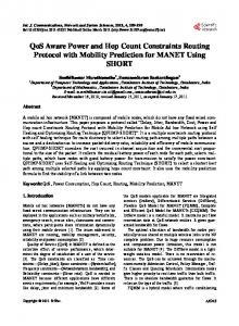
DARP Chapter 3 MO-DARP Chapter 4

HDARP Chapter 5 dHDARP Chapter 6

Figure 1.1: Outline

either be considered in terms of additional constraints or in terms of additional objectives. Both approaches are subject to investigation in this thesis. In a first step, a solution method based on Variable Neighborhood Search (VNS) (Mladenovic and Hansen, 1997) for a rather standard Dial-A-Ride Problem (DARP) version will be developed in Chapter 3. A vehicle fleet of fixed size, time windows, maximum user ride times, and a route duration limit are among the constraints considered. This “standard” DARP will be extended in two ways, as shown in Figure 1.1. In Chapter 4, besides routing costs, a user-oriented objective, minimizing user inconvenience, in terms of mean user ride time, will be introduced. This results in a problem version we will denote as Multi-Objective Dial-A-Ride-Problem (MO-DARP). An exact and a heuristic solution method will be devised. The heuristic solution method integrates VNS and Path Relinking (PR) (Glover and Laguna, 1997) in a two-phase scheme. The exact method iteratively solves single objective problems to optimality within a so-called ǫ-constraint framework (Laumanns et al., 2006). The developed procedures will provide the ambulance dispatcher with a number of transportation plans, which are incomparable across each other: neither will be better than any other transportation plan in both objectives. Information regarding their respective quality of service level as well as cost will be provided. In this case, the task of choosing a transportation plan out of the set of these efficient transportation plans is left with the person in charge. In Chapter 5, in order to decrease the gap between theory and practice, heterogeneous patient types and a heterogeneous vehicle fleet, as employed by the ARC, will be added to the standard dial-a-ride model, resulting in a Heterogeneous Dial-A-Ride Problem (HDARP). Two mathematical problem formulations will be presented. Each of these will serve as the basis for a branch and cut algorithm. The previously developed VNS will also be adapted to HDARP. In Chapter 6, the HDARP will be extended to the dHDARP, i.e. the heterogeneous dial-aride problem with driver related constraints, which corresponds to the real world ambulance routing problem faced by the ARC. Based on available information, staff related conditions will be introduced into the problem. These refer to the assignment of drivers and other

2

staff members to vehicles, and to the scheduling of lunch breaks and additional stops at the depot. An exact column generation procedure will be devised to compute lower bounds. These bounds will serve to assess the solution quality of the proposed VNS. In this case, further adaptations will be necessary in order to accommodate all real-world characteristics. This book is organized as follows. In Chapter 2, first, a classification scheme for vehicle routing problems with pickups and deliveries is proposed. Then, a short introduction to the different solution paradigms applied in this field is given. This is followed by a brief review of the different solution methods proposed for each problem class. Each of the four subsequent chapters is dedicated to one of the above described ambulance routing problems. Each chapter contains a formal definition of the problem, the description of the developed solution procedure(s), and computational results for up to three (adapted) data sets from the literature. In Chapter 6 also real world instances are considered. At the end of each chapter, a short summary of the respective findings is given. The book closes with a conclusion, summarizing the obtained results and indicating future research directions.

3

2 Summarizing the state-of-the-art 2.1 Introduction Over the past decades extensive research has been dedicated to modeling aspects as well as optimization methods in the field of vehicle routing. Especially transportation problems, involving both, pickups and deliveries, have received considerable attention. This is mainly due to the need for improved efficiency, as the traffic volume increases much faster than the street network grows (cf. Eurostat, 2004, 2006, for data on the European situation). Along with the increasing use of geographical information systems, companies seek to improve their transportation networks in order to tap the full potential of possible cost reduction. Ambulance routing problems, considering the transportation of people between pre-specified pickup and drop off locations, belong to the above mentioned problem class. The rapidly growing body of research in the field of vehicle routing involving pickups as well as deliveries has led to a somewhat confusing terminology. Indeed, the same problem types are denoted by various names and different problem classes are referred to by the same denotations. The problem we will denote traveling salesman problem with mixed backhauls, e.g., has been denoted as Traveling Salesman Problem (TSP) with pickup and delivery (Mosheiov, 1994), TSP with delivery and backhauls (Anily and Mosheiov, 1994), and as TSP with deliveries and collections (Baldacci et al., 2003). Its multi vehicle version has been referred to as mixed Vehicle Routing Problem (VRP) with backhauls (Ropke and Pisinger, 2006b; Salhi and Nagy, 1999), as VRP with backhauls with mixed load (e.g. Dethloff, 2002), and as pickup and delivery problem (Mosheiov, 1998). Despite the fact that the naming pickup and delivery problem has most often been used to refer to an entirely different problem class (see below). This situation calls for a clear classification scheme and naming. In this chapter we will introduce such a classification scheme. Thereafter, a short introduction to solution concepts (exact methods, heuristics, and metaheuristics) applied in the vehicle routing field will be given. This is followed by a condensed overview of solution methods developed in the pickup and delivery problem domain, following the developed classification scheme, while focusing on those works related to the static ambulance routing field. For further details on the different vehicle routing problem classes involving pickups as well as deliveries we refer to the two articles (Parragh et al., 2008a,b). They form the basis of this chapter. A recent work by Berbeglia et al. (2007) provides a different classification

5

2 Summarizing the state-of-the-art General Pickup and Delivery Problems (GPDP)

transportation from/to a depot (VRPB)

transportation between customers (VRPPD)

unpaired

TSPCB VRPCB

TSPMB VRPMB

TSPDDP VRPDDP

TSPSDP VRPSDP

PDTSP PDVRP

paired

SPDP PDP

SDARP DARP

Figure 2.1: A classification scheme

scheme and survey for static vehicle routing problems involving pickups as well as deliveries. This work has been compiled in parallel to our two-part article.

2.2 Classification We distinguish two problem classes. The first class refers to situations where all goods delivered have to be loaded at one or several depots and all goods picked up have to be transported to one or several depots. Problems of this class are usually referred to as VRP with Backhauls (VRPB), a term coined by Goetschalckx and Jacobs-Blecha (1989). The second class comprises all those problems where goods (passengers) are transported between pickup and delivery customers (points) and will be referred to as VRP with Pickups and Deliveries (VRPPD). The two pickup and delivery problem classes are depicted in Figure 2.1. Their subclasses are described in the following.

2.2.1 VRPB subclass definitions The VRPB can be further divided into four subclasses. In the first two subclasses, customers are either delivery or pickup customers but cannot be both. In the last two subclasses, each customer requires a delivery and a pickup. The first subclass is characterized by the requirement that the group or cluster of delivery customers has to be served before the first pickup customer can be visited. Delivery customers are also denoted as linehaul customers, pickup customers as backhaul customers. We will refer to this problem class as VRP with Clustered Backhauls (VRPCB). Its single vehicle case will be denoted as TSP with Clustered Backhauls (TSPCB). The second VRPB subclass does not consider a clustering restriction. Mixed visiting sequences are explicitly allowed. We will denote this problem class as VRP with Mixed

6

2.2 Classification linehauls and Backhauls (VRPMB) in the multi vehicle case, and TSP with Mixed linehauls and Backhauls (TSPMB) in the single vehicle case. The third VRPB subclass describes situations where customers can be associated with both a linehaul and a backhaul quantity but, in contrast to subclass four, it is not required that every customer is only visited once. Rather, two visits, one for delivery and one for pickup are possible. In this case, so called lasso solutions can occur, in which first a few customers are visited for delivery service only, in order to empty the vehicle partially. Then, in the “loop of the lasso”, customers are visited for both pickup and delivery service. In the end, the pickups are performed for the customers initially visited for delivery. We will refer to the single vehicle case as TSP with Divisible Delivery and Pickup (TSPDDP) and to the multi vehicle case as VRP with Divisible Delivery and Pickup (VRPDDP) in order to emphasize that a customer can either be visited once for both pickup and delivery or twice, first for delivery and then for pickup. The fourth VRPB subclass covers situations where every customer may be associated with a linehaul as well as a backhaul quantity. It is imposed that every customer can only be visited exactly once. We will denote this problem class as VRP with Simultaneous Delivery and Pickup (VRPSDP), its single vehicle version as TSP with Simultaneous Delivery and Pickup (TSPSDP).

2.2.2 VRPPD subclass definitions The class we denote VRPPD refers to problems where goods are transported from pickup to delivery points. It can be further divided into two subclasses (see Figure 2.1). The first subclass refers to situations where pickup and delivery locations are unpaired. A homogeneous good is considered. Each unit picked up can be used to fulfill the demand of any delivery customer. In the literature mostly the single vehicle case is tackled. Since also a multi vehicle application has been reported (see Dror et al., 1998) we will denote this problem class as Pickup and Delivery VRP (PDVRP) and Pickup and Delivery TSP (PDTSP), in the multi and in the single vehicle case, respectively. The second VRPPD subclass comprises the classical Pickup and Delivery Problem (PDP) and the Dial-A-Ride Problem (DARP). Both consider transportation requests, each associated with an origin and a destination, resulting in paired pickup and delivery points. The PDP deals with the transportation of goods while the DARP deals with passenger transportation. This difference is usually expressed in terms of additional constraints or objectives that take user (in)convenience into account. A majority of the work published denotes this problem class as Pickup and Delivery Problem (PDP) (see e.g. Dumas et al., 1991; van der Bruggen et al., 1993). We will follow this naming. Dial-a-ride problems are also mostly referred to as such. We denote the single vehicle case of the PDP as SPDP, the single vehicle case of the DARP as SDARP. All problems dealt with in the subsequent

7

2 Summarizing the state-of-the-art chapters of this book belong to the DARP class.

2.3 Solution methods In general, two different types of solution methods can be distinguished. These are exact algorithms yielding an optimal solution to the problem handled and heuristic algorithms, computing (hopefully) near optimal solutions within short or at least acceptable computation times.

2.3.1 Exact methods Exact solution methods applied to vehicle routing problems considering both pickups as well as deliveries involve well known solution paradigms in combinatorial optimization; such as, among others, branch and bound, branch and cut, and branch and price algorithms. In branch and bound algorithms, first the according Linear Programming (LP) relaxation to the respective problem formulated as a (mixed) Integer Program (IP) is solved. The solution of the LP relaxation will provide a lower bound for the solution of the original IP (in the context of minimization). In case the obtained solution is integer, the optimal solution to the original IP has been found. Otherwise, a branch and bound tree is built. From the root node two child nodes are generated by branching. At each child node, a new LP is solved with an additional constraint; either an upper or a lower bound on one of the variables which are supposed to be integer but are associated with a fractional value in the current solution is set. In the subsequent iterations each child node serves as the parent node for two new child nodes in the tree. The tree is explored in a branch and bound fashion; bounds are obtained by the optimal solution values to the LP at the nodes of the search tree. If the lower bound at some node of the search tree is greater than the upper bound obtained at another node, the former node can be excluded from the search. An alternative method to the branch and bound method is the so-called cutting plane algorithm. First, as in branch and bound, the LP relaxation of the original IP is solved. In case the obtained solution is not integer, a cut is generated that separates the optimal solution from the true feasible set. A valid cut has two properties. First, any feasible point of the IP satisfies the cut; and second, the current optimal solution to the LP will violate the cut (Winston, 1994). This is illustrated in Figure 2.2. The gray space corresponds to the feasible region of the LP relaxation; the black dots to the set of feasible solutions of the original IP. The dashed line represents the objective function. The optimal solution to the LP relaxation corresponds to the lower left corner of the feasible region and yields a lower bound. A cutting plane, as given by the dotted line, separates this solution but does not cut off any of the IP feasible points. Also the optimal solution of the original IP is shown (x1 = 1, x2 = 2). Cuts are thus iteratively added to the LP relaxation until an integer

8

2.3 Solution methods x2 6 b

5 b

b

b

b

4 b

b

b

b

3 b

b

b

b b

2 b

b

1

b

feasible LP space feasible IP point objective function cutting plane optimal solution

b

x1

0 0

1

2

3

4

5

6

Figure 2.2: A lower bound and a cutting plane

solution is obtained. Branch and cut methods combine the branch and bound and the cutting plane idea. In difference to branch and bound only a subset of the original constraints are considered in the LP relaxation. Typically, all constraint families of exponential size are not included. So-called separation algorithms will check the solution of the LP relaxation at the current node in the search tree for violations of the omitted constraints. In case none of the omitted constraints are violated, an optimal solution to the LP has been found. Otherwise, if at least one violated constraint has been detected by a separation procedure the violated constraint(s) is (are) added to the LP, and the updated LP is solved again. This is repeated until the separation procedures fail to detect additional violated constraints. A branch and cut algorithm will be employed to solve the heterogeneous dial-a-ride problem in Chapter 5. We refer to this chapter for further details. The column generation method has been introduced by Gilmore and Gomory (1961) to solve large scale LP. Its basic principle is that it is not necessary to consider all columns at once. The idea is to search in an efficient way for columns that will price out favorably by taking dual information into account. The Dantzig-Wolfe decomposition method uses this idea. It has been first introduced by Dantzig and Wolfe (1960) for LP. Many problems can be formulated in two ways: in terms of a so-called compact formulation (such as the 2-index and 3-index formulations of the DARP presented in the following chapters) and in terms of a so-called extensive formulation (such as, e.g, set partitioning type formulations). Compact formulations can be transformed into extensive formulations by means of decomposition. The extensive formulation usually contains less rows (constraints) but a lot more columns (variables) than the compact formulation. To solve the LP relaxation of the extensive formulation, column generation is used. In vehicle routing these columns usually refer to

9

2 Summarizing the state-of-the-art routes. Thus, the optimal combination out of the set of all feasible routes is searched. This set is usually too large to be considered at once. Therefore, so-called pricing procedures are used to identify favorable columns (pricing subproblem), by using dual information from the solution of the restricted master (i.e. the extensive formulation) considering the set of columns generated so far. The optimal solution to the original LP has been found if no additional favorable columns exist. For further information we refer to Desaulniers et al. (2005). This solution method is applied to the dial-a-ride problem variant considered in Chapter 6 of this book. Integrated into a branch and bound scheme, where each linear relaxation is solved by means of column generation, results in a so-called branch and price algorithm. In case also cuts are added (as in branch and cut) the resulting solution method is referred to as branch and cut and price. In case only a subset of the tree is considered or, e.g., in column generation only heuristic pricing procedures are applied, these exact methods are turned into heuristic procedures. Further information on exact solution algorithms can be found, e.g., in Barnhart et al. (1998); Fischetti and Toth (1989); Padberg and Rinaldi (1991).

2.3.2 Heuristics Following Semet and Laporte (2002), heuristic methods in the field of vehicle routing can be further divided into classical heuristics and metaheuristics. Classical heuristic methods comprise construction heuristics, two-phase heuristics, and improvement methods. Construction heuristics build a feasible solution, trying to keep the objective function value as low as possible (in the context of minimization). Once a (customer) location has been inserted, it is usually not removed again. Popular concepts belonging to this class are sequential and parallel insertion heuristics. Sequential heuristics only consider one route at a time, while parallel heuristics consider multiple routes at once. A popular insertion criterion is cheapest insertion; the (customer) location resulting in the least cost increase regarding the so far constructed partial solution is inserted next. Two-phase heuristics describe cluster-first-route-second and route-first-cluster-second implementations. In case of cluster-first-route-second, the (customer) locations are first assigned to routes, following some criterion and only then for each cluster (route) the order in which the (customer) locations are visited is determined. The reverse is done in case of route-first-cluster-second heuristics. Here, first a giant tour is constructed and only then this tour is segmented into as many clusters (routes) as necessary. Improvement heuristics either consider each vehicle route at a time (intra-tour) or several routes (inter-tour). Popular intra-tour improvement heuristics use the λ-opt mechanism of Lin (1965) (especially 2-opt and 3-opt). λ edges are removed from a route and the remaining route segments are reconnected in all possible ways. Every time an improved solution is encountered the according reconnection is kept. This is repeated until no further improve-

10

2.3 Solution methods ments are possible. The Or-opt (Or, 1976) method, e.g., relocates sequences consisting of 3, 2, and 1 vertices, resulting in a restricted form of 3-opt.

2.3.3 Metaheuristics The term metaheuristic has been used for the first time by Glover (1986) to refer to a tabu search heuristic. A metaheuristic distinguishes itself from a classical heuristic by some “meta” structure that allows the search to escape from local optima. Thus, intermediate infeasible or deteriorating solutions are allowed during the search. Metaheuristics in the field of vehicle routing often apply concepts of classical construction and improvement heuristics. Usually they find better local optima than classical heuristic methods but they also tend to need longer computation times (Gendreau et al., 2002). On the one hand, there are metaheuristic approaches that are population based or related to population based methods, such as genetic algorithms or ant colony optimization, and, on the other hand, there are methods that are based on different local search neighborhoods, such as tabu search, variable neighborhood search, or simulated annealing. The term neighborhood refers to all solutions that can be constructed by applying a certain local search operator (e.g. a simple vertex move) to a given solution. In genetic algorithms, in each iteration a population of solutions is considered. Every new population of solutions is obtained from the previous one by operators such as recombination and mutation, keeping the best (new) solutions and eliminating the worst. In ant colony optimization, in each iteration a construction heuristic is used to generate a number of new solutions based on information from previous iterations. One of the most popular metaheuristics is tabu search (Glover and Laguna, 1997). It works as follows. A simple neighborhood operator such as, e.g. an inter-tour vertex move is used to transform the current solution into a new solution. All possible moves are considered and the best non-tabu one is used to constitute a new solution. The reverse move of the one that was used to build the new solution is then set “tabu” for a certain number of iterations. The new solution may be worse than the previous solution. This concept allows the search to escape from local optima. In variable neighborhood search (Mladenovic and Hansen, 1997), several neighborhoods of different size are considered. Ideally, the smallest should be contained in the next larger one and so on. If the smallest neighborhood consists of all possible intertour moves of one vertex, the next larger neighborhood could consist of all possible moves of one and two vertices, and so on. In every iteration a new solution is constructed at random in the current neighborhood. Then some improvement heuristic is used to optimize this solution locally. In case it improves the current incumbent solution, it becomes the new incumbent and the search continues with the smallest neighborhood. Otherwise, the next larger neighborhood is considered and another random solution is constructed. Also ˘ in simulated annealing (Kirkpatrick et al., 1983; Cerny, 1985) in every iteration a random

11

2 Summarizing the state-of-the-art solution is constructed in a given neighborhood. In case this solution is better than the current incumbent, it becomes the new incumbent solution. Otherwise, it is accepted with a certain probability. This probability depends on the solution value of the new solution and a “temperature”. The “temperature” is decreased during the search according to a certain scheme. The “cooler” it gets the lower the probability that a deteriorating new solution is accepted as the new incumbent solution. The variable neighborhood search concept, integrating ideas from simulated annealing, will be used to solve the different ambulance routing problems considered in this book. For additional information we thus refer to the following chapters. Further information on local search methods can be found, e.g., in Aarts and Lenstra (1997), neighborhood based methods are discussed, e.g., in Br¨ aysy and Gendreau (2005); Funke et al. (2005) and metaheuristics in Hoos and St¨ utzle (2005).

2.4 Solution methods for VRPB The development of solution methods for VRPB is most probably motivated by the fact that combined linehaul and backhaul tours may result in less empty hauls and thus in possible cost reductions. Depending on the type of good transported, company policies, or customer preferences, backhauls may have to be done last, customers have to be visited only once, etc. In the following, first, research work dealing with the clustered version (all linehauls before backhauls) will be reviewed, this is followed, by the mixed case, the combined and divisible case (all customers may demand both services and can be visited twice), and the combined case with simultaneous service (all customers may demand both services but can only be visited once).

2.4.1 All linehauls before backhauls (TSPCB, VRPCB) The TSPCB can be viewed as a special case of the Clustered Traveling Salesman Problem (CTSP), where only two clusters are considered. The CTSP was first formulated in Chisman (1975). Already in Lokin (1978) an application of the CTSP to a backhaul problem is suggested. Thus, all solution algorithms for CTSP, e.g., those presented in Gendreau et al. (1996b); Jongens and Volgenant (1985); Laporte et al. (1996); Potvin and Guertin (1996), are also valid solution techniques for the TSPCB with the additional constraint that the set of linehaul customers is visited first. A survey covering the different VRPCB solution methods can be found in Toth and Vigo (2002). The first exact approach for the VRPCB is due to Yano et al. (1987). The proposed branch and bound method generates optimal routing plans with up to 4 linehaul and 4 backhaul customers per route. Further, more sophisticated branch and bound derived algorithms followed (G´elinas et al., 1995; Mingozzi et al., 1999; Toth and Vigo, 1997a). The latest are able to solve benchmark instances (Goetschalckx and Jacobs-Blecha, 1989; Toth and Vigo,

12

2.4 Solution methods for VRPB 1996b, 1999) with up to 100 customers to optimality . Quite a lot of research has been conducted in the field of heuristic methods for VRPCB. The solution paradigms applied range from simple as well as more sophisticated construction heuristics (Deif and Bodin, 1984; Derigs and Metz, 1992), to construction-improvement type implementations (Gendreau et al., 1996a; Goetschalckx and Jacobs-Blecha, 1989; Thangiah et al., 1996), and cluster-first-route-second methods (Anily, 1996; Min et al., 1992; Toth and Vigo, 1996b, 1999) applying well-known operators such as 2-exchange, 3-exchange (Lin, 1965), λ-interchange (Osman, 1993), 2-opt*-exchange (Potvin and Rousseau, 1995), or the GENI idea (Gendreau et al., 1992). Those research works that are among the most recent in the field of VRPCB, belong to the metaheuristic domain. The tabu search concept has been employed by Brand˜ ao (2006); Crispim and Brand˜ ao (2001); Duhamel et al. (1997); Osman and Wassan (2002). However, also neural networks (Ghaziri and Osman, 2003, 2006), genetic algorithms (Ganesh and Narendran, 2007; Potvin et al., 1996), an insertion based ant system (Reimann et al., 2002), guided local search (Zhong and Cole, 2005), simulated annealing (Hasama et al., 1998), variable neighborhood search (Crispim and Brand˜ ao, 2001; Mladenovic and Hansen, 1997), and adaptive large neighborhood search (Ropke and Pisinger, 2006b) have been used to solve different versions of VRPCB. Over the years with increasing computational power a shift from simple heuristic methods towards more sophisticated metaheuristic solution procedures can be observed. Thus, recent state-of-the-art methods in the field of VRPCB predominantly belong to the metaheuristic domain. Comparison can be done by looking at the different results achieved for the same set of benchmark instances. In case of the VRPCB without time windows, the benchmark instances most often used are the ones of Goetschalckx and Jacobs-Blecha (1989) (GJ89) and Toth and Vigo (1996b) (TV96). The largest instance solved to optimality of the GJ89 data set comprises 90 customers and in case of the TV96 data set 100 customers (see Mingozzi et al., 1999). The latest new best results for these data sets are reported in Ropke and Pisinger (2006b) and Brand˜ ao (2006). In case of the VRPCB with time windows the data set proposed in G´elinas et al. (1995) (GDDS95) is the prevalent one. The largest instance solved to optimality within this data set consists of 100 customers (cf. G´elinas et al., 1995). Most recent new best results have also been reported by Ropke and Pisinger (2006b).

2.4.2 Mixed linehauls and backhauls (TSPMB, VRPMB) We now turn to the VRPMB where linehaul and backhaul customers can occur in any order along the route. Exact solution methods for the VRPMB have only been developed for the single vehicle case. Tzoreff et al. (2002) present a linear time algorithm for tree graphs, and polynomial time algorithms for a cycle and a warehouse graph. S¨ ural and Bookbinder (2003) work on bounds of the linear relaxation and Baldacci et al. (2003) discuss valid inequalities

13

2 Summarizing the state-of-the-art and embed them into a branch and cut algorithm. The first solution methods proposed for the VRPMB belong to the field of heuristics. These are two heuristics using the Clarke-Wright algorithm (Clarke and Wright, 1964) to schedule the linehauls and different insertion procedures to insert the backhauls (Casco et al., 1988; Golden et al., 1985). A similar idea is also used by Wade and Salhi (2002). Salhi and Nagy (1999) extend the idea of Golden et al. (1985), introducing the notion of clusters and borderline customers in a multi-depot setting. Giant tour partitioning heuristics have been developed by Mosheiov (1998). Further solution methods involve a minimum spanning tree based procedure (Anily and Mosheiov, 1994), a TSP tour based algorithm, a cheapest feasible insertion algorithm (Mosheiov, 1994) for the single vehicle case, and an extension of the cheapest insertion heuristic (Dethloff, 2002) for the multi vehicle case. The constructionimprovement principle is applied by Nagy and Salhi (2005). Metaheuristics have not been applied as extensively to the VRPMB as to other problem types. The solution paradigms applied range from greedy randomized adaptive search (Kontoravdis and Bard, 1995), simulated annealing (Hasama et al., 1998), and ant systems (Reimann and Ulrich, 2006; Wade and Salhi, 2004) to a combination of tabu search and variable neighborhood descent (Crispim and Brand˜ ao, 2005) and adaptive large neighborhood search (Ropke and Pisinger, 2006b). The largest TSPMB instance solved to optimality is reported in Baldacci et al. (2003). It is a single vehicle instance of the data set provided by Gendreau et al. (1999), containing 200 customers. The VRPMB instances most widely used are those proposed by Salhi and Nagy (1999). Most recent improved results for these instances are given by Ropke and Pisinger (2006b), outperforming earlier results by Nagy and Salhi (2005).

2.4.3 Divisible delivery and pickup (TSPDDP, VRPDDP) This problem class is a mixture of the previously described VRPMB and the VRPSDP, subject to review in the next section. In contrast to the VRPMB, every customer can be associated with a pickup and a delivery quantity. However, these customers do not have to be visited exactly once. They can be visited twice, once for pickup and once for delivery service. Only little research has been explicitly dedicated to this problem class. However, all the solution methods designed for the VRPMB can be applied to VRPDDP instances if every customer demanding pickup and delivery service is modeled as two separate customers. Salhi and Nagy (1999) apply their cluster insertion algorithm to VRPSDP instances, resulting in solutions that may violate the one-single-visit-per-customer restriction. Thus, they actually solve a VRPDDP. Halskau et al. (2001), on the other hand, explicitly relax the VRPSDP to the VRPDDP. The aim is to create so-called lasso solutions, i.e. customers along the spoke are visited twice (first for delivery and second for pickup service). Customers along the loop are only visited once. Hoff and Løkketangen (2006) also study lasso solutions but restricted

14

2.4 Solution methods for VRPB to the single vehicle case. An in-depth study of different solution shapes for TSPDDP is conducted by Gribkovskaia et al. (2007); they consider lasso, Hamiltonian, and double-path solutions. The concept of “general solutions” is introduced. Their work is motivated by the fact that additional cost reductions can be realized when relaxing the VRPSDP to the VRPDDP. The proposed methods are classical construction and improvement heuristics and a tabu search algorithm. They are tested on instances containing up to 100 customers. The results show that the best solutions obtained are often non-Hamiltonian and may contain up to two customers that are visited twice.

2.4.4 Simultaneous delivery and pickup (TSPSDP, VRPSDP) The difference between VRPDDP and VRPSDP refers to customers demanding pickup and delivery service. In case of the VRPSDP these customers have to be visited exactly once for both services. The VRPMB is a special case of the VRPSDP where every customer only demands a pickup or a delivery but not both. This problem class was first defined by Min (1989). The only exact algorithm for the VRPSDP with time windows is presented in Angelelli and Mansini (2002). Based on a set covering formulation of the master problem a branch and price approach is designed. Dell’Amico et al. (2006) also propose a branch and price algorithm to solve the VRPSDP but without time windows. They use a hierarchy based on five pricing procedures: four heuristics and one exact method. Several heuristic methods for different versions of the VRPSDP can be found in the literature. Construction-improvement algorithms for the single vehicle case have been developed by Gendreau et al. (1999) and Alshamrani et al. (2007). Both are based on TSP cycles, improved using arc-exchanges, or the Or-opt operator. The latter considers a periodic version and stochastic demand figures. Gendreau et al. (1999) compare the construction algorithms of Mosheiov (1994) and Anily and Mosheiov (1994) to a cheapest feasible insertion heuristic. A cheapest insertion based algorithm for the multi vehicle case is also used by Dethloff (2001). The cluster-first-route-second idea is applied by Halse (1992) and Min (1989). Also metaheuristic solution methods have been applied to the VRPSDP. The first metaheuristic for the TSPSDP is a tabu search algorithm using a 2-exchange neighborhood (Gendreau et al., 1999). Tabu search has also been applied to the multi vehicle version (see Bianchessi and Righini, 2007; Tang Montan´e and Galv˜ao, 2006). Chen and Wu (2006) integrate a tabu list into a record to record algorithm, a hybrid between a tabu search and a variable neighborhood descent algorithm is described in Crispim and Brand˜ ao (2005) Again the same trend as for VRPMB can be observed. Early research favored simple heuristic algorithms whereas recent algorithms mostly belong to the field of metaheuristic solution procedures. The largest VRPSDP instance solved to optimality comprises 40 requests (Dell’Amico et al., 2006); however, no standard benchmark instance is considered.

15

2 Summarizing the state-of-the-art Two data sets have been most often referred to. These are those of Salhi and Nagy (1999) (SN99b) and Dethloff (2001) (Det01). The best pooled results for the SN99b instances hold Ropke and Pisinger (2006b) and Nagy and Salhi (2005). Tang Montan´e and Galv˜ao (2006) also report improved solutions, however, not the whole set is considered. Consequently, a direct comparison to the other two is impossible. For the Det01 data set Ropke and Pisinger (2006b), Tang Montan´e and Galv˜ao (2006), and Bianchessi and Righini (2007) obtain new best results of similar quality, but present them in different pooled form, only comparing themselves to the results of Dethloff (2001). Whatever method produces the best results, all of them are metaheuristics, clearly indicating that these more sophisticated methods outperform straightforward heuristic procedures.

2.5 Solution methods for VRPPD In the following section an overview of the different solution methods for the PDVRP, the PDP, and the DARP, forming the second class of vehicle routing problems involving pickups and deliveries, are presented. Solution methods again classify into exact, heuristic, and metaheuristic approaches. In all previously described problem classes, goods were loaded at the depot and delivered to different locations, and picked up at different locations and returned to the depot. All problem classes described in the following deal with situations where goods are transported between pickup and delivery customers. In the first problem class, an identical good is considered. Thus, every customer’s demand may be fulfilled by every other customer’s supply. In the last two problem classes pickup and delivery points are paired and the goods transported may or may not be identical. In the last class instead of goods, people are subject to transportation. The focus will lie on the last class (DARP). All ambulance routing problems discusses in the following chapters belong to this problem class.

2.5.1 Unpaired pickups and deliveries (PDVRP, PDTSP) The PDVRP, i.e. the problem class where every good can be picked up and transported anywhere, did not receive as much attention in the literature as the other problem classes. Moreover, most of the literature is restricted to the PDTSP. Therefore, with the exception of Dror et al. (1998), all solution methods presented are only applicable to the one vehicle case. To the authors’ knowledge no metaheuristic approach for the PDTSP has been proposed until today. The only exact method proposed for the problem at hand has been introduced by Hern´andezP´erez and Salazar-Gonz´alez (2003, 2004a), using a branch and cut framework. The test instances solved are adaptations of the ones used in Mosheiov (1994) and Gendreau et al. (1999), containing up to 75 customers. This branch and cut algorithm is also used as a

16

2.5 Solution methods for VRPPD heuristic in an incomplete optimization scheme (Hern´andez-P´erez and Salazar-Gonz´alez, 2004b). A construction-improvement type algorithm, applying a greedy construction procedure, improved by 2-opt and 3-opt exchanges is proposed in the same paper. A special case of the PDTSP is considered in Chalasani and Motwani (1999); the number of goods to be picked up is equal to the number of goods to be delivered; the demand (supply) at every delivery (pickup) location is equal to one. This problem is an extension of the swapping problem where the vehicle’s capacity is also set to one. Chalasani and Motwani propose an approximation algorithm with a worst case bound of 9.5. Anily and Bramel (1999) devise a polynomial time iterated tour matching algorithm for the same problem. An approximation algorithm on a tree graph with a worst case bound of 2 is developed in Lim et al. (2005). The PDTSP on a tree and on a line is also subject to investigation in Wang et al. (2006). They propose an O(|V |2 / min {C, |V |}) algorithm for the line case. The unit capacity as well as the uncapacitated version can be solved in linear time. On a tree an O(|V |) algorithm is devised for the case of unit capacity and an O(|V |2 ) algorithm for the uncapacitated case. |V | gives the number of vertices and C the vehicle capacity. Finally, Dror et al. (1998) propose a heuristic algorithm for the application of the PDVRP to the redistribution of self-service cars. It is related to Dijkstra’s algorithm (Dijkstra, 1959). Also other solution approaches are briefly discussed.

2.5.2 Pickup and delivery problems (SPDP, PDP) Solution methods for the classical PDP, where every transportation request is associated with a pickup and a delivery point, are presented in this section. Lokin (1978) was the first to discuss the incorporation of precedence constraints into the traditional TSP, needed to formulate the PDP. The first attempt to generalize the PDP in unified notation was proposed by Savelsbergh and Sol (1995), covering all possible versions of the PDP, including the DARP. They also provide a brief overview of existing solution methods until 1995. Mitrovi´c-Mini´c (1998) present a survey on the PDP with Time Windows (PDPTW). An early survey on vehicle routing problems, already including the PDP is given in Desrochers et al. (1988). Cordeau et al. (2004) review demand responsive transport, covering PDP and DARP. Further surveys on solution methods can be found in Assad (1988); Desaulniers et al. (2002); Desrochers et al. (1988). In contrast to all problem classes discussed so far, in case of PDP and also DARP, in addition to the various static problem versions, also dynamic variants exist. The term “dynamic” refers to situations were only some requests are known ahead of the planning period. A major part, however, comes in during the planning period and has to be scheduled “on-line”. In the following paragraphs the various solution techniques for the static PDP are summarized according to exact, heuristic, and metaheuristic approaches. Thereafter, the different dynamic approaches are briefly discussed.

17

2 Summarizing the state-of-the-art 2.5.2.1 Static variants A number of exact solution procedures have been presented for the static PDP. Ruland and Rodin (1997) present a branch and cut algorithm to solve the SPDP. A branch and bound algorithm and various valid inequalities for the single vehicle PDPTW with Last-InFirst-Out (LIFO) loading, i.e. goods have to be delivered in the reverse order they were picked up, is reported in Cordeau et al. (2006). The first exact solution method applicable to both the single as well as the multi vehicle case dates back to Kalantari et al. (1985). The branch and bound algorithm described is an extension of the one developed by Little et al. (1963). Another branch and bound algorithm and valid inequalities are discussed in Lu and Dessouky (2004). Column generation approaches have also been applied to the PDPTW (Desrosiers and Dumas, 1988; Dumas et al., 1991; Sigurd et al., 2004). A branch and cut algorithm departing from two different 2-index PDPTW formulations is studied in Ropke et al. (2007). A branch and cut and price approach, i.e. valid inequalities are added in a branch and cut fashion, and their impact on the structure of the pricing problem is discussed in Ropke and Cordeau (2008). For further details we refer to a survey by Cordeau et al. (2007), covering recent work on PDP while focusing on exact approaches. Heuristics for the static PDP have first been proposed in the 1980s. Sexton and Choi (1986) use Bender’s decomposition procedure to solve the static SPDP approximately. Construction-improvement heuristics for the SPDP are discussed in Renaud et al. (2000); van der Bruggen et al. (1993), using exchange, deletion, and re-insertion operators (e.g. 4-opt* (Renaud et al., 1996)) in the improvement phase. Perturbation heuristics have been employed by Renaud et al. (2002); a sophisticated construction procedure for the multi vehicle case by Lu and Dessouky (2006). The idea of mini-clusters has also been used (Shang and Cuff, 1996; Thangiah and Awan, 2006). A so-called “squeaky wheel” iterative insertion procedure has been developed by Lim et al. (2002); Xu et al. (2003) propose a column generation based heuristic algorithm, considering several real world motivated constraints. A construction-improvement heuristic for the multi vehicle case with transshipment is presented in Mitrovi´c-Mini´c and Laporte (2006). In the metaheuristic domain mostly the PDP with time windows is considered. In the single vehicle case, a (probabilistic) tabu search (Landrieu et al., 2001) and a variable neighborhood search heuristic (Carrabs et al., 2007) have been used. The latter considers an additional constraint regarding rear loading (items can only be delivered in the reverse order they were picked up). A multi vehicle version including this constraint is solved by means of a greedy randomized adaptive search procedure (Ambrosini et al., 2004). Otherwise, mostly heuristics using the tabu search paradigm (Caricato et al., 2003; Lau and Liang, 2001, 2002; Nanry and Barnes, 2000) and evolutionary techniques, such as genetic algorithms or indirect search, (Creput et al., 2004; Derigs and D¨ohmer, 2008; Jung and Haghani, 2000; Pankratz, 2005; Sch¨ onberger et al., 2003) have been used to solve different versions of the PDP. Most

18

2.5 Solution methods for VRPPD of them consider time windows. Also two hybrid algorithms have been reported in the literature, combining simulated annealing with tabu search (Li and Lim, 2001), and with large neighborhood search (Bent and van Hentenryck, 2006). Large neighborhood search has also been successfully applied in combination with an adaptive removal and insertion procedure selection scheme (Ropke and Pisinger, 2006a). Summarizing, the largest static PDP problem instance solved to optimality with a state-ofthe-art method comprises 205 requests (Sigurd et al., 2004). However, the size of the largest instance solved is not always a good indicator; tightly constrained problems are easier to solve than less tightly constrained ones. The benchmark data set most often used to assess the performance of (meta)heuristic methods for the static PDPTW is the one described in Li and Lim (2001) (LL01, LL01+). Recent new best results have been presented in Ropke and Pisinger (2006a) and Bent and van Hentenryck (2006), two metaheuristic solution procedures. The metaheuristic of Li and Lim (2001) still holds the best results for a part of the smaller instances. However, also exact methods advanced; the more tightly constrained part of the LL01 data set has recently been solved by a state-of-the-art branch and cut and price algorithm (Ropke and Cordeau, 2008). 2.5.2.2 Dynamic and stochastic variants Although many real world PDP are inherently dynamic, the dynamic version of the PDP has not received as much attention as its static counterpart. The term dynamic usually indicates that the routing and scheduling of requests has to be done in real time; new requests come in dynamically during the planning horizon and have to be inserted into existing partial routes. In general, the same objectives as for the static PDP are applied, e.g. the minimization of total operating costs. Surveys on dynamic routing can be found in Ghiani et al. (2003); Psaraftis (1988). In stochastic variants of the PDP, information regarding a certain part of the data (e.g. vehicle travel times) are only available in terms of probability distributions. So far, exact procedures have not been used to solve dynamic or stochastic PDP. Swihart and Papstavrou (1999) solve a stochastic SPDP. They test three routing policies, a sectoring, a nearest neighbor and a stacker crane policy. Lower bounds on the expected time a request remains in the system under light and heavy traffic conditions are computed. Three online algorithms (REPLAN, IGNORE, and SMARTSTART) for a single server PDP are investigated in Ascheuer et al. (2000b). The objective considered is the completion time. In the literature the problem at hand is called online dial-a-ride problem. However, the denotation dial-a-ride problem is not used in the same way as defined in this book. The term online is used whenever no request is known in advance. By means of competitive analysis, i.e. the online (no knowledge about the future) algorithm is compared to its offline (complete knowledge about the future) counterpart (Jaillet and Stafford, 2001; Van Hentenryck and Bent, 2006), it can be shown that REPLAN and IGNORE are 5/2 competitive, while SMARTSTART has a competitive ratio of 2. Hauptmeier et al. (2000) discuss the

19

2 Summarizing the state-of-the-art performance of REPLAN and IGNORE under reasonable load. Feuerstein and Stougie (2001) devise another 2-competitive algorithm. A probabilistic version (Coja-Oghlan et al., 2005) and the online problem minimizing maximum flow time (Krumke et al., 2005) are also investigated. Lipmann et al. (2004) study the influence of restricted information on the multi server online PDP, i.e. the destination of a request is only revealed after the object has been picked up. Competitive ratios of two deterministic strategies (REPLAN and SMARTCHOICE) for the time window case are computed in Yi and Tian (2005).

A heuristic using incomplete optimization for the dynamic multi vehicle PDP is proposed in Savelsbergh and Sol (1998). The solution methodology called DRIVE (Dynamic Routing of Independent VEhicles) incorporates a branch and price algorithm based on a set partitioning problem formulation. An insertion based heuristic using different types of order circuity control is discussed in Popken (2006). Fabri and Recht (2006) present an adaptation of a heuristic, initially designed for the dynamic DARP by Caramia et al. (2002).

Early research on dynamic multi vehicle PDP is conducted in Shen et al. (1995) and Potvin et al. (1995). Both articles focus on neural networks with learning capabilities to support vehicle dispatchers in real-time. A hybrid population based method, combining a genetic with a dynamic programming algorithm, for the dynamic SPDP with time windows is proposed in Jih and Hsu (1999). The first neighborhood based metaheuristic solution method for the dynamic multi vehicle PDPTW is presented in Malca and Semet (2004). A two-phase solution procedure is described in Mitrovi´c-Mini´c and Laporte (2004). In the first phase an initial solution is constructed via cheapest insertion and improved by means of a tabu search algorithm. In the second phase different waiting strategies are used to schedule the requests. The tested waiting strategies (drive first, wait first, dynamic waiting, advanced dynamic waiting) differ regarding the vehicle’s location when waiting occurs. Advanced dynamic waiting is also used by Mitrovi´c-Mini´c et al. (2004) in a double horizon based heuristic. The routing part is again solved by means of a construction heuristic improved by tabu search. Another tabu search algorithm for the dynamic multi vehicle PDPTW has been proposed by Gendreau et al. (2006), using an ejection chain neighborhood (Glover, 1996). Gutenschwager et al. (2004) compare a steepest descent, a reactive tabu search, and a simulated annealing algorithm.

To summarize, over the past decades, in the field of dynamic PDP, a number of solution procedures have been developed. However, the proposed algorithms cannot be directly compared since, so far, no standardized simulation environment has been used by more than one group of authors. Benchmark instances are available; e.g. those used by Mitrovi´cMini´c et al. (2004); Mitrovi´c-Mini´c and Laporte (2004).

20

2.5 Solution methods for VRPPD

2.5.3 Dial-a-ride problems (SDARP, DARP) The last problem class dealt with in this chapter is the dial-a-ride problem class. It has received considerable attention in the literature. The first publications in the field of passenger transportation date back to the late 1960s and early 1970s (cf. Rebibo, 1974; Wilson and Colvin, 1977; Wilson et al., 1971; Wilson and Weissberg, 1967). Additional information in the form of literature surveys on the different solution methods can be found in Cordeau and Laporte (2003a, 2007); Cordeau et al. (2004); Gendreau and Potvin (1998). As in the PDP class we distinguish between static and dynamic variants. The focus is put on the static part. All subsequent chapters deal with different problem variants belonging to the field of static DARP. 2.5.3.1 Static variants As in the previous sections we distinguish between exact, heuristic, and metaheuristic approaches. Given the vast amount of research published in the field of DARP, an overview of the different heuristic and metaheuristic approaches is given in tabular form. Exact methods Early research in the field of exact methods for the static SDARP predominantly belongs to the dynamic programming domain. An early exact dynamic programming algorithm for the SDARP is introduced in Psaraftis (1980). Service quality is taken care of by means of maximal position shift constraints compared to a first-come-first-serve visiting policy. A modified version of the above algorithm, considering time windows, is discussed in Psaraftis (1983b). Instead of backward recursion forward recursion is applied. A forward dynamic programming algorithm for SDARP is also discussed in Desrosiers et al. (1986). Possible states are reduced by eliminating those that are incompatible with respect to vehicle capacity, precedence, and time window restrictions. User inconvenience in terms of ride times is incorporated into time window construction, resulting in tight time windows at both, origin and destination of the transportation request. Kikuchi (1984) develop a balanced linear programming transportation problem for the multi vehicle DARP, minimizing empty vehicle travel as well as idle times and thus fleet size. In a pre-processing step the service area is divided into zones, the time horizon into time periods. Every request is classified according to an origin and a destination zone as well as a departure and an arrival time period. A branch and cut algorithm based on a 3-index formulation has been proposed by Cordeau (2006). New valid inequalities as well as previously developed ones for the PDP and the VRP are employed. The largest instance solved to optimality comprises 36 requests. Two branch and cut algorithms are described in Ropke et al. (2007). Instead of a 3-index formulation, two more efficient 2-index problem formulations and additional valid inequalities are employed. These two articles, presenting the most recent exact algorithms in the static DARP field,

21

2 Summarizing the state-of-the-art form the basis of the branch and cut algorithm for the DARP with heterogeneous fleet and passengers discussed in Chapter 5 of this book. Further details regarding the different families of valid inequalities employed can be found in the same chapter. Heuristics Over the past decades, a large number of heuristic algorithms have been proposed for the static DARP. Table 2.1 gives an overview of the various solution methods reported in chronological order, divided into single and multi vehicle approaches. For each entry the according literature reference, objective(s), and additional constraints considered are provided. Furthermore, either the benchmark instances used, or the size of the largest instance solved to optimality, in terms of number of requests, are given. A heuristic routing and scheduling algorithm for the SDARP using Bender’s decomposition is described in Sexton and Bodin (1985a,b). The scheduling problem can be solved optimally; the routing problem is solved with a heuristic algorithm. Other heuristic methods dealing with the single vehicle case involve a minimum spanning tree heuristic (Psaraftis, 1983a), adaptations of 2-opt and 3-opt heuristics (Psaraftis, 1983c), and a 2-opt improvement scheme switching between optimizing and sacrificing phases (Healy and Moll, 1995). One of the first heuristic solution procedures for a static multi vehicle DARP is discussed in Cullen et al. (1981). They develop an interactive algorithm that follows the clusterfirst-route-second approach. It is based on a set partitioning formulation solved by means of column generation. The location-allocation subproblem is only solved approximately. Other cluster-first-route-second approaches for different versions of the DARP are due to Bodin and Sexton (1986); Psaraftis (1986); Stein (1978a,b); Wolfler Calvo and Colorni (2007). A classical cluster-first-route-second algorithm has also been proposed by Bornd¨ orfer et al. (1997). Here, the clustering as well as the routing problem are modeled as set partitioning problems. The clustering problem can be solved optimally while the routing subproblems are solved approximately by a branch and bound algorithm (only a subset of all possible tours is used). Customer satisfaction is taken into account in terms of punctual service; customer ride times are implicitly considered by means of time windows. An optimization based mini-clustering algorithm is presented in Ioachim et al. (1995). It uses column generation to obtain mini-clusters and an enhanced initialization procedure to decrease processing times. As in Desrosiers et al. (1988) also the case of multiple depots is considered. The idea of mini-clusters has also been employed by Desrosiers et al. (1988, 1991); Dumas et al. (1989). Jaw et al. (1986) propose a sequential insertion procedure. First, customers are ordered by increasing earliest time for pickup. Then, they are inserted according to the cheapest feasible insertion criterion. The notion of active vehicle periods is used. Other construction heuristics have been proposed by Alfa (1986); Kikuchi and Rhee (1989); Roy et al. (1985a,b). A multi-objective approach is followed in Madsen et al. (1995). They discuss an insertion based algorithm called REBUS. The objectives considered are the total driving time, the

22

2.5 Solution methods for VRPPD

Table 2.1: Heuristics for the static DARP Reference

Type

Obj.

Constr.

Algorithm

Bench./ Size

The single vehicle case Psaraftis (1983a)

-

min. RC

-

MST heur., local interchanges

up to 50 req.

Psaraftis (1983c)

-

min. RC

-

adapted 2-opt and 3-opt

up to 30 req.

Sexton and Bodin (1985a,b)

-

min. CI

DDT

routing and scheduling algorithm based on Bender’s decomposition

up to 20 req.

Healy and Moll (1995)

-

min. RC

-

2-opt improvement, optimizing/sacrificing phases

up to 100 req.

The multi vehicle case Stein (1978a,b)

transfers

min. RC

TW

cluster first route second

-

Cullen et al. (1981)

-

min. RC

-

cluster first route second, column generation

up to 50 req.

Roy et al. (1985a,b)

HF

min. RC, min. CI

TW

parallel insertion

up to 578 req.

Bodin and Sexton (1986)

-

min. CI

DDT

cluster first route second

up to 85 req.

Jaw et al. (1986)

-

min. RC, min. CI

TW, RT

sequential feasible insertion algorithm

up to 2617 req.

Alfa (1986)

HF

min. RC

TW, RT

adapted heur. of (Jaw et al., 1986)

up to 49 req.

Psaraftis (1986)

-

min. RC, min. CI

TW, RT

comparison of Jaw’s heur. and grouping-clustering- routing heur.

-

Desrosiers et al. (1988); Dumas et al. (1989)

MD

min. RC

TW

mini-clustering algorithm, column generation

up to 200 req.

Kikuchi and Rhee (1989)

-

max. NCS

TW

sequential insertion

up to 200 req.

Desrosiers et al. (1991)

HF

min. RC

TW, RD

improved mini- clustering algorithm of (Desrosiers et al., 1988)

up to 2411 req.

Potvin and Rousseau (1992)

-

min. RC

TW, RT

constraint directed search (beam search)

up to 90 req.

Ioachim et al. (1995)

HF, MD, S

min. NV, min. RC

TW

mini-clustering, column generation

up to 2545 req.

Madsen et al. (1995)

HF, S

TW, RD, min. RC, NV, RT TWT, DPS

REBUS. insertion based algorithm up to 300 req.

Toth and Vigo (1996a)

HF

min. RC

TW, RT

parallel insertion, improved by trip insertion, exchange, double insertion, moves

TV96a

min. RC

TW, RD, (RT)

cluster first route second, set partitioning, branch and bound

up to 1771 req.

Bornd¨ orfer et al. HF, MD, (1997) S continued on next page

23

2 Summarizing the state-of-the-art Bench./ Size

Reference

Type

Obj.

Constr.

Algorithm

Diana and Dessouky (2004)

-

min. RC, min CI, idle times

TW, RT

parallel regret insertion heur.

up to 1000 req.

Xiang et al. (2006)

HF, S

min. RC

TW, RT, RD, BR

construction-improvement; clustering by TW, ideas of sweep heur.; local search improvement

up to 2000 req.

Wong and Bell (2006)

HF, S

min. RC, min. CI

TW, RT, RD

parallel insertion, improved by trip insertion

up to 150 req.

up to 180 TW cluster first route second, max. req. assignment heur., vertex NCS, reinsertions max. SL Bench. = Benchmark, BR = BReak time between two trips, CI = Customer Inconvenience, Constr. = Constraints, DDT = Desired Delivery Time, DPS = Deviation from Promised Service, HF = Heterogeneous Fleet, heur. = heuristic(s), MD = Multi Depot, NCS = Number of Customers Served, NV = Number of Vehicles, Obj. = Objective(s), RC = Routing Cost, RD = Route Duration, req. = requests, TW = Time Windows, TWT = Total Waiting Time, RT = Ride Time, S = Service time, SL = Service Level; The respective benchmark instances are described in Section 2.6. Wolfler Calvo and Colorni (2007)

-

number of vehicles, the total waiting time, the deviation from promised service times as well as cost. The regret insertion based process is also subject to analysis in a study by Diana (2004); in order to determine why the performance of this heuristic is superior to that of other insertion rules. The construction-improvement concept has also been used to solve the DARP (see Toth and Vigo, 1996a; Wong and Bell, 2006; Xiang et al., 2006). In the improvement phase operators such as trip insertion, exchange, and move are employed. Also beam search has been used to solve the multi-vehicle DARP (Potvin and Rousseau, 1992). Metaheuristics A much smaller number of metaheuristic solution methods have been developed for the static DARP. Table 2.2 provides an overview of the different algorithms proposed. For each reference the same information as in the previous table is given. Among the most popular metaheuristic concepts applied to the DARP are simulated annealing (Baugh et al., 1998; Colorni et al., 1996), tabu search (Aldaihani and Dessouky, 2003; Cordeau and Laporte, 2003a; Melachrinoudis et al., 2007), and genetic algorithms (Jørgensen et al., 2007; Rekiek et al., 2006; Uchimura et al., 1999). Toth and Vigo (1997b) describe a further local search based metaheuristic, a tabu thresholding algorithm, employing the neighborhoods defined in Toth and Vigo (1996a). In this book a variable neighborhood search algorithm will be developed and applied to different versions of the DARP. In Chapter 3 it is compared to the tabu search algorithm proposed by Cordeau and Laporte (2003b). They consider time windows at either origin or destination depending on the type of request (inbound or outbound). The neighborhood used is defined by moving one request to another route. The best possible move serves to generate a new incumbent solution. Reverse moves are declared tabu. However, an aspiration criterion is defined, such that tabu moves that provide a better solution, with respect to all other solutions already constructed

24

2.5 Solution methods for VRPPD

Table 2.2: Metaheuristics for the static DARP Reference

Type

Obj.

Constr.

Algorithm

Bench./ Size

The multi vehicle case Colorni et al. (1996)

-

max. NCS, min CI

RD

simulated annealing

up to 100 req.

Toth and Vigo (1997b)

HF, MD

min. RC

TW, RT

parallel insertion algorithm, tabu thresholding

TV96a

Baugh et al. (1998)

-

min. NV, min. RC, min. CI

TW

simulated annealing

up to 300 req.

Uchimura et al. (1999)

-

min. RC

RT, RD

genetic algorithm

10 req.

Cordeau and Laporte (2003b)

S

min. RC

TW, RT, RD

tabu search

CL03, up to 295 req.

Aldaihani and Dessouky (2003)

mix with FRT

min. RC, min. CI

TW

tabu search

up to 155 req.

Melachrinoudis et al. (2007)

HF, MD

min. RC, min CI

TW

tabu search

up to 8 req.

Rekiek et al. (2006)

S, MD, HF

min. NV, min. CI

TW, RT, VA

grouping genetic algorithm

up to 164 req.

Jørgensen et al. (2007)

S

min. RC, min. RT, min. TWV, ...

TW, RT, RD

genetic algorithm, space-time nearest neighbor heur.

CL03

Bench. = Benchmark, CI = Customer Inconvenience, Con. = Constraints, FRT = Fixed Route Transit, HF = Heterogeneous Fleet, MD = Multi Depot, mRT = mean RT, NV = Number of Vehicles, Obj. = Objective(s), RD = Route Duration, RT = Ride Time, RC = Routing Cost, S = Service time, TW = Time Windows, TWV = TW Violation, VA = Vehicle Availability; The respective benchmark instances are described in Section 2.6.

by the same move, can constitute a new incumbent solution. Summary State-of-the-art exact methods for the static DARP solve some instances with up to 96 requests to optimality (Ropke et al., 2007). However, the same limitation applies as mentioned above. The size of the test instance is not a very meaningful indicator; tightly constrained instances are easier to solve than those with less tight constraints and no standardized data set has been solved by the proposed approaches. In case of heuristic and metaheuristic methods, comparison becomes even harder since a large part of the solution procedures developed are motivated by real world problem situations. They differ regarding problem type (single and multi depot, homogeneous and heterogeneous fleet), constraints, and objective(s). Moreover, even when the same data sets are used different objectives are considered (see e.g. Cordeau and Laporte, 2003a; Jørgensen et al., 2007). Consequently, we can only state that in general heuristic methods run faster whereas metaheuristics usually outperform basic heuristic procedures with respect to solution quality. Related work Dealing with the transportation of people, especially handicapped or elderly, research has also been dedicated to the comparison of dial-a-ride systems with other modes of

25

2 Summarizing the state-of-the-art transportation. Early studies of dial-a-ride transportation systems are reported in Carlson (1976); Teixeira and Karash (1975). Elmberg (1978) test a robot dispatcher dial-a-ride system in Sweden. Daganzo (1984) compare fixed route transit systems with checkpoint dial-a-ride and door-to-door dial-a-ride systems. He concludes that most of the time either a fixed route system or door-to-door transportation is the appropriate choice. Belisle et al. (1986) investigate the impact of different operating scenarios on the quality of transportation systems for the handicapped. More recent studies comparing dial-a-ride and traditional bus systems by means of simulation are reported in Noda (2005); Noda et al. (2003). Shinoda et al. (2003) study the usability of dial-a-ride systems in urban areas. Mageean and Nelson (2003) evaluate telematics based demand responsive transport services in Europe. Palmer et al. (2004) analyze the impact of management practices and advanced technologies in the context of demand responsive transport systems. The impact of information flows, e.g. the percentage of real time requests or the length of the interval between the arrival of a new request and its requested pickup time window, is investigated in Diana (2006). Diana et al. (2006) study optimal fleet sizes with respect to predetermined service quality. Research has also been dedicated to possible ways of computation time reduction. Hunsaker and Savelsbergh (2002), e.g., propose a fast feasibility check for the DARP. The proposed procedure can deal with time window, waiting time as well as ride time restrictions. Castelli et al. (2002) discuss three algorithms granting 2-opt-improvement feasibility. 2.5.3.2 Dynamic and stochastic variants Less research has been dedicated to the domain of dynamic and/or stochastic DARP. Again, the term dynamic indicates that routing is done in real time; new requests pop up dynamically during the day and have to be scheduled into existing routes. Predominantly heuristic methods have been used to solve dynamic versions of the DARP. Exact methods have not been explicitly developed for the dynamic DARP. A possible reason is that, in the context of dynamic routing, the concept of “optimal solutions” becomes debatable. However, in Psaraftis (1980) the static version of their algorithm is adapted to the dynamic case. In a cluster-first-route-second framework Colorni and Righini (2001), considering only the most urgent requests, solve the routing subproblems to optimality with a branch and bound algorithm. Also Caramia et al. (2002) iteratively solve the single vehicle subproblems to optimality, using a dynamic programming algorithm. Another cluster-firstroute-second approach, applying dynamic programming in the routing phase, is reported in Dial (1995). New transportation requests are assigned to clusters according to least cost insertion. Teodorovic and Radivojevic (2000) propose a two-stage fuzzy logic based heuristic algorithm also following the cluster-first-route-second idea. The first approximate reasoning heuristic decides which vehicle a new request is assigned to. The second heuristic handles the adjustment of the vehicle’s route. Daganzo (1978) analyze three different insertion heuristics. In the first the closest stop

26

2.6 Benchmark instances is visited next. The second consists in visiting the closest origin or the closest destination in alternating order. The third only allows the insertion of delivery locations after a fixed number of passengers have been picked up. Horn (2002a) provide a software environment for fleet scheduling and dispatching of demand responsive services. The system can handle advance as well as immediate requests. New incoming requests are inserted into existing routes according to least cost insertion. A steepest descent improvement phase is run periodically. Also automated vehicle dispatching procedures, to achieve a good combination of efficient vehicle deployment and customer service, are included. The system was tested in the modeling framework LITRES-2 (Horn, 2002b). Another simulation environment to test solution methods for the dynamic DARP can be found in Fu (2002b). Coslovich et al. (2005) propose a two-phase insertion heuristic. A simple insertion procedure allows for quick answers with respect to inclusion or rejection of a new customer. The initial solution is improved by means of local search using 2-opt arc swaps. A dynamic DARP in a stochastic environment is considered in Xiang et al. (2007), taking into account travel time fluctuations, absent customers, vehicle breakdowns, cancellation of requests, traffic jams etc. To solve this complex problem situation the heuristic proposed in Xiang et al. (2006) is adapted to the dynamic case. Fu (2002a) develop a parallel insertion algorithm for a stochastic version of the DARP, considering time-dependent travel times. Metaheuristic solution methods have not been explicitly developed for the dynamic DARP, since short response times are necessary in dynamic settings. Only one algorithm developed for the static version has been used to solve the dynamic case. The tabu search of Cordeau and Laporte (2003b) is adapted to the dynamic DARP by means of parallelization (Attanasio et al., 2004); and in Beaudry et al. (2008) it is used to solve a dynamic DARP with additional real world constraints. A tabu search and a hybrid method consisting of a greedy randomized adapted search procedure and a tabu search for probabilistic DARP is discussed in Ho and Haugland (2004). Summarizing, only a limited number of solution algorithms have been proposed for the dynamic and the stochastic DARP. In case of the dynamic DARP, most of them are based on repeated calls to static solution routines. Comparison across the different methods proposed becomes a difficult task since a majority of the work presented is motivated by real life applications. Consequently, each solution methodology was tested on different data sets with varying problem specific characteristics. Whenever a solution method originally developed for the static case was used we refer to Section 2.5.3 of this chapter for further details on its performance in a static setting.

27

2 Summarizing the state-of-the-art

Table 2.3: Benchmark instances for VRPB Literature Ref.

Type

Golden et al. (1985)

VRPMB

Cust.

#

Characteristics

Abbr.

55

1

based on instance 8 of Christofides and Eilon (1969), 10% bh.

Gal.85

Min (1989)

VRPSDP

Goetschalckx and Jacobs-Blecha (1989)

VRPCB

22

1

real life instance

Min89

25-150

62

25, 50 and 100% of the linehaul customers are bh.

GJ89

G´ elinas et al. (1995)

VRPCB

25-100

45

TW, based on the first five problems proposed by Solomon (1987) for the VRPTW, 10, 30 50% bh.

GDDS95

Kontoravdis and Bard (1995)

VRPMB

100

27

based on the sets R2, C2 and RC2 (Solomon, 1987), C k = 250, 50% bh.

KB95

Gendreau et al. (1996a)

TSPCB

1001000

750

randomly generated points in the square [0, 100], uniformly distributed, 10-50% bh.

GHL96

Toth and Vigo (1996b)

VRPCB

21-100

33

based on VRP instances available at the TSPLIB library, 50, 66 and 80% bh.

TV96

Thangiah et al. (1996)

VRPCB

250-500

24

TW, based on the sets R1 and RC1 (Solomon, 1987), 10, 30 and 50% converted into bh.

TPS96

Toth and Vigo (1999)

VRPCB

33-70

24

asymmetric, adapted from the real world instances used by Fischetti et al. (1994)

TV99

Salhi and Nagy (1999)

VRPMB

20-249

SD:42 MD:33

SN99a

VRPSDP

20-249

SD:28 MD:22

based on SD instances (Christofides et al., 1979) and MD instances (Gillett and Johnson, 1976), adapted by defining 10, 25 and 50% of the customers as bh. same instances, adapted by splitting every customer’s demand into a demand and a supply part

Gendreau et al. (1999)

VRPSDP

6-261

1308

partly based on VRP instances from the literature, partly randomly generated

GLV99

Dethloff (2001)

VRPSDP

50

40

randomly generated, 2 geographical scenarios: (1) uniformly distributed customer locations over the interval [0, 100], (2) more urban configuration; the pickup amount has at least half the size of the delivery amount

Det01

SN99b

# = number of instances, Abbr. = Abbreviation, bh. = backhaul customers, Cust. = number of Customers per instance, MD = Multi Depot, SD = Single Depot

2.6 Benchmark instances In order to provide the interested researcher with some information on available benchmark instances, we decided to dedicate this section to a brief description of the data sets used in the literature. Table 2.3 and 2.4 provide the following information in chronological order. In the first column the according literature reference is given. Column two states the VRPB or VRPPD type the respective instances were designed for. Columns three and four give the size of the smallest and the size of the largest instance, in terms of number of customers, and the number of instances provided, respectively. In column five a brief description of the instances can be found. Column six contains the abbreviations used in this chapter or in

28

2.6 Benchmark instances

Table 2.4: Benchmark Instances for VRPPD Literature Ref.

Type

Req.

#

Characteristics

Abbr.

Shang and Cuff (1996)

PDPTW, transfers

159

1

real world data

SC96

Nanry and Barnes (2000)

PDPTW

13-50

43

based on VRPTW instances (Solomon, 1987), optimal solution schedules by procedure of Carlton (1995), customers randomly paired

NB00

Renaud et al. (2000)

SPDP

25-249

108

based on 36 TSPLIB instances (Reinelt, 1991), for each pickup a delivery chosen among the 5 (10) closest or all unselected neighbors.

RBO00

Li and Lim (2001)

PDPTW

50

56

LL01

100-500

298

based on those of (Solomon, 1987), customers appearing on the same route in a solution of the VRPTW, using the solution procedure of Li et al. (2001), were randomly paired; extended data set

LL01+

Toth and Vigo (1996a)

DARP

276-312

5

real life data, Municipality of Bologna

TV96a

Cordeau and Laporte (2003b)

DARP

24-144

20

randomly generated around seed points, half of the requests have a tight TW at the origin, half a tight TW at the destination, 10 instances with narrow, 10 with wider TW.

CL03

Mitrovi´ c-Mini´ c and Laporte (2004)

dyn. PDPTW

1001000

40

ten hours service period, 60 x 60 km2 area, vehicle move at 60 km/h, requests occur according to a continuous uniform distribution, no requests are known in advance

ML04

Cordeau (2006)

DARP

16-48

24

Cor06

16-96

42

randomly generated; 12 instances with ¯ = 30; 12 C = 3, unit user demand and L instances with C = 6, varying user ¯ = 60. demand and L extended data set

30-75

40

Ropke et al. (2007) Ropke et al. (2007)

PDPTW

randomly generated as described in (Savelsbergh and Sol, 1998).

Cor06+ RCL07

¯ = # = number of instances, Abbr. = Abbreviation, bh. = backhaul customers, C = vehicle capacity, L maximum ride time, MD = Multi Depot, Req. = approximate number of Requests of each instance, SD = Single Depot, TW = Time Window

the two-part survey (Parragh et al., 2008a,b). In case of the VRPCB subclass the benchmark data sets most often used in the literature are GJ89 and TV96. The most recent new best results have been presented by Brand˜ ao (2006) and Ropke and Pisinger (2006b), two metaheuristic approaches, outperforming earlier results by Osman and Wassan (2002). Regarding the VRPMB and the VRPSDP, the single depot instances, SN99a and SN99b, have been most often solved in the literature. The most recent new best results for these two data sets are presented in Ropke and Pisinger (2006b), and Nagy and Salhi (2005) for the second half of the SN99b data set. Also Tang Montan´e and Galv˜ao (2006) report good results for parts of the SN99b instances.

29

2 Summarizing the state-of-the-art The data set predominantly used to asses the performance of PDPTW is the one proposed by Li and Lim (2001). The latest new best results for both the primary (LL01) and the extended data set (LL01+) can be found in Ropke and Pisinger (2006a) and Bent and van Hentenryck (2006). In contrast to the field of PDP, solution methods developed for the DARP have not been tested on standardized benchmark instances. This might be due to the fact that most methods vary considerably with respect to the constraints considered as well as the objectives minimized. However, since data sets for rather standard problems settings do exist now, this might change in the near future. Data sets CL03 and Cor06+ will be used to test the performance of the heuristic methods developed in Chapters 3 and 4, respectively. The test instances applied in Chapters 5 and 6 are based on data set Cor06.

30

3 Solving a simplified problem version 3.1 Introduction The overall aim of this book is to solve a real world static ambulance routing problem, as, e.g., encountered by the ARC. In Chapter 2, solution methods for different DARP versions and related problems have been discussed. As already pointed out previously, ambulance routing problems are usually modeled as DARP. The first step towards the aim of solving the real world problem is to deal with a simplified version. This simplified version will include a number of identical transportation requests, served by a given fleet of identical vehicles. Each transportation request is associated with a pickup and a delivery location. Since people are transported, service oriented criteria are considered in terms of time windows and maximum user ride times. Another approach to deal with user inconvenience is investigated in the subsequent chapter: a second objective function is introduced. In this chapter, user inconvenience will only be considered in terms of constraints. The objective will be the minimization of the total routing costs.

3.2 Related Work When looking at the literature, due to the application oriented character of this problem, no “standardized” problem definition can be found. The objectives applied range from the maximization of the number of patients served to the minimization of user waiting time or routing costs. The constraints considered are usually tailored to the specific problem situation. Let us give some examples. Baugh et al. (1998) design a simulated annealing algorithm minimizing the weighted sum over total routing costs, time window violations (user inconvenience), and the number of vehicles used. Toth and Vigo (1997b), on the other hand, consider a heterogeneous fleet, service times, multiple depots, time windows and maximum user ride times, while minimizing the total distance traveled by the vehicles using a tabu thresholding algorithm. Aldaihani and Dessouky (2003) solve a mix between a DARP, i.e. transportation on demand, and a fixed route transit system by means of a tabu search heuristic. Customer inconvenience in terms of the total ride time of all the passengers and the total distance traveled by the on demand vehicles are minimized. Time windows are considered as a hard constraint. Soft time windows are considered by Jørgensen et al. (2007). They propose a Genetic Algorithm (GA) to solve the DARP, minimizing the

31

3 Solving a simplified problem version weighted sum of customer transportation time, excess user ride time with respect to direct ride time, customer waiting time, time window violations, excess user ride time with respect to maximum ride time, and excess work time. This clearly shows that the DARP lacks a generic problem formulation. For further references we refer to Chapter 2 of this book. Furthermore, we refer to Paquette et al. (2007) for an overview of the different quality of service criteria that have been applied in dial-a-ride systems. A rather, in our opinion, general problem definition, suitable to conduct the first step into the DARP research domain, together with a benchmark data set has been introduced by Cordeau and Laporte (2003b). They consider time windows, a maximum user ride time limit, and a maximum route duration limit, while minimizing total routing costs. Results obtained with a Tabu Search (TS) heuristic are reported. In this chapter we will develop a competitive VNS heuristic (Mladenovic and Hansen, 1997) for the problem at hand, as defined in further detail in Section 3.3. Also a scientific article resulted from the research work dedicated to the development of a VNS for the DARP (Parragh et al., 2009c). Many passages of this chapter are taken from this article. A popular question in the vehicle routing community, working on metaheuristic methods, is to demand a reason for choosing a certain solution method among the different solution paradigms available. In case of this book several reasons can be given. First, VNS belongs to the more recent metaheuristic concepts. It has only been proposed about a decade ago. Therefore, when, e.g., compared to the plethora of articles dealing with TS algorithms, only a much smaller number of articles dealing with VNS can be found in the literature. Second, many recent successful implementations exist. VNS has shown to be competitive when used to solve vehicle routing problems such as, among others, the vehicle routing problem with time windows (Br¨aysy, 2003), the multi-depot vehicle routing problem with time windows (Polacek et al., 2004), the periodic vehicle routing problem (Hemmelmayr et al., 2009), or the pickup and delivery traveling salesman problem with last-in-first-out loading restrictions (Carrabs et al., 2007). Third, many recent applications of VNS in the vehicle routing domain stem from our research group. The expertise thus acquired and easily accessible during the development of this book has certainly been another reason for choosing VNS. And last but not least, to the best of our knowledge this will be the first time VNS will be applied to the static DARP. The reminder of this chapter is organized as follows. First, a more detailed problem definition is given. This is followed by the description of the proposed metaheuristic algorithm. Finally, computational results are reported and compared to those of the TS of Cordeau and Laporte (2003b), and, using an adapted objective function, to the GA of Jørgensen et al. (2007).

32

3.3 Problem definition

Figure 3.1: An inbound request

3.3 Problem definition The DARP is modeled on a complete directed graph G = (V, A) where V is the set of all vertices and A the set of all arcs. For each arc (i, j) a non-negative travel cost cij and a non-negative travel time tij is considered. A total amount of n customer requests, each consisting of a pickup and delivery vertex pair {i, n + i}, are to be served by a set K of m identical vehicles with a capacity of C. All vehicles are stationed at a central depot denoted by 0 (origin depot) and 2n + 1 (end depot). Furthermore, every route has to be completed within a maximum route duration limit T . At every pickup vertex a certain number of passengers (qi > 0) waits to be transported. The demand at every delivery vertex is equal to qn+i = −qi . Either the pickup vertex (origin) or the delivery vertex (destination) is associated with a time window [ei , li ], depending on the type of request. Outbound requests, e.g. from home to the hospital, have a tight time window on the destination. Inbound requests, e.g. from the hospital back home, have a tight time window on the origin. An inbound request is illustrated in Figure 3.1. The vertex that is associated with the tight time window is also referred to as the critical vertex of a request (Cordeau and Laporte, 2003b). The service time for loading or unloading operations at each vertex is denoted by di . In order to limit user inconvenience caused by long detours, a maximum user ¯ has to be respected. The arrival time at a vertex is denoted as Ai . Beginning of ride time L (k)

service at each vertex i (on vehicle k), denoted as Bi , and the load when leaving vertex i (k)

(with vehicle k), denoted as Qi , are to be determined. The waiting time Wi at a vertex i (k) (k) (k) is Wi = Bi − Ai . The ride time of a client is calculated by Li = Bn+i − (Bi + di ), i.e. the time he/she spends on board the vehicle. The departure time is given by Di = Bi + di . The k k − B0k , where B2n+1 (B0k ) denotes the beginning duration of a route k is calculated as B2n+1 of service at the depot 2n + 1 (0) by vehicle k. The objective is to minimize total routing

33

3 Solving a simplified problem version costs. It can be formulated as follows (Cordeau, 2006), XX X

cij xkij ,

(3.1)

i∈V j∈V k∈K

(3.2) subject to, XX

xkij =1

∀j ∈ P,

(3.3)

∀i ∈ P, k ∈ K,

(3.4)

xk0j =1

∀k ∈ K,

(3.5)

xkij =0

∀i ∈ P ∪ D, k ∈ K,

(3.6)

∀k ∈ K,

(3.7)

i∈V k∈K

X

xkij −

j∈V

X

xkn+i,j =0

j∈V

X

j∈V

X

xkji −

j∈V

X

j∈V

X

xki,2n+1 =1

i∈V

xkij = 1 ⇒

Bjk ≥Bik + di + tij

∀i ∈ V, j ∈ V, k ∈ K

(3.8)

xkij

Qkj

∀i ∈ V, j ∈ V, k ∈ K

(3.9)

=1 ⇒

≥Qki

+ qj

k Lki =Bn+i − (Bik + di )

∀i ∈ P, k ∈ K,

(3.10)

∀k ∈ K,

(3.11)

≤li

∀i ∈ V, k ∈ K

(3.12)

¯ ti,n+i ≤ Lki ≤L

∀i ∈ P, k ∈ K

(3.13)

∀i ∈ V,

(3.14)

∀i ∈ V, j ∈ V, k ∈ K.

(3.15)

k B2n+1

ei ≤

max {0, qi } ≤

−

B0k

Bik Qki

≤T

≤ min {C, C + qi }

xkij ∈ {0, 1}

The objective function (3.1) minimizes total routing costs. Constraints (3.3)–(3.7) ensure that each request is served exactly once; that each origin is visited by the same vehicle as its destination; and that each vehicle’s route starts at the origin depot and ends at the destination depot. Load propagation and consistency with respect to time variables is guaranteed by inequalities (3.8) and (3.9). User ride times are set by equalities (3.10). Maximum route duration restrictions, time window compliance, and maximum ride time limits are enforced by constraints (3.11)–(3.13). Finally, capacity limits are imposed by (3.14).

34

3.4 Solution framework Algorithm 3.1 heurVNS 1: // pre-processing 2: do graph pruning and time window tightening; 3: // initial solution 4: generate ∫init ; ˆ := 1; 5: set ∫ := ∫init ; set k 6: repeat 7: // shaking ˆ ˆ (∫ ); 8: randomly compute ∫ ′ in N k 9: // local search 10: if cˆ(∫ ′ ) < 1.02 cˆ(∫ ) or prand < 0.01 then 11: apply local search to ∫ ′ yielding ∫ ′′ ; 12: else 13: set ∫ ′′ := ∫ ′ ; 14: end if 15: // move or not 16: if fˆ(∫ ′′ ) < fˆ(∫ ) or meets other acceptance criteria then 17: if cˆ(∫ ′′ ) ≥ 1.05 cˆ(∫ ) then 18: apply local search to ∫ ′′ ; 19: end if 20: set ∫ := ∫ ′′ ; set kˆ := 0; 21: end if 22: if ∫ ′′ is feasible and better than ∫best then 23: set ∫best := ∫ ′′ ; 24: end if 25: set kˆ := (kˆ mod kˆmax ) + 1; 26: until some stopping criterion is met 27: return ∫best ;

3.4 Solution framework As indicated, we will solve the DARP by means of a VNS based heuristic. In general, VNS departs from an initial solution ∫init , which is equal to the first incumbent solution ∫ . Then, ˆ ˆ (∫ ) of in every iteration a random solution ∫ ′ is generated in the current neighborhood N k

∫ (shaking). A subsequent local search step applied to ∫ ′ yields ∫ ′′ . If ∫ ′′ is better than ∫ , it replaces ∫ and the search continues with the first neighborhood kˆ = 1. If ∫ ′′ is worse, ∫ is not replaced and the next (larger) neighborhood is used in the subsequent iteration kˆ = kˆ + 1 (move or not ). A maximum number of neighborhoods kˆmax has to be defined. Whenever kˆmax is attained, the search continues with the first neighborhood (kˆ = 1). This is repeated until some stopping criterion is met. In our case, also ascending moves, fulfilling pre-specified acceptance criteria, are permitted. This means that also deteriorating solutions may become incumbent solutions with a certain probability. Furthermore, like Cordeau and Laporte (2003b), we allow intermediate infeasible solutions (infeasibilities are penalized). Therefore, in addition to ∫ , we also keep

35

3 Solving a simplified problem version track of the best feasible solution ∫best encountered so far. The local search step has also been subject to modifications; and, in order to reduce the search space, the graph pruning and time window tightening techniques, described by Cordeau (2006), are applied prior to starting the optimization procedure. In Algorithm 3.1 the general framework of our implementation is given. It will be referred to as heurVNS. The different design elements are described in further detail in the following paragraphs.

3.4.1 Pre-processing Before the optimization procedure is started, we apply graph pruning and time window tightening techniques, as described by Cordeau (2006), see Algorithm 3.1 line 2. First, time windows are strengthened. At all vertices that are not associated with a tight time window an artificial time window is generated. In case of an outbound request the time window n o  ˆ , ¯ − di and li = min ln+i − ti,n+i − di , H at the origin i is set to ei = max 0, en+i − L ˆ is the end of the planning horizon. In case of an inbound request the destination where H n o ¯ H ˆ . Then, all those time window is set to en+i = ei +di +ti,n+i and ln+i = min li + di + L, arcs are removed that cannot be part of a feasible solution. These are all arcs connecting the origin depot and a destination, the destination with its origin, and an origin with the destination depot. Furthermore, request pairs are checked for compatibility regarding time windows and ride time limits. All arcs connecting incompatible parts of two requests are eliminated. For the complete procedure we refer to Cordeau (2006).

3.4.2 Initial solution To generate the first incumbent solution ∫ the following procedure is used (Algorithm 3.1 line 4). First, requests are sorted according to some artificial beginning of service. These are set randomly within the time window of the critical vertex (Cordeau and Laporte, 2003b). Then, all routes are initialized with one request, using the first m requests on the list. After that, requests are inserted at the end of one of these partial routes in the order they appear on the list. Which route is selected is chosen according to one of four minimum distance criteria, comparing the distance between either origin or destination of the last request on each route and the next request on the list. Criterion one considers the two origins, criterion two the origin of the last request and the destination of the next; criterion three inspects the destination of the last and the origin of the next request and criterion four uses the two destinations to determine the minimum distance. Which criterion is chosen is selected randomly for each request individually. This is repeated until all requests have been inserted into some route.

36

3.4 Solution framework

starting point

load=0

bc 5+bc 5−bc 2−bc 6+bc 6−bc ... 2+

load=0

bc 5+bc 5−bc 2−bc 6+bc 3+bc ... 2+

sequence length = 3

(a) Swap sequence

sequence

(b) Zero split sequence

Figure 3.2: Different sequences

3.4.3 Shaking We use four different types of neighborhoods (Algorithm 3.1 line 8). The first swaps two sequences of requests, the second is based on the move operator, the third applies the idea of ejection chains (Glover, 1996), and the fourth redistributes requests forming a “natural” sequence to different routes. Swap neighborhood (S) In the first neighborhood two sequences of vertices are exchanged. First, two routes are chosen randomly. Then, on each route a sequence to be swapped is selected. This is done by, first, randomly selecting the starting vertices of the two sequences and then, by randomly selecting the length of each sequence — the maximum sequence length is the size of this neighborhood. Finally, all requests forming the respective sequences are deleted from their original routes and inserted, one by one in the best possible way, again using the notion of critical vertices, into the other route. A swap of size three, e.g., consists in exchanging two sequences of at most length three. Note that for each origin (destination) within the selected sequence the corresponding destination (origin) has to be moved as well, even if it is not part the sequence. This is depicted in Figure 3.2(a). Let i+ denote the origin and i− the destination of request i. Here, both vertices forming request 6 are part of the selected sequence. In case of request 2 only the destination is part of the sequence. However, also its origin denoted by 2+ will be moved. Move neighborhood (M) The second neighborhood consists in moving requests from their original routes to other routes. The requests to be moved are selected randomly across all requests. The insertion route is either selected randomly or the “closest” route, excluding the request’s original route is chosen. Closeness is measured by the total spatial distance between the request to be inserted and the vertices constituting the insertion route r P (tij + ti,n+j + tji + tn+j,i ), j refers to the request to be inserted. If some tij corred¯ = i∈r

sponds to a forbidden arc due to the applied pre-processing steps it is not counted. However, a correction term χ is used. It is set to four times the average number of vertices per route

37

3 Solving a simplified problem version ¯ ˜ give the number of not counted forbidden arcs, d¯ is set to d¯ := d/(χ− n ˜) such χ = 4 2n m . Let n that the more forbidden arcs the larger the total distance calculated. Random selection and “closeness” selection are chosen with a probability of 0.5 each. Requests are inserted in the best possible way into their new routes, using the notion of critical vertices as depicted by Cordeau and Laporte (2003b). Thus, first, the critical vertex is inserted at the best possible position, and then the other vertex is inserted at the best possible position with respect to the critical one. The size of this neighborhood is defined as the maximum number of requests that are moved. A move of size two, e.g., consists in moving at most two requests.

Chain neighborhood (C) The third neighborhood applies the ejection chain idea. In contrast to its original version, the number of routes is a parameter. In a first step, two routes are chosen. From the first route a sequence of requests (selected as in the swap neighborhood) is moved to the second route. In a second step, from the sequence, that decreases the evaluation function value of the second route the most, is moved to a third route (it may also be the first route). The second step is repeated until the maximum number of sequences moved has been reached. All insertions of sequences into their new routes are done one by one in the best possible way using the notion of critical vertices. All routes are selected randomly. The neighborhood size represents at the same time the number of sequences moved and the maximum sequence length. E.g., a chain neighborhood of size three consists of moving a random sequence of at most three requests from its original route to a second route. From the second route the sequence of at most three requests that decreases the route’s evaluation function value the most is moved to a third route. Finally, from this third route again the maximum savings sequence with a length of at most three is moved to a fourth route. Thus, three sequences are moved and three plus one routes are affected.

Zero split neighborhood (Z) The fourth neighborhood is a parameterless neighborhood. As in the two previous neighborhoods, a sequence of requests is moved. However, this sequence is chosen in a different way. Within every route “natural” sequences of requests can be defined. These sequences lie between two arcs where the vehicle load is equal to zero, i.e. the vehicle is empty (see Figure 3.2(b)). Every route contains at least two such arcs. These are the arcs from the depot to the first origin along the route and from the last destination back to the depot. In addition, we discovered that routes quite often contain more than only one sequence of this type. This led to the idea of the zero split neighborhood. In this neighborhood a random sequence of these natural sequences is removed from a random route. All requests part of this sequence are then reinserted one by one into different routes chosen at random. Insertion is again done one by one in the best possible way using the notion of critical vertices.

38

3.4 Solution framework Neighborhood sequel These four neighborhoods are applied in the following order (the number given in addition to the neighborhood abbreviation indicates the neighborhood size): S1 – M1 – C1 – S2 – M2 – C2 – S3 – M3 – C3 – S4 – M4 – C4 – S5 – M5 – C5 – S6 – ˆ1 = M1, N ˆ2 = C1, etc. (see Algorithm 3.1 line 8). Thus, M6 – C6 – Z. This means that N a total of kˆmax = 19 different neighborhoods are used. The idea of the VNS is to increase the neighborhood searched from one neighborhood to the other. To mimic this behavior the above sequence was chosen: S is ordered before M because in S at most two routes may be affected, while in M as many routes as requests may be affected. M is ordered before C because in C the same number of routes but even more requests may be moved.

3.4.4 Local search While in the shaking step mainly inter-tour neighborhood operators are applied, the local search step of heurVNS (Algorithm 3.1 line 11) is of the intra-tour first improvement type. It moves along each route as follows. In a first step, the first origin and its corresponding destination are removed from the route. Then, the critical vertex of the two is re-inserted at the first possible position with respect to time window feasibility. Thereafter, the non-critical vertex is inserted at the first possible position with respect to the critical vertex. If this positioning improves the route’s evaluation function value, the two vertices are kept at their new positions and the search continues with the new first origin on the route. Otherwise, the non-critical vertex is tried at the next possible position. In case of an improvement the search proceeds as before. Otherwise, the non-critical vertex is moved to the next possible position. This is repeated until no other insertion position for the non-critical vertex exists. In this case, the critical vertex is moved to the next possible position, and the non-critical vertex is again inserted in accordance with the critical one. This is repeated until either an improved positioning is encountered or the last possible positioning has been reached. In this case, the vertex pair is kept at its original position, and the next origin on the route is searched. The procedure ends as soon as the last origin on the route and its destination have been tried at all possible positions, and no improvement has been found.

3.4.5 Local search frequency In standard VNS implementations, the local search step is conducted after every shaking step. However, in our case we always insert the requests to be moved or swapped one by one in the best possible way (best insertion), using the notion of critical vertices, as defined by Cordeau and Laporte (2003b). Thus, request insertion already includes some kind of local search for the inserted request. Consequently, the local search step is not absolutely necessary. In order to avoid unnecessary calls to the time consuming local search heuristic, we have chosen to use local search only if ∫ ′ is a promising solution. A promising solution

39

3 Solving a simplified problem version is a solution that has some potential to become a new incumbent solution. After several experiments, we defined as promising a solution ∫ ′ that is at most 2% worse than the incumbent ∫ . Since the objective of the DARP is to minimize total routing costs cˆ(∫ ), a promising solution is characterized by cˆ(∫ ′ ) < 1.02 cˆ(∫ ). In order to introduce another element of diversification, every solution has a 1% chance to be subject to local search based improvement, see Algorithm 3.1 line 9. Furthermore, every solution ∫ ′′ that is accepted to become the new incumbent solution is also subject to local search based improvement; given that its routing costs are at least 5% worse than those of the current incumbent, see Algorithm 3.1 line 17. Surprisingly, preliminary tests showed that a 5% limit is better than a limit of 2%. A limit of 2% would mean that every solution constituting a new incumbent solution undergoes local search; either due to its promising solution property or because it will be the new incumbent solution. A possible reason why the 5% limit worked better than the 2% one is increased diversification: a solution that has not been locally optimized may, in some cases, provide better options regarding the removal and reinsertion of a request in the subsequent iteration than a locally optimized one.

3.4.6 Move or not In order to decide whether the search should move to the new solution ∫ ′′ or not (see Algorithm 3.1 line 15), i.e. if ∫ ′′ replaces ∫ , as in Hemmelmayr et al. (2009) and Ropke and Pisinger (2006a) a simulated annealing (Kirkpatrick et al., 1983) type criterion is used. Let fˆ(∫ ) denote the evaluation function value of solution ∫ . In the beginning ∫ ′′ can only replace ∫ if fˆ(∫ ′′ ) < fˆ(∫ ). As soon as the first feasible solution has been found, also deteriorating solutions may become incumbent solutions with probability exp(−[fˆ(∫ ′′ ) − fˆ(∫best )]/t¯). The temperature t¯ is then set such that if [fˆ(∫ ′′ )/fˆ(∫best )] − 1 = 0.005, ∫ ′′ is accepted with a probability of 0.2. Thereafter, t¯ is linearly decreased until 0, i.e. when the maximum number of iterations has been attained t¯ = 0.

3.4.7 Solution evaluation Following Cordeau and Laporte (2003b) we penalize load violation qˆ(∫ ), duration violation ˆ ), time window violation w(∫ d(∫ ˆ ), and ride time violation tˆ(∫ ) in the evaluation function. P2n Load violation is computed as qˆ(∫ ) = i=1 (Qi − C)+ , where x+ = max {0, x}, duration P k + ˆ ) = Pm (B k violation as d(∫ ˆ ) = 2n 2n+1 − B0 − T ) , time window violation as w(∫ k=1 i=1 (Bi − Pn ¯ + . For the according notation see li )+ , and ride time violation as tˆ(∫ ) = (Li − L) i=1

Section 3.3. Let now cˆ(∫ ) denote the total routing costs of all vehicles, which is the sum of

the costs cij associated with the arcs (i, j) traversed by the vehicles, the following evaluation

40

3.4 Solution framework function is applied, ˆ ) + γˆw(∫ fˆ(∫ ) = cˆ(∫ ) + α ˆ qˆ(∫ ) + βˆd(∫ ˆ ) + τˆtˆ(∫ ).

(3.16)

The penalty terms for load, duration, time window, and ride time violation are given by ˆ γˆ , and τˆ, respectively. These are set to α α ˆ , β, ˆ = βˆ = γˆ = τˆ = 1 at the beginning of the search. Similar to Cordeau and Laporte (2003b), their values are then adjusted in a dynamic way. Every time a new incumbent solution ∫ is identified, the penalty parameters are either increased or decreased. In case ∫ violates a penalized constraint, the corresponding penalty ˆ If, e.g., ∫ violates a capacity constraint qˆ(∫ ) > 0, then α ˆ term is multiplied by δ. ˆ := α ˆ (1 + δ). ˆ The value of δˆ is randomly chosen between δ = 0.05 Whereas if qˆ(∫ ) = 0, then α ˆ := α/(1+ ˆ δ). and δ = 0.1, every time a new incumbent is identified. Using different values for δˆ decreases the chances of cycling, and works as a diversification mechanism. Note that a solution ∫ ′′ ˆ ′′ ) = w(∫ can only become ∫best if and only if qˆ(∫ ′′ ) = d(∫ ˆ ′′ ) = tˆ(∫ ′′ ) = 0, see Algorithm 3.1 line 22ff. In order to set the beginning of service in the best possible way, such that route duration is minimum and ride time limits are respected where possible, the route evaluation scheme introduced by Cordeau and Laporte (2003b) is applied. It is based on the forward time slack Fi , defined by Savelsbergh (1992), adjusted to the DARP,

Fi = min

i≤j≤q

  X 

i