School of Computer Science. University of Central Florida. Orlando, Florida. ABSTRACT ..... To allow unbiased judgement of gain in performance, the tech-.
AN ACCUMULATIVE FRAMEWORK FOR THE ALIGNMENT OF AN IMAGE SEQUENCE Yaser Sheikh, Yun Zhai, Mubarak Shah School of Computer Science University of Central Florida Orlando, Florida
ABSTRACT We consider the problem of estimating global motion in an image stream containing outlier motion, and propose a novel framework to address the stated problem. Rather than following the conventional approach of analyzing pairs of images, we propose an accumulative framework that utilizes all available information to compute the desired alignment of an incoming image. This approach simultaneously aligns each incoming image to all relevant images, thereby exploiting information contained in the observed sequence that may not exist in an adjacent image. We present an algorithm, within the proposed framework, with the following primary features: First, unlike previous approaches, we increase tolerance to outliers by preserving the integrity of information in every frame and use temporal reasoning to weight the estimation. Second, our method inherently accounts for the concatenation error typical to frame-to-frame alignment techniques, identified in [16, 4]. Third, the algorithm we present does not require non-linear optimization of an inordinate number of parameters - the algorithm iteratively solves linear least-squares equations for a small number of parameters. 1. INTRODUCTION Motion is one of the most widely studied areas in computer vision, since the consequence of reliable estimation of motion is quite extensive. Frame-to-frame alignment, in particular, has many applications including video compression, video understanding, 3D analysis ([9]), video stabilization and video representation ([8]). Many approaches to computing such alignment are formulated in terms of least-squares estimation, which is known to lack robustness in the presence of outliers, [2]. Existing techniques to address this lack of robustness may be classified into two categories: Pairwise Robust Alignment and Multi-Frame Registration. Pairwise Robust Alignment approaches employ schemes such as robust statistics (M-estimators [15, 2] or Least Median of Squares [13]), clustering of optical flow [20] or use of progressively complex motion models [7]. Although these techniques have been shown to be effective, an upper limit is placed on their performance since they rely only on the information present between a pair of images. The optimal method of handling multiple image information is through the use of bundle adjustment, which involves the minimization of re-projection errors. An extensive survey of bundle adjustment techniques can be found in [19]. However, bundle adjustment is a refining process that requires good initialization. Examples of bundle adjustment applied to multi-frame alignment
can be found in [16], which align all observed images simultaneously. However, as the number of frames increases, the number of estimation parameters increases proportionally as well, hence incrementally complicating the objective optimization. Several other formulations have been proposed for multi-frame estimation, however most such approaches assume temporal smoothness ([7, 6]). In this paper, we propose an accumulative framework for the analysis and estimation of motion in an image stream, estimating a fixed number of parameters as the sequence increments. We align each frame to all other frames, assuming the current estimate of transformations. After the motion is estimated for each frame in this way, we apply a consensus weighting scheme to weigh each pixel observed thus far according to their agreement with the estimated motion model. The motion is then re-estimated until convergence is achieved. To demonstrate the usefulness of the framework, we also present a ‘direct’ alignment algorithm that does not rely on non-linear optimizations, and furthermore does not have to estimate an inordinate number of motion parameters. We compare the performance of the proposed method to the conventional direct algorithm proposed in [1]. The stated objective is to demonstrate that the use of an accumulative framework increases robustness to outlier motion as well as the effects of concatenation errors (Figure 1). The error with respect to a reference frame that accumulates as each frame is aligned to the previous frame is called the concatenation error. The algorithm is implemented in a hierarchical fashion, as it is now generally accepted that motion estimation using direct methods is considerably enhanced through the application of multi-resolution schemes. The rest of the paper is organized as follows. In Section 2 the motion estimation process is detailed, followed by an explanation of the temporal reasoning in Section 3. The overall estimation framework is described in Section 4, followed by results and conclusions in Sections 5 and 6 respectively. 2. ACCUMULATIVE MOTION ESTIMATION We briefly introduce our notation and model of motion. Let f (x, t) represent a continuous video signal, indexed by spatial and temporal coordinates respectively. The signal is available as a discrete set of images, sampled on sequential lattices. By indexing on the discrete-time variable t we can temporally represent the video signal as the set {f (x, t)} for 1 ≤ t ≤ N , where N is the temporal support of the video signal, and x = (x, y) denotes the spatial coordinate (over some support). It should be noted that x refers to actual pixel coordinates ignoring any calibration parameters relating pinhole coordinates to camera coordinates. For the sake of clarity, we will refer to a single frame as Ft unless otherwise nec-
1
Reference Image
2
Observed Image (a)
1
Sequence Scaffolding: Computed frame-to-frame transformation
2
Transformation from frame i to frame N-1
3
Unknown Transformation (b)
Fig. 2. Graphical Notation. (a) Two Frame Incident: (b) Three Frame Incident:
Fig. 1. Concatenation Error. Despite near perfect frame to frame alignment, error between the ith and 1st frame tends to increase. The vertical axis is the mean squared error, and the horizontal axis is the frame index. essary. We model the spatial relationship between two frames, Fi and Fj as a two-dimensional parametric transformation. Thus, Fi (x) = Fj (u(x; θ)), 1 ≤ i, j ≤ N
(1)
where u is the transformation, dependent on the parameter θ. In particular, the proposed algorithm models dominant motion as a global affine transformation since the affine motion model has been recognized as achieving a good compromise between its relevance as a motion descriptor and the efficiency of its computation. Two dimensional parametric transformations are relevant when (1) the distance of the camera from the scene is much greater than the depth variation of the scene, i.e., when scene planarity can be assumed, or (2) when the camera center is relatively stationary. The affine transformation u(x; θ), where θ = [ a11 a13 a13 a21 a22 a23 ]T are the parameters of transformation, is expressed as xj a11 a12 a13 xi yj = a21 a22 a23 yi (2) 1 0 0 1 1 or simply xj = Pi→j xi . Next, since we find the need to represent a (3 × 3)(3 × 3) matrix product as a (6 × 6)(6 × 1) matrixvector product, we introduce the notion of a ‘construction matrix’ φ(Pi→j ) or equivalently φi→j , where φi→j is a 6 × 6 matrix dependent on Pi→j as · φi→j =
T Pi→j 0
0 T Pi→j
¸ .
(3)
Given three affine transformation matrices Pi→k , Pj→k and Pi→j , where Pi→k = Pj→k Pi→j , φi→j is a matrix such that if Pi→k and Pi→j are expressed as their associated vectors, θi→k and θi→j , then θi→k = φi→j θj→k . (4) Finally, we introduce our graphical notation in Figure 2. Each frame in an image sequence is described as a circle, except the reference image, which is shown as a square. The reference image is the one with respect to which the transformations are computed.
In our formulation, at each iteration, a set of transformations is assumed known, and these are referred to as the ‘scaffolding’, represented by bold arrows. The unknown transformation is represented as double lined arrow. In the following three sections we review the conventional two-frame registration approach, and then extend it to three frames, and finally generalize for N-frames. 2.1. Two-Frame Incident For the sake of completeness, we briefly review the conventional ‘direct’ approach to affine alignment of a pair of images as presented in [1]. Figure 2(a) illustrates incidence of two frames within the notation. In short, this method solves a least squares formulation of the Taylor series expansion (ignoring the non-linear terms) of the video signal f (x, y, t). Given the brightness constancy constraint equation [5], F xu + F y v + F t = 0
(5)
where Fx =
∂f (x, y, t) ∂f (x, y, t) ∂f (x, y, t) , Fy = , Ft = (6) ∂x ∂y ∂t
are the discrete differences of each video frame and (u, v) is the motion vector at pixel (x, y). Since u = xj − xi , v = yj − yi ,
(7)
we can substitute the parametric functions for u and v from Equation 2 into the brightness constraint equation gives F x ((a11 −1)xi +a12 yi +a13 )+F y (a21 xi +(a22 −1)yi +a23 )+F t = 0 (8) which can be expressed as Ωx1→2 θ1→2 = ω1→2 , or in expanded form,
F x xi F x yi Fx F y xi F y yi Fy
T
a11 a12 a13 a21 a22 a23
= −F t + F x xi + F y yi .
(9)
By solving for the motion parameters over all (xi , yi ) of the image we have a highly over-constrained linear system of equations and therefore an accurate and numerically stable result. The solution is highly accurate when assumptions of data conservation are met, but unfortunately lacks robustness in the presence of outliers.
φ1→N −1
2.2. Three-Frame Incident The two-frame case is now extended for the incidence of a third ‘incoming’ inspection frame. We consider the question: Given all currently available information, i.e., F1 , F2 , F3 and the spatial relationship P1→2 , what is the best estimate that can be made of P2→3 ? We incorporate the spatial information obtained between the observed images to compute an alignment for the inspection frame that is a consensus between all the frames observed thus far. It should be noted that no assumption of temporal smoothness is made in this formulation. We begin by considering the pairwise transformations between F1 , F2 and F3 , which yields two equations in addition to (9), Ωx2→3 θ2→3 = ω2→3 Ωx1→3 θ1→3 = ω1→3 .
(11)
(12)
Substituting (12), we can rewrite (10) as, Ωx1→3 φ1→2 θ2→3 = ω1→3 .
PN −1→ N
1
2
3
N -2
N -1
N
PN →N −1 PN →N − 2 PN →3 PN →2
then there is an implication that (10) can be reformulated to simultaneously use information from the three frames to compute the transformation P2→3 , between the second and third frame. Notice that (11) can be rewritten in terms of the construction matrix φ1→2 (see Section 2) and the vectors θ1→3 and θ2→3 as θ1→3 = φ1→2 θ2→3 .
φ3→N −1
(10)
If we assume the transformation P1→2 , between F1 and F2 , is accurately known, and observe that the transformation P1→3 , between F1 and F3 , may be written as P1→3 = P2→3 P1→2 ,
φ 2→N −1
(13)
Finally, a linear equation can be written codifying the relationship between F1 , F2 , and F3 : ¸ · ¸ · ω2→3 Ωx2→3 θ2→3 = . (14) x Ω1→3 φ1→2 ω1→3 Since Ωx2→3 , ω2→3 , Ωx1→3 , and ω1→3 are all image ‘measurables’, and φ1→2 is assumed known from the previous two-frame incident, the over-constrained linear system may be solved for θ2→3 over all the pixels of F1 , F2 and F3 . 2.3. Generalized N -Frame Incident We now consider the optimal estimation of motion between FN −1 and FN given the set of transformations {P1→2 , P2→3 , . . . , PN −2→N −1 }, which is referred to as the ‘scaffolding’ of the observed sequence (illustrated in Figure 3). Extending the ideas in Section 2.2, the relevant pairwise transformations with the inspection frame FN are Ωx1→N θ1→N = ω1→N Ωx2→N θ2→N = ω2→N , .. . ΩxN−1→N θN−1→N = ωN−1→N which can be rewritten by substituting the appropriate construction coefficients as Ωx1→N φ1→N −1 ω1→N x ω2→N Ω2→N φ2→N −1 . θN−1→N = .. .. . . ΩxN−1→N φN −1→N −1 ωN−1→N (15)
PN →1
Fig. 3. Generalized N -Frame System. Each incoming inspection frame is aligned to all previously observed images
Since it is to be assumed that error will exist in the estimation of earlier frames (presumably due to the presence of independent motion), it is necessary to retrace and improve earlier estimations, as well. The algorithm described so far is performed with respect to each frame, sequentially at each resolution, and propagated to the next level, and the process is iterated until convergence. In this way, previous estimations are also improved with each newly observed frame. However, further details need to be given for the estimation of parameters of frames previously observed. Consider the estimation problem in Figure 4. In the N frames, θk−1→k between Fk−1 and Fk is to be estimated, given {P1→2 , P2→3 , . . . Pk−1→k , Pk→k+1 , . . . PN −2→N −1 , PN −1→N } where 1 < k < N . The equations can be formulated as, ω1→k Ωx1→N φ1→N −1 x ω2→k Ω2→N φ2→N −1 .. .. . . ωk−1→k Ωxk−1→k φk−1→k−1 θ = Ωxk+1→k φk+1→k−1 k−1→k ωk+1→k . (16) .. .. . . Ωx ωN−1→k N−1→k φN −1→k−1 x ΩN→k φN →k−1 ωN→k It should be noted that the equations corresponding to the motion parameters of the frames before k are an identical formulation as Equation 16. The equations corresponding to the parameters of frames after k are in fact a mirror formulation. The derivation is not shown due to space limitations. The algorithm at each level of the multi-resolution pyramid at the incidence of the N th frame is as follows, 1. Given {P1→2 , P2→3 , . . . PN −2→N −1 }, compute the parameters θN −1→N , using Equation 15. 2. Using the computed motion parameter, refine θi−1→i , sequentially for i from N − 1 to 1, applying Equation 16. 3. Iterate until convergence. and propagate to next pyramid level.
1
2
3
N-2
N-1
N
1
2
3
N-2
N-1
N
1. For each new frame, assume uniform weights and align image to each observed frame using method described in Section 2. 2. Weights are computed using method described in Section 3. 3. Motion is re-estimated and used to recompute weights.
1
2
3
N-2
N-1
N
1
2
3
N-2
N-1
N
Fig. 4. Frame-to-Frame Mean Squared Errors as Outlier Motion is Increased. (a) 12 percent outlier motion (b) 18 percent outlier motion (c) 24 percent outlier motion In this way, information from all observed frames (where there is overlap) is simultaneously used to estimate motion. The algorithm is implemented in a hierarchical fashion to increase efficiency and overcome local minima. Since the affine model is only an approximate motion descriptor, the algorithm is implemented with a sliding window (typically between ten and twenty overlapping frames). 3. CONSENSUS WEIGHTING Although, the motion estimation algorithm detailed in Section 2 provides meaningful compensation of motion, the independently moving objects introduce inaccuracies in the estimation. One advantage of using multiple frames is the availability of a larger temporal window of observation on which to reason about outlier motion. A straightforward but effective consensus scheme is used to weight the motion estimation process. First, the images are convolved with a Gaussian kernel to account for spatial uncertainty. The variance of the Gaussian kernel is important, since it represents the degree of misalignment. In our formulation, we use a monotonically decreasing variance every time weights have to be recomputed (Step 2, 4). For each frame Fk , a weight wi,t is computed at each pixel position, xi , !−1 Ã PN 2 t=1 (Fk (xi ) − Ft (u(xi ; θt→k ))) . wi,k = PN PN 2 k=1 t=1 (Fk (xi ) − Ft (u(xi ; θt→k ))) (17) The weights are then normalized between zero and one. Divideby-zero errors, although unlikely, may occur due to saturation and should be accounted for. 4. CONCURRENT ESTIMATION Once the motion is estimated for an incoming frame (based on previous estimates), the consensus weighting is used to compute weights for each observation. Once the weights are computed, they are used for a re-estimation of the motion parameters in a weighted least squares estimate. Weighted least squares minimizes, X f= wi [Ft (xi ) − Ft+1 (u(xi ; θ))], (18) i
The improved motion estimate is then used to re-evaluate the weights in an iterative manner. The algorithm, then, is simply,
4. Steps 2 and 3 are repeated until convergence (typically 4 iterations). 5. RESULTS AND DISCUSSION To allow unbiased judgement of gain in performance, the technique we used to produce results differs from that of [1] only in the use of the accumulative framework. In this section, we present experimental results on both synthetic and real image sequences. Not only did the proposed algorithm show greater robustness in the presence of outliers, a highlight of the approach was the ’graceful degradation’ observed as the presence of outlier motion increased. The context of the synthetic set of experiments is as followings. We recorded a real sequence undergoing purely global motion, computed the frame-to-frame transformations, and treated it as ground truth. To monitor the performance of the both algorithms, a greater degree of synthetic local motion was superimposed incrementally and transformations were estimated using both the algorithms. Figure 7 and Figure 8, show that the accumulative framework performed with greater robustness and less error when compared to the conventional frame-to-frame affine alignment. Furthermore, the proposed algorithm demonstrated an ability to recover from several erroneous alignments, and degraded gracefully as outlier motion increased. In second set of the experiment, real image sequences were analyzed. Since local motion exists in the sequences, the conventional frame-to-frame affine alignment attempts to compensate both the local and the global motion. As the sequence proceeds, the error accumulates over time and becomes increasingly significant and apparent. In accumulative framework, since each inspection image is registered with all the previous observed information, the misalignment is not amplified over time. The substantial difference between the performance of conventional frame-to-frame affine registration and the accumulative framework is illustrated in Figure 5 and Figure 6. 6. CONCLUSIONS Although conventional frame-to-frame registration techniques estimate the pair-wise motion adequately, experimentation shows that insignificant pair-wise misalignment accumulates to substantially degrade the quality of final sequence registration. Therefore, a new complete accumulative algorithm for globally aligning all the images is developed and presented, which is not prohibitive in scale or computation. Furthermore, in order to register images with outlier (local) motion, the proposed framework incorporates all relevant spatial and temporal knowledge of the observed frames explicitly into the estimation process. Results have demonstrated that using an accumulative framework enhances tolerance to outlier motion, compensates for frame-to-frame concatenation errors, and displays graceful recovery and degradation in the presence of increasing local motion. Future work includes integration and further experimentation of robust statistics and subspace constraints into current framework. Application to layer extraction is also planned.
(a)
(b) Fig. 5. Running Child Sequence. Each incoming inspection frame is aligned to all previously observed images. (a) Conventional frameto-frame affine alignment: Considerable Shearing is observed as the sequence progresses (b) Accumulative alignment, stable alignment is achieved despite local motion.
(a)
(b) Fig. 6. Tennis Player Sequence. Each incoming inspection frame is aligned to all previously observed images. (a) Conventional frame-toframe affine alignment. (b) Accumulative alignment.
7. REFERENCES [1] J.Bergen, P. Anandan, K. Hanna, R. Hingorani, “Hierarchical Model-Based Motion Estimation”, ECCV, Pages: 237252, 1992. [2] M. Black, P. Anandan, “A Framework for the Robust Estimation of Optical Flow”, ICCV, Pages: 231 -236, 1993. [3] M. Black, D. Fleet, and Y. Yacoob, “Robustly Estimating Changes in Image Appearance”, Computer Vision and Image Understanding, 78(1):8–31, 2000. [4] J. Davis, “Mosaics of Scenes with Moving Objects”, IEEE CVPR, 1998. [5] B. Horn, B. Schunk, “Determining Optical Flow”, Artificial Intelligence, vol. 17, Pages: 185-203, 1981. [6] M. Irani, B. Rousso, S. Peleg, “Detecting and Tracking Multiple Moving Objects using Temporal Integration”, ECCV, Pages: 282-297, 1992.
[7] M. Irani, B. Rousso, and S. Peleg, “Computing Occluding and Transparent Motions”, International Journal of Computer Vision, Volume: 12, No. 1, Pages: 5-16, 1994. [8] M. Irani, P. Anandan, “Video Indexing Based on Mosaic Representations”, Proceedings of the IEEE , Volume: 86, Issue: 5, Pages: 905-921, 1998. [9] M. Irani, P. Anandan and P. Cohen, “Direct Recovery of Planar-Parallax from Multiple Frames”, PAMI, Volume: 24, Issue: 11, Pages: 1528 -1534, 2002. [10] B. Lucas, T. Kanade. “An Iterative Image Registration Technique with an Application to Stereo Vision”, Proceedings of the 7th IJCAI, Pages: 674-679, 1981. [11] S. Mann, R.W. Picard, “Video Orbits of the Projective Group: A Simple Approach to Featureless Estimation of Parameters”, IEEE Transactions on Image Processing, 6(9), Pages: 1281 -1295, 1997. [12] J. Odobez, P. Bouthemy, “Direct incremental model-based image motion segmentation for video analysis”, Signal Processing, 6(2):143-155, 1998.
(a)
(b)
(c)
Fig. 7. Frame-to-Frame Mean Squared Errors as Outlier Motion is Increased. (a) 12 percent outlier motion (b) 18 percent outlier motion (c) 24 percent outlier motion
[18] R. Szeliski, “Image Mosaicing for Tele-Reality Applications”, IEEE WACV, Pages: 44-53, 1994. [19] B. Triggs, P. McLauchlan, R. Hartley, A. Fitzgibbon, “Bundle Adjustment - A Modern Synthesis”, Proceedings of the International Workshop on Vision Algorithms: Theory and Practice, Pages: 298-372, 1999. [20] J. Wang, H. Adelson, “Representing Moving Images with Layers”, IEEE Transactions on Image Processing, Volume: 3, Issue: 5, 1994. [21] Z. Zhang, Y. Shan, “Incremental Motion Estimation through Local Bundle Adjustment”, Technical Report, Microsoft Research, 2001.
Fig. 8. Comparison of Mean Sequence Errors in Alignment of Sequences. Vertical axis is the mean error of the sequence, and Horizontal axis is the percentage of local motion imposed on the sequence
[13] J. Odobez, P. Bouthemy, “Robust Multiresolution Estimation of Parametric Motion Models”, Journal of Visual Communication and Image Representation, 6(4) Pages: 348-365, 1995. [14] A. Patti, M. Sezan, A. Tekalp, “Robust Methods for High Quality Stills from Interlaced Video in the Presence of Dominant Motion”, IEEE Transactions on CSVT, Volume: 6, Issue: 2, Pages: 328-342, 1997. [15] H. Sawhney, S. Ayer, “Compact Representation of Videos through Dominant and Multiple Motion Estimation”, PAMI, Volume: 18, Issue: 8, Pages: 814-831, 1996. [16] H. Sawhney, S. Hsu, R. Kumar, “Robust Video Mosaicing through Topology Inference and Local to Global Alignment”, ECCV, 1998. [17] R. Szeliski, H. Shum, “Creating Full View Panoramic Image Mosaics and Environment Maps”, SIGGRAPH, Pages: 252258, 1997.