Article
An Accurate and Generic Testing Approach to Vehicle Stability Parameters Based on GPS and INS Zhibin Miao 1,2, *, Hongtian Zhang 1,2,† and Jinzhu Zhang 2,† Received: 25 September 2015; Accepted: 1 December 2015; Published: 4 December 2015 Academic Editor: Felipe Jimenez 1 2
* †
College of Power and Energy Engineering, Harbin Engineering University, Harbin 150001, China;
[email protected] Heilongjiang Institute of Technology, Harbin 150050, China;
[email protected] Correspondence:
[email protected]; Tel.: +86-136-136-78405; Fax: +86-451-8802-8894 These authors contributed equally to this work.
Abstract: With the development of the vehicle industry, controlling stability has become more and more important. Techniques of evaluating vehicle stability are in high demand. As a common method, usually GPS sensors and INS sensors are applied to measure vehicle stability parameters by fusing data from the two system sensors. Although prior model parameters should be recognized in a Kalman filter, it is usually used to fuse data from multi-sensors. In this paper, a robust, intelligent and precise method to the measurement of vehicle stability is proposed. First, a fuzzy interpolation method is proposed, along with a four-wheel vehicle dynamic model. Second, a two-stage Kalman filter, which fuses the data from GPS and INS, is established. Next, this approach is applied to a case study vehicle to measure yaw rate and sideslip angle. The results show the advantages of the approach. Finally, a simulation and real experiment is made to verify the advantages of this approach. The experimental results showed the merits of this method for measuring vehicle stability, and the approach can meet the design requirements of a vehicle stability controller. Keywords: data fusion; Kalman filter; GPS/INS; fuzzy logical system; vehicle stability parameters
1. Introduction With the improvement of road traffic and the development of vehicle technology, automobiles are moving faster and faster. There is a gradual increase in the role of high-speed instability as a factor in all kinds of traffic accidents. Audi company statistics indicate that with traffic accidents involving vehicles at speeds of 80 km/h to 100 km/h, there was a loss of stability in 40% of the cases [1]. When the speed exceeds 160 km/h, almost all accidents involve a vehicle that is unstable. Related studies also indicate that in serious traffic accidents caused by the loss of stability control, 82% of vehicles continue to travel for 40 m after loss of control. A Toyota Corporation study also points out that vehicle sideslip motion is involved in almost all accidents caused by loss of control [2]. Therefore, stability control for vehicles is proposed. Vehicle handling stability is improved by controlling vehicle yaw motion. Yaw rate and vehicle sideslip angle are the significant parameters [3] of a vehicle control stability. Usually, the vehicle sideslip angles [4] are defined as the angles among vehicle velocity direction and the vehicle body’s longitudinal axis. The accurate measurement for the real yaw rate and actual vehicle sideslip angles is the largest problem in vehicles stability control improvement [5]. A gyro can measures the yaw rate, but there is no desirable facilities which can gauge the vehicle sideslip angle directly, so estimation approaches are used. These approaches are merged with use of the lateral acceleration sensor and yaw rate gyro normally. These sensors, however, contain noise and a bias usually. Besides, lateral gyro sensors cannot present safe description for vehicle acceleration force
Sensors 2015, 15, 30469–30486; doi:10.3390/s151229812
www.mdpi.com/journal/sensors
Sensors 2015, 15, 30469–30486
component [6]. These sensors’ errors will be cumulated and lead to divergence while the integral is employed, influencing the vehicle stability control system’s performance. The vehicle sideslip angle, however, is directly measurable by means of the utilization in GPS/INS [7]. DGPS (Differential GPS) can achieve millimeter-level precision since it is appended to a differential rectification signal to amend data processing. There is a solid complementary [8] between INS and GPS. GPS possesses a number of disadvantages. For instance, a receiver antenna may drop location data owning to signal disruption or be obstructed for the moment [9]. INS can supply velocity information, azimuth information and position data beyond an outside reference source but the INS has cumulated bias. It cannot provide accuracy position data for long working hours due to gyro drifting flaw. INS bias is primarily irregular drifting flaws that cannot be reimbursed. On the other hand, GPS advantages include great positioning correctness and no accumulation errors. The combination of two types of system can recompense each one and play to their respective advantages. Although GPS testing is stabilizing, the update rate (1~10 Hz) is comparatively minor. GPS/INS Integration navigating system is a sort of composite system having uncommon superiority in bandwidth. Using the Kalman filter algorithm to fuse GPS/INS data is a common method [10]. In a data fusion method of multi sensors, in order to estimate the state parameters correctly, each sensor should be synchronized to transmit data [11]. In the actual global positioning system and inertial navigation system sensors, however, data sent to the Kalman filter are frequently not synchronized. If data from the two system sensors is not synchronized, a flaw will be yielded, decreasing the multi sensors system measuring accuracy [12]. Therefore, real-time data synchronization is of practical significance for the global positioning system and inertial navigation system sensors. Both INS and GPS have their own clock frequency. Due to the differences in the character of frequency and temperature stability for GPS/INS, there are a number of changes after GPS/INS long operating hours, even though INS and GPS begin at the same time. Additionally, INS and GPS have a distinct data update rate normally (for example, the update rate of INS is 100 Hz or more and the data update rate of GPS receiver is 1~20 Hz) [13]. If INS and GPS data processing time is not synchronized, time difference will happen in Kalman filter. GPS/INS is the trend to measure vehicle movement stability in modern automobile technology [14]. At present, GPS measurement has a low refresh data rate, and sometimes there are obstacles that prevent vehicles from accepting GPS information. Therefore, GPS and inertial sensor combination application is needed. Nowadays there are Kalman federated filtering algorithm, D-S evidence theory, neural network, adaptive H filtering and fuzzy logic for data fusion [15]. However, each algorithm has limitations. Therefore, more convenient and high precision data fusion algorithm is a very meaningful problem. In addition, adaptive method, error compensation technology, statistical characteristic and noise filtering in data fusion are subjects for future research. 2. Related Work In general, the stability of vehicles is tested using Global Positioning System. In addition, GPS can supply real time vehicle sideslip angle information to vehicles stability control system as a sensor. Although methods for vehicle stability controlling have been implemented for more than a decade, the GPS/INS integration research in vehicles stability measurement stays long way. There are a few similar reports in this area. In driving conditions, one of the key vehicle stability controls is the accurate measurement of automobile state parameters. This is also the premise and foundation for the system to control the vehicle’s stability [16]. However, some important vehicle state parameters either cannot be measured through the sensor, or the measuring cost is too high. For instance, an extremely significant stability parameter for vehicle control is sideslip angles, which are the angles between direction of vehicle speed’s longitudinal axis and the direction of the vehicle body. It directly influences the vehicle yaw moment affecting the automobile’s stability. However, unfortunately there is still no common sensor
30470
Sensors 2015, 15, 30469–30486
that can measure the tire sideslip angle and the vehicle sideslip angle directly [17]. The incomplete information on vehicle stability control has caused great difficulties for the implementation and promotion of the vehicle active safety control system, which requires estimating parameters such as the main adhesion coefficient of the road, the sideslip angle, and speed. Vehicle sideslip angle estimation algorithms are a common integral method, such as the Kalman filtering method, fuzzy observer, Luenberger observer, sliding mode observer and nonlinear observer. Cho proposed a method which can estimate the vehicle sideslip angle based on the extended Kalman filter [18]. The vehicle speed estimation method is a maximum wheel speed method, a slope method, and a comprehensive method. Solmaz proposed a method of estimation based on rolling horizon vehicle speed. Estimation of road adhesion coefficient mainly has the direct detection method based on sensor and method of vehicle dynamics parameters [19]. Jun proposed a road friction coefficient estimation method based on an extended Kalman-filter algorithm [20]. Yang Fuguang proposed real-time road adhesion coefficient estimation method based on extended state observer [21]. These algorithms are based on vehicle dynamic models. Some models are founded without considering some affects such as lateral slip forces. Those methods would product limitation since the lateral slip forces is relative small sometimes during normal driving condition. In addition, the accelerometers, which were used in those approaches, would drift over time due to sensors bias, so more noise would be present in the measurement. In vehicle active safety, Deng-Yuan Huang proposed a feature-based vehicle flow analysis approach and measurement system for real-time traffic surveillance system [22] and Jeng-Shyang Pan proposed a vision optical flow based vehicle forward collision warning system for intelligent vehicle highway applications [23]. The researchers had a wide scope in vehicle active safety research. Since the beginning of the 21st Century, Chinese researchers have been conducting research on the measuring stability of state parameters of automobile. These researchers have already made some achievements. Yu Ming et al in Southeast University developed automobile road five-wheel RTK testers, based on GPS carrier phase RTK technology [24]. The five-wheel tester can precisely measure vehicle motion parameters and evaluate the vehicle movement performance test based on dynamic measurement. However, the five-wheel tester is a very professional instrument and its cost is very high. Xin Guan and his student in Jilin University have done exploratory studies in GPS/INS integrated navigation algorithm for measuring vehicle state information. The method can precisely measure vehicle state parameters, but the GPS and INS instrument that they used is very expensive. The research on integration navigation's data fusion has been carried out for ages. Before Kalman filtering, the Lagrange interpolation approach was used to data fusion usually [9]. The Lagrange interpolation is a classic mathematic approach and an elementary method. However, Lagrange interpolation is a linear interpolation. That is, for a nonlinear system the linear interpolation method is not suitable to interpolate data. The errors of interpolation are not minor. The large errors of interpolation are Lagrange interpolation’s main defect. The final curve of interpolation is also rough [25]. Though the Lagrange interpolation approach can obtain rough values in multi-sensors data fusion system, the method is hard to apply in the general example. This work’s major contribution is to obtain a novel, realistic, and generic method to find out optimum in data fusion. With the fuzzy clustering method’s aid, this work proposed a generic method which optimizes interpolation errors intelligently [26]. GPS is used for vehicle stability performance testing. It can measure real-time vehicle stability parameters such as running track, distance, azimuth, sideslip angle, speed and acceleration. Differential GPS technology cannot only achieve the online dynamic testing function of motion-state parameters, it also brings the dynamic positioning precision to within the centimeter level. GPS and inertial navigation system is combined in the vehicle motion measurement system of British Oxford Technical Solutions company, in which speed precision is up to 0.05 km/h, and sideslip angle accuracy is up to 0.15˝ . Zhang Sumin used the inertia navigation system and GPS to estimate vehicle speed, vehicle sideslip angle, yaw rate and other status information [27]. Kirstin L. Rock at Stanford University used
30471
Sensors 2015, 15, 30469–30486
GPS and auto optics test system to measure for comparative experiments, and verify the effectiveness of the GPS/INS to measure the vehicle sideslip angle and speed [28]. Zhibin Shuai described the electrical vehicles’ lateral motion control related to on-board network-induced time delays. Co-simulations with CarSim and Simulink demonstrate the proposed controller’s effectiveness [29]. Tommaso Goggia introduces an essential sliding mode formulation for the torque-vectoring control of a fully electric vehicle. A meaning enhancement of controlled vehicle performance is shown during all maneuvers [30]. Binh Minh Nguyen concentrated on a novel electronic vehicles stability control system that was based on sideslip angles estimation by using Kalman filter. Through dealing with the combination of external disturbances and model flaws as prolonged states in a Kalman filter algorithm, precise sideslip angle estimation was accomplished [31]. Jin-Oh Hahn built a novel tire road friction coefficients approximation algorithm that is based on measurements relevant to lateral dynamics of the developed vehicle. The advantage is that it does not need big longitudinal slip to provide responsible friction estimations [32]. Auburn Bevly gauged three important vehicle stability parameters like tire sideslip angle, tire-slip ratio, and sideslip angle that was based on the GPS velocity gauging approach [33]. They adopted the integration between GPS velocity sensors and inertial testing unit with a low update rate gyro. A new update algorithm for enhancing Kalman filtering was proposed for the tire lateral stiffness. A precise estimate of vehicle state values was provided. However, the robustness of the approach is not verified with some lateral disturbance. The vehicle multi-sensor research center of Calgary University have a research on suppressing bias and enhancing precision in details [18]. They presented a measurement method that can decrease the accumulated errors while GPS signals are lost. Ryu at Stanford University put an approach forward to estimate vehicle stability's key parameters, which used a combination of INS and GPS sensors [34]. The approach could enhance estimation’s precision for vehicle state parameters in consideration the influence of roll, pitch and sensors bias. Although this method can measure the key vehicle state parameters accuracy, the computation efficiency in real time is not mentioned. In this paper, an objective fuzzy interpolation before the Kalman algorithm is used for data synchronization. This objective fuzzy interpolation approach can work out time delays’ problem. Utilizing the integration of INS and GPS, fused by the two-stage Kalman filter, it can work out the problem of low update rate and GPS signal loss. The objective fuzzy interpolation method improves the accuracy effect of GPS/INS data fusion, and the two-stage Kalman filter is more robust. The RT3102 instrument is used to verify the effect of GPS/INS measurement and estimation of vehicle state parameters under typical driving conditions. The experimental consequences showed the approach of GPS and INS measurement for vehicle stability key parameters is accurate and robust. 3. Objective Fuzzy Logic System and Subtractive Clustering Method 3.1. Objective Fuzzy Logic System In this paper, an objective fuzzy system modeling is adopted. Through modeling the output and input data, the system recognition could usually be completed based on fuzzy cluster methods involving data’s organization into similar behavior’s clusters. Sugeno type models, which a rule consequent can be presented as polynomial inputs functions, are employed to objective fuzzy system. Least Square Error method can provide better consequence parameters (a polynomial function’s coefficients) for designated sets of clusters. The objective fuzzy system’s structure is illustrated in Figure 1. The objective fuzzy logic system and subtractive clustering method can be described as the following [9,35].
30472
Sensors 2015, 15
6
Sensors 2015, 15, 30469–30486
Sensors 2015, 15
6
Input 1
F(u) FIS (sugeno) Output F(u)
Input 1 Input 2
Input 2
FIS (sugeno) Output
Figure 1. Objective fuzzy system’s structure. Figure 1. Objective fuzzy system’s structure.
Figure 1. Objective fuzzy system’s structure. Two first roles in the fuzzy inference system, applying the fuzzy operator and fuzzifying inputs, are Two first roles in the fuzzy rule inference system,inference applying has the fuzzy operator and fuzzifying inputs, precisely equivalent. in system, Sugeno following relationship: Two first roles in A thedistinctive fuzzy inference applying the fuzzy operator and fuzzifying inputs, are are precisely equivalent. A distinctive rule in Sugeno inference has following relationship: If x Input1 and y Input2 then Output is z c by ax . precisely equivalent. Aand distinctive rulethen in Sugeno following relationship: If x “ Input1 y “ Input2 Output isinference z “ c ` byhas ` ax. The system’s final output is all rule outputs’ weighted average, computed asas[35] by ax y output Input 2 rule Input 1 and If x The thenoutputs’ Outputweighted is z c average, . system’s final is all computed [35] The system’s final output is all rule outputs’ weightedNNaverage, computed as [35] ř zw z wi i i N1 i i FinalOutput 1N z w FinalOutput “ i“ i i N ř 1wwi FinalOutput i N i
i“i11
wi i 1Figure A Sugeno system is demonstrated in the following Figure A Sugeno fuzzy fuzzy system is demonstrated in the following 2.2.
(1)
(1) (1)
A Sugeno fuzzy system is demonstrated in the following Figure 2.
Figure 2. Sugeno fuzzy system’s structure.
Figure 2. Sugeno fuzzy system’s structure. 3.2. Fuzzy Logic Subtractive Cluster FigureApproach 2. Sugeno fuzzy system’s structure. 3.2. Fuzzy Logic Subtractive Cluster Approach
In order to model the system behaviors, subtractive clustering method based first order Sugeno systemLogic was employed. Subtractive clustering method has four parameters and carries a parameter 3.2. Fuzzy Subtractive Cluster Approach In order to model the system behaviors, subtractive clustering method based first order Sugeno system investigation out on the cluster parameters. Then it can discover the optimal n-rule modeling with wasInemployed. Subtractive clustering hasn-rule-modeling fourclustering parameters and carries afirst parameter investigation aorder least square error method. Inmethod the optimal method, the model having to model the(LSE) system behaviors, subtractive method based orderacceptable Sugeno system LSE in overallparameters. best modelsThen will be picked up. Employing ANFIS (Adaptive Network-based Fuzzy error out on the cluster it can discover the optimal n-rule modeling with a least square was employed. Subtractive clustering method has four parameters and carries a parameter investigation Inference System) to the chosen model will bemethod, the last step to refine the membership functions. (LSE) In the optimal n-rule-modeling the model having acceptable LSE in square overallerror best out onmethod. theIncluster parameters. Then it can discover the optimal n-rule modeling with a least order to investigate the behaviors of the system, the method of subtractive cluster based on models will be picked up. Employing ANFIS (Adaptive Network-based Fuzzy Inference System) to the (LSE)the method. In the optimal n-rule-modeling method,The the model having acceptable LSEfour in overall first-order Sugeno fuzzy system is employed. subtractive cluster method has main best chosen model bethe the last step toare refine the(Adaptive membership functions. parameters, and parameters studied. Then we can find the best formal usingSystem) the least to the models will bewill picked up. Employing ANFIS Network-based Fuzzymodel Inference error method (LSE). In the bestofn-rule-modeling the model will be picked up byon the In square order to investigate the step behaviors the membership system, theapproach, method of subtractive cluster based chosen model will be the last to refine the functions. the overall optimization model with acceptable LSE. ANFIS (adaptive neuro fuzzy inference system) first-order Sugeno fuzzy system is employed. subtractive clusterof method has four mainbased parameters, In isorder to investigate themodel. behaviors of theThe system, theismethod subtractive cluster employed to select the In addition, the last step improving the membership function ofon the and the parameters are studied. we can The findsubtractive the best formal using error first-order Sugeno fuzzy system Then is employed. clustermodel method has the fourleast mainsquare parameters, this model. method the n-rule-modeling approach, thecluster modelvalues: will berusing by the overall In the In subtractive cluster method there defines the cluster’s a picked and the (LSE). parameters are best studied. Then we can findarethefour best formal model theup least square error neighborhood range in data space, and ANFIS it is a positive constant. The additional values are: accepted optimization model with acceptable LSE. (adaptive neuro fuzzy inference system) is employed method (LSE). In the best n-rule-modeling approach, the model will be picked up by the overall ratio P, squash factor η, and rejected ratio P. A parameter investigation is implemented in the cluster to select the model. In addition, the last step is improving theneuro membership function system) of this model. optimization with LSE. ANFIS (adaptive fuzzy inference is employed values tomodel discover the acceptable optimal n-rule modeling. In the the subtractive cluster method there areisfour cluster values: ra defines the cluster’s Themodel. subtractive cluster method isstep described in the following Figure 3 [35]. to select In addition, the last improving the membership function of thisneighborhood model.
range in data space, and it ismethod a positive additional are:the accepted ratio , squash In the subtractive cluster thereconstant. are fourThe cluster values: values ra defines cluster’s neighborhood range in data space, and it is a positive constant. The additional values are: accepted ratio , squash 30473
Sensors 2015, 15
7
factor η, and rejected ratio . A parameter investigation is implemented in the cluster values to discover the optimal n-rule modeling. Sensors 2015, 15, 30469–30486 The subtractive cluster method is described in the following Figure 3 [35]. Parameters Initialization ra
The first cluster center is the Maximum potential point x i K 1,ck c1 xi ,Pk* P1* Pi Calculation each point potential
Pi
n
e j
xi x j
2
1
r 2a
4.
Revision each data point potential
Pi pi Pk*e
Accepting x t and increasing cluster counter k k 1, c k xt
x i ck
2
4 r * ra rb2 b
Y
Pt P1* N Y
Pt P1*
Rejection x t and end
N
Changing d min the shortest distances
Y
d min Pt * 1 ra P1
N
Rejection x t and setting P to 0 t
Figure 3. Procedure flow chart of the subtractive clustering algorithm.
Figure 3. Procedure flow chart of the subtractive clustering algorithm. The first-order Sugeno method is described as the following:
The first-order Sugeno method is described as the following: Ru1 : If x is A1 then w1 pµq “ p10 ` p11 µ
Ru1 :Ru ) “ pp10` p pµ11 If x: Ifisx is 1A then then ww1(pµq 2
2
2
20
21
2 then w 2() p20 p21 Ru2 :Here, If x is parameters p10 , p11 , p20 , p21 are optimized by employing the LSE approach. If an input u0 is ˚
given, the output of model w pµ0 q is computed as: Here, parameters p10 , p11, p20 , p21 are optimized by employing the LSE approach. If an input u0 is u A1 pu0 qw ) isq computed given, the output of model w *(w˚0pu as:1 pu0 q ` u A2 pu0 qw2 pu0 q “ 0 ˚
˚
u A1 pu0 q ` u A2 pu0 q * ˚ pu u ( u ) w u0 )β2 wu2˚A2pu (u00q) w2* (u0 ) “ β w A 0 1q(` w* (u0 ) 11 1 0 “ β 1 pp10u`A1 (pu110 )u0 qu` β pp ` p21 u0 q A2 (u20 ) 20
(2)
(2)
1w1* (u0 ) 2 w2* (u0 ) u Ai pu0 q where, β i “ u , u2 , ......, inputs, u1 (n pare 10 p11u 0 ) 2 ( p20 p21u 0 ) u A1 pu0 q ` u A2 pu0 q 1 w1˚ pu1 q “ β 11 pp10 ` p11 u1 q ` β 21 pp20 ` p21 u1 q w2˚ pu2 q “ β 12 pp10 ` p11 u2 q ` β 22 pp20 ` p21 u2 q . . w˚n pun q “ β 1n pp10 ` p11 un q ` β 2n pp20 ` p21 un q 30474
(3)
Sensors 2015, 15, 30469–30486
That is:
»
β 11 u1 — β u — 12 2 — – β 1n un
β 11 β 12 : β 1n
fi » β 21 — β 22 ffi ffi — ffi — fl – β 2n
β 21 u1 β 22 u2 β 2n un
p11 p10 p21 p20
fi
»
ffi — ffi — ffi “ — fl –
w1 w2 : wn
fi ffi ffi ffi fl
(4)
µ Ai pµ j q . µ A1 pµ j q ` µ A2 pµ j q Utilizing the typical representation AX “ B, there is Least Square Error (LSE) questions where A is constant matrix (it is distinguished), B is an output values matrix (distinguished), and X is the parametric matrix which should be assessed [36]. The pseudo-inverse solving method is well-known
where, β ij “
´1
for this question. That is, X “ pA T Aq A T B gives the minimal value of k AX ´ B k2 [35]. Following the knowledge referred to earlier, the following stages are described in details: Discover fuzzy clusters in order to set up fuzzy rules number at the output space. In other words, at the output space, the clustering centers are discovered to build fuzzy membership functions which stand for rule bases. Then the resultant is optimized by employing the LSE approach. In order to discover the optimal four values (P is accept ratio, r a is cluster radius, P is reject ratio, η is squash factor) should make less for the errors. A first-order Sugeno modeling method is used, which employing LSE approaches optimizes the values [35]. The range of η is [0 2], the range of r a is [0 1], the range of P is [0 1], and the range of P is [0 1]. In this work, if the step is 0.01, then twenty thousand rules will be calculated. For every rule base involved the number of rule, the least error could be found. A parametric optimization is implemented in the cluster values to discover the optimal n-rule model [9]. In this work, a 6-rules model is taken since it has satisfactory least square errors. In this work, r a “ 0.6, η “ 0.8, P “ 0.7, P “ 0.2. 4. Models of Vehicle Testing 4.1. Dynamical Model of Vehicle In order to reflect an automobile motion state, this paper establishes an eight degrees of freedom dynamic model including vehicle rotary motion, vehicle lateral motion, vehicle longitudinal motion, vehicle yaw motion, vehicle roll motion, four wheels rotary motion, steering wheel angle and vehicle speed. It is assumed that: (1) (2) (3) (4)
Automobile vertical and pitch motions are ignored; The dynamic characteristics of the four tires are same; The influence of air resistance is ignored; The effect of sprung mass is ignored [37]. According to Figure 4, eight degrees of freedom dynamic equations are presented as the following: Longitudinal movement: ÿ . Fxi “mpv x ´ vy γq (5) ÿ Fxi “pFx2 ` Fx1 qcosδ ` Fx3 ´ pFy2 ` Fy1 qsinδ ` Fx4 (6) Lateral movement: ÿ ÿ Yaw movement:
..
.
Fyi “mpvy ` v x γq ´ ms hs φ
(7)
Fyi “ pFx2 ` Fx1 qsinδ ` Fy3 `pFy2 ` Fy1 qcosδ ` Fy4
(8)
..
.
Ixz ϕ ` Iz γ “
30475
ÿ
Mz
(9)
yi
x2
x1
y3
y2
I xz I z
Mz
y1
y4
Yaw movement: (9)
Sensors 2015, 15, 30469–30486
M tf 2
l f ( Fy1 Fy 2 ) cos ( Fy 3 Fy 4 ) sin
z
tf 2
( Fy1 Fy 2 ) sin
tf Mz “ l f pFy1 ` Fy2 qcosδ ´ pFy3 ` Fy4 qsinδ t r` 2 pFy1 ´ Fy2 qsinδ´ ( Ft xf1 Fx 2 ) cos l f ( Fx1 Fx 2 ) sin tr ( Fx 3 Fx 4 ) 2 x3 ´ Fx4 q pF ´ Fx2 qcosδ ` l f pFx1 ` Fx2 qsinδ ´ pF 2 x1 2
(10)
ř
Roll movement: Roll movement:
..
.
.
Ix ϕ ´ ms hs pvy ` v x γq ` Ixz γ “ ÿ
ÿ
Mx
(11)
I x ms hs (vy vx ) I xz M x
(11)
.
Mx “ ´pk ϕ f ` k φr qϕ ´ pcφ f ` cφr q ϕ ` ms ghs sinϕ
M
(10)
(k f k r ) (c f cr ) ms ghs sin
(12)
(12)
x Four wheels motion equation:
Four wheels motion equation: I ω. “ F Rw ´ T p“ i “ 1, 2, 3, 4q wi wi xi bi I wi wi Fxi Rw Tbi ( i 1,2,3,4 )
(13)
(13)
lr
Fx 3
3
Fx1
Fy 3
Fy1
vy
tr
vx
hs
Xv 2
Fx 4
1
tf
4
Figure 4. Eight degrees of freedom (DOF) vehicle dynamic model.
Figure 4. Eight degrees of freedom (DOF) vehicle dynamic model. ř
ř Fxi are wheels longitudinal resultant forces (i “ 1, 2, 3, 4). Fyi are wheels lateral resultant ř forces. Mz is Zv axis torque. m is vehicle mass. v x and vy are velocity components in Xv and Yv . l f and lr are distances between centroid to front and rear axles. t f and tr are distances between front . and rear wheels. γ and γ are yaw velocity and yaw angular acceleration. Ix is the moment of inertia around Xv axle Iz is the moment of inertia around Zv . Ixz are the moments of inertia around Xv and Zv axle. ωwi are wheel angular velocity (i “ 1, 2, 3, 4). Iwi are wheel moments of inertia (i “ 1, 2, 3, 4). Rw is wheel radius. Tbi are brake torque (i “ 1, 2, 3, 4). δ is steering wheel angle. ms are vehicle sprung mass. hs is the vertical distance from spring centroid to the roll center. ϕ is side angle. ∆Fx,eq is the front suspension’s roll stiffness, and k φ r is the rear suspension’s roll stiffness. cφ f is the front suspension’s roll angle damping, and c ϕr is the rear suspension’s roll angle damping. 4.2. Model of Two-Stage Kalman Filter INS and GPS combination approaches consist of dynamic methods and kinematics methods. Kinematics approach is based on a vehicle’s movement relations, and it does not depend on estimating vehicle kinetics models. Since there is no modeling flaw, measure accurateness relies on the accurateness of the installation position and measuring apparatus, so this approach is very robust. For the effect of discretization and time delays related to the GPS part, an important issue is the appropriate handing of the nonlinearities from uncertain time varying delays. In this work, an objective fuzzy interpolation before Kalman algorithm is used for data synchronization. This objective fuzzy interpolation method can solve the problem of time delays. The fusion algorithm for vehicle sideslip angle that is based on the integration of GPS/INS was illustrated as Figure 5. GPS measurement major values are azimuth angle θGPS , speed vGPS and heading angle ψGPS , and major values in INS measuring are longitudinal acceleration a x,acc , lateral acceleration ay,acc and yaw rate γgyro .
30476
interpolation method can solve the problem of time delays. The fusion algorithm for vehicle sideslip angle that is based on the integration of GPS/INS was v illustrated as Figure 5. GPS measurement major values are azimuth angle GPS , speed GPS and a heading angle GPS , and major values in INS measuring are longitudinal acceleration x ,acc , lateral Sensors 2015, a 15, 30469–30486 acceleration y ,acc and yaw rate gyro .
Sensors 2015, 15
11
This work used two-stage Kalman filter to fuse GPS and INS measurement. First, yaw rate measured by gyro and heading angle measured by double antenna GPS receiver are fused by Kalman filter 1. The Figure 5. Sideslip angle two-stage Kalman filter block. angle two-stage Kalman filter v y ,block. vx ,GPS and output is vehicle courseFigure angle 5.Sideslip . Longitudinal lateral GPS velocities are calculated
GPSKalman according This to thework azimuth and velocity angle . Second, the longitudinal and used angle two-stage filter tocourse fuse GPS andINS measurement. First, yaw arate x ,acc by gyro and heading angle measured by double antenna GPS receiver are fused by Kalman lateralmeasured a y ,acc acceleration measured by INS and the longitudinal v x ,GPS and lateral velocities v y ,GPS are filter 1. The output is vehicle course angle ψ. Longitudinal v x,GPS and lateral vy,GPS velocities are
fused calculated by Kalmanaccording filter 2. The sideslip ratio can be obtained thelongitudinal vehicle sideslip to thevehicle azimuth angle θangle velocity course angleaccording ψ. Second,tothe GPS and a and lateral a acceleration measured by INS and the longitudinal v and lateral velocities angle x,acc . y,acc x,GPS v
are fused by Kalman filter 2. The vehicle sideslip angle ratio can be obtained according to the
y,GPS Compared with the conventional GPS/INS algorithm, the algorithm has some advantages: Less state vehicle sideslip angle β. vector andCompared computing times. Therefore, GPS/INS the algorithm can meet the requirement for real-time vehicle with the conventional algorithm, the algorithm has some advantages: Less state vector and computing times. thenavigation algorithm can meetcan the requirement real-time stability control. When GPS signal is Therefore, lost, inertial system calculate theforvehicle sideslip vehicle stability control. When GPS signal is lost, inertial navigation system can calculate the vehicle angle. At the same time, inertial navigation system achieves the error correction with GPS information.
sideslip angle. At the same time, inertial navigation system achieves the error correction with GPS information.
4.3. Vehicle Stability Parameters Calculation 4.3. Vehicle Stability Parameters Calculation
4.3.1. Vehicle Heading Angle Calculation 4.3.1. Vehicle Heading Angle Calculation
Yaw rate measured by gyro angleangle measured by double antenna GPS Yaw rate measured by and gyroheading and heading measured by double antenna GPSreceiver receiverare arefused fused by Kalman 1. In to understand the heading, sideslip angles, azimuth and yawand andso soforth, by Kalman filter 1. Infilter order to order understand the heading, sideslip angles, azimuth and yaw forth, Figure 6 shows the relationship between them. Figure 6 shows the relationship between them.
6. Illustrations heading, yaw, andand sideside slip angle. FigureFigure 6. Illustrations ofofheading, yaw,azimuth azimuth slip angle.
Heading angle measured by dual antenna GPS receiver can be written as 30477
GPS wGPS GPS
(14)
Sensors 2015, 15, 30469–30486
Heading angle measured by dual antenna GPS receiver can be written as ψGPS “ ψ ` wψGPS
(14)
ψGPS is heading angle measured by GPS receiver. wψGPS is GPS observation noise. Yaw rate measured by gyroscope can be written as: .
gyro
γgyro “ ψ ` γ∆ ` wγ
(15)
γgyro is yaw rate measured by gyroscopes. ψ is heading angles. γ∆ is yaw velocity deviation. is the gyro noise (the process noise). The state equation of Kalman filter is written as the following:
gyro wγ
« .
.
ff
ψ . γ∆
x“
« “
ff «
0 0
´1 0
ff ψ γ∆
« `
1 0
ff
« γgyro `
gyro
wγ 0
ff (16)
Observation equation is written as: « ” y “ ψGPS “
ı 1
0
ff ψ γ∆
«
wψGPS 0
`
ff
« ” , or y “
ı 0
0
ff ψ γ∆
« `
wψGPS 0
ff (17)
” ıT The state vector x is ψ γb , and the input is yaw rate γgyro measured by gyroscope. The observation value is the heading angle ψGPS measured by GPS. If GPS is available, the observation matrix C is [1 0]. If GPS is not available, the observation matrix C is [0 0]. 4.3.2. Vehicle Vertical and Horizontal Velocity Calculation The longitudinal and lateral acceleration measured by INS and the longitudinal and lateral velocities are fused by Kalman filter 2. (1) GPS measurement of the vehicle longitudinal and lateral velocity GPS measurement of the vehicle sideslip angle β1 “ θGPS ´ ψ (18) β1 is sideslip angle measured using INS and GPS. θGPS is the azimuth measured using GPS. ψ is the heading angles measured by GPS and INS. GPS measurement of the vehicle longitudinal and lateral velocity (vehicle body coordinate) can be written as: v x,GPS “ k vGPS k ¨ cospβ1 q (19) vy,GPS “ k vGPS k ¨ sinpβ1 q
(20)
If the main antenna of GPS is installed at the vehicle centroid, longitudinal and lateral velocity can be written as: v x,GPS “ v x ` wGPS (21) x vy,GPS “ vy ` wyGPS
(22)
(2) Longitudinal and lateral velocity measured by acceleration sensor .
.
.
.
a x,acc “ v x ´ ψ ¨ vy ` a∆x ` wax ay,acc “ vy ´ ψ ¨ vy ` a∆y ` way
(23) (24)
vGPS is speed measured by GPS. v x,GPS and vy,GPS are longitudinal and lateral velocity . components measured by GPS. v x and v x are longitudinal velocity and longitudinal acceleration 30478
Sensors 2015, 15, 30469–30486
.
measured through sensors. vy and vy are lateral velocity, lateral acceleration measured by sensors. ay,acc and a x,acc are lateral, longitudinal acceleration measured through acceleration sensors. a∆y and a∆x are lateral and longitudinal acceleration deviation. wGPS and wyGPS are longitudinal and lateral x GPS receiver noise. wax and way are longitudinal and lateral acceleration sensor noise. Kalman filter state equation: » — — — –
.
vx a∆x . vy . a∆y .
fi
»
ffi — ffi — ffi “ — fl –
vx a∆x vy a∆y
fi » ffi — ffi — ffi — fl –
.
0 0 . ´ψ 0
´1 0 0 0
fi
0 0 ´1 0
ψ 0 0 0
»
´wax 0 ´way 0
ffi — ffi — ffi ` — fl –
fi
» «
ffi ffi ffi ` fl
a x,acc ay,acc
ff — — — –
1 0 0 0
0 0 1 0
fi ffi ffi ffi fl
(25)
.
where ψ “ γgyro ´ γb Kalman filter observation equation: » «
” vx
a∆x
vy
a∆y
v x,GPS vy,GPS
ıT
ff
«
1 0
“
0 0
0 1
0 0
ff — — — –
vx a∆x vy a∆y
fi « ffi ffi ffi ` fl
” is a state vector, and
vy,GPS
v x,GPS
wGPS x wyGPS
ıT
ff (26)
is observation values.
4.3.3. Vehicle Sideslip Angle Calculation Sideslip angle measured by GPS and INS β “ arctan
vy vx
(27)
When GPS signal is lost, no measurement can be done for ψGPS , v x,GPS and vy,GPS . However, γgyro , a x,acc and ay,acc can be measured with an INS sensor. Then the sideslip angle can be determined. The sideslip angle measured through GPS is the sideslip angle of GPS antenna. Usually the sideslip angle of vehicle centroid and even the wheel sideslip angle are needed. As the sideslip angle of GPS antenna is transformed into the sideslip angle of any point at vehicle, there should be a speed increment which angular velocity changes. Vp “ VA ` γ ¨ R A{P
(28)
Vp is the speed at P point. VA is the speed at main antenna of GPS. R A{P is the distance from main antenna to P. γ is yaw rate. The sideslip angle of the point P is calculated by the following equation. ˜ ´1
β p “ tan
pVP qy
¸
pV x
pVP qx and pVP qy is the velocity components in the vehicle body coordinates. 5. Simulation and Application In this simulation, vehicle structure parameters are listed in Table 1.
30479
(29)
Front suspension stiffness Rear suspension k R ms Suspended mass 152.6 kg stiffness Sensors 2015, 15, 30469–30486 Front axle to Front suspension c F Df 1.035 m centroid distance damp Distance from Rear suspension roll Table 1. Vehicle structure table. c R parameters lr 1.655 m centroid to rear axle damp Distance between Symbols Meaning Values Symbols Meaning tf I wi 1.535 m Wheel inertia front wheels k φF m Vehicle mass 1704.7 kg Front suspension stiffness
m
Vehicle mass
ms
tDr
f
l
hcr tf
Ix
tr
I hz c Ix Iz
Suspended mass Distance between Front axle to centroid rear wheels distance Distance from centroid to rear axle Centroid height Distance between front wheels Roll inertia Distance between rear wheels Centroid height Yaw inertia Roll inertia Yaw inertia
5.1. Simulation
k F
1704.7 kg
k φR
152.6 kg
1.535 1.035 m m
cφF
1.655 m
cφR
0.542 m
Iwi
1.535 m 2
744.0 kg·m
Rw
1.535 m
2
0.542 mkg· 3048.1 m kg¨ m2
744.0 3048.1 kg¨ m2
kf kr A
47,298 N·m/Rad 37,311 N·m/Rad 2823 (N·m)/(rad/s) 2653 (N·m)/(rad/s) Values
0.99 kg·m2
Rear suspension stiffness
47,298 N¨ m/Rad 37,311 N¨ m/Rad
Rw
Wheel radius Front suspension damp
0.313 m 2823 (N¨ m)/(rad/s)
kf
Rear suspension roll damp Front wheel
2653 (N¨ m)/(rad/s)
cornering stiffness Wheel inertia Rear wheel cornering kr Wheel radius stiffness wheel windward cornering stiffness area A Front Front Rear wheel cornering stiffness Front windward area
55,095 N/rad 0.99 kg¨ m2
55,095 N/rad 0.313 m
2 55,095 N/rad 1.8m 55,095 N/rad 1.8 m2
5.1. Simulation
The double lane change conditions are selected. The vehicle dynamics models are built using Carsim The Double double lane change change simulation conditionsisare selected. The vehicle models testing, are builtand using software. more commonly used in dynamics a vehicle stability it is Carsim software. Double lane change simulation is more commonly used in a vehicle stability testing, a working state for the simulation of vehicle overtaking and obstacle avoidance. Figure 7 is a double and it is a working state for the simulation obstacle 7 is B2 overtaking 3.5 m, S1and B1 3.5of vehicle 60 S 2avoidance. 40 m, SFigure 3 60 m. lane change simulation route map. m, m, a double lane change simulation route map. B1 “ 3.5 m, B2 “ 3.5 m, S1 “ 60 m, S2 “ 40 m, S3 “ 60 m. Then shown in in Figure Figure 8, 8, vehicle vehicledynamic dynamicresponse response isisanalysis. analysis.Assume Assumethat thatthe the Then the the steering steering angle angle is is shown speed km/h, the 0.4, the the parameters parameters of of simulation simulation vehicle vehicle isis speedisis 120 120 km/h, theadhesion adhesioncoefficients coefficients were were 0.9 and 0.4, shownin inTable Table 1. Figure 99 shows shown shows the the yaw yaw rate rate curve curve in in the the simulation. simulation. Figure Figure 10 10illustrates illustratesthe thesideslip sideslip angle curve in the simulation. Figure 11 shows the simulation output of yaw rate when the adhesion angle curve in the simulation. Figure 11 shows the simulation output of yaw rate when the adhesion coefficient is is low. low. Figure the sideslip sideslip angle angle curve curvewith withthe thelow lowadhesion adhesioncoefficient. coefficient. coefficient Figure 12 12 illustrates illustrates the B1
B2
S2
S1
Sensors 2015, 15
S3
Figure 7. Double lane change simulation. Figure 7. Double lane change simulation.
15
Figure8. 8. Steering Steering wheel Figure wheelangle angleinput inputcurve. curve.
Figures 9 and 10 are yaw rate and sideslip angle curve respectively when the adhesion coefficient is 30480 0.9.
Sensors 2015, 15, 30469–30486
Figure 8. Steering wheel angle input curve. Figure 8. Steering wheel angle input curve.
Figures 9 and yaw rate and sideslip angle curve respectively when adhesion coefficient Figures 9 and 1010 areare yaw rate and sideslip angle curve respectively when thethe adhesion coefficient is Figures 9 and 10 are yaw rate and sideslip angle curve respectively when the adhesion coefficient is is 0.9. 0.9.
0.9.
Figure 9. Yaw Yaw rate Figure ratecurve. curve. Figure 9. 9. Yaw rate curve.
Figure 10. 10. Sideslip Sideslip angle Figure anglecurve. curve.
Figure 10. Sideslip angle curve. Figures 11 and and 12 vehicle is is onon thethe low Figures 12 are are the the curves curvesatatthe theadhesion adhesioncoefficient coefficient0.4. 0.4.Because Becausethe the vehicle low
Figures 11 and 12 are the curves at the adhesion coefficient 0.4. Because the vehicle is on the low adhesion force is the the limit limit of of lateral lateralforce, force,yaw yawrate rateand andsideslip sideslip angle adhesionroad roadsurface surfaceand and vehicle vehicle lateral lateral force angle adhesion road surface and vehicle lateral force is the limit of lateral force, yaw rate and sideslip angle 1616 Sensors 2015, 1515 Sensors 2015, greatly deviate from value, and andthe thevehicle vehicleis isunstable. unstable. greatly deviate fromthe the ideal ideal value, greatly deviate from the ideal value, and the vehicle is unstable.
Figure11. 11. Yaw rate curve. Figure rate curve. Figure 11.Yaw Yaw rate curve.
Figure 12. Sideslip angle curve. Figure Figure12. 12.Sideslip Sideslipangle anglecurve. curve.
The simulation experiment that working is is very dangerous the loses The simulation experimentshows shows thatthe the working condition very dangerouswhen when thevehicle vehicle loses 30481condition itsitsstability. stability.Such Sucha asituation situationis isvery verydifficult difficultforforthe thedriver. driver.Therefore, Therefore,it itis isnecessary necessarytotoevaluate evaluatethe the stability stabilitystate stateofofthe themotion motioncontrol controlsystem systemand andother otherauxiliary auxiliarymeans meansforforthe theautomobile automobilecontrol. control.
Figure 12. Sideslip angle curve. TheSensors simulation experiment shows that the working condition is very dangerous when the vehicle loses 2015, 15, 30469–30486 its stability. Such a situation is very difficult for the driver. Therefore, it is necessary to evaluate the stability state the motion controlshows system and auxiliary means fordangerous the automobile control. The of simulation experiment that theother working condition is very when the vehicle 5.2.
loses its stability. Such a situation is very difficult for the driver. Therefore, it is necessary to evaluate the stability state of the motion control system and other auxiliary means for the automobile control. Experimental Apparatus 5.2. Experimental Apparatus
This paper utilizes a HV2 double antenna double function GPS receiver. The HV2 Antenna and HV2 Thisare paper utilizes a HV2 function GPS receiver. The and HV2the Antenna GPS receiver demonstrated in double Figure antenna 13. HV2double can supply precise directions, GPS’sand heading HV2 GPS receiver are demonstrated in Figure 13. HV2 can supply precise directions, and the GPS’s precision is 0.1 degrees. Its˝ positions accuracy is up to sub-meter level. It has 20 Hz data update rate heading precision is 0.1 . Its positions accuracy is up to sub-meter level. It has 20 Hz data update rate (only (only for position datadata update rate). Performance areshown showninin Table 2. The antenna for position update rate). Performanceindicators indicators are Table 2. The antenna pair pair mounted the vehicle is parallel to forward axis,and andthe thebaseline baseline length is mounted on theonvehicle is parallel to forward axis, is1.5 1.5m.m. The system uses the vehicle INS sensor which is made BOSCH Inc. The system uses the vehicle INS sensor which is made BOSCH Inc.
Figure 13. CrescentHV2 HV2 GPS GPS receiver with two two antenna. Figure 13. Crescent receiver with antenna. Table 2. Crescent HV2 performance parameters. Band
1.575 GHz
Type of Receiver Maximum data update rate
Carrier phase smoothing function, L1, C/A code. Heading and position are 20 Hz single machine: