An Algebraic Study of Bilattice-based Logics - arXiv

An Algebraic Study

arXiv:1010.2552v1 [math.LO] 13 Oct 2010

of Bilattice-based Logics

Umberto Rivieccio

Tesi discussa per il conseguimento del titolo di Dottore di ricerca in Filosofia svolta presso la Scuola di Dottorato in Scienze Umane dell’Università degli Studi di Genova

An Algebraic Study of Bilattice-based Logics

Umberto Rivieccio

Relatori: Maria Luisa Montecucco (Università di Genova) Ramon Jansana i Ferrer (Universitat de Barcelona)

Departament de Lògica, Història i Filosofia de la Ciència Facultat de Filosofia Universitat de Barcelona Programa de Doctorado: Ciència Cognitiva i Llenguatge

An Algebraic Study of Bilattice-based Logics

Umberto Rivieccio

Directores: Dra. Maria Luisa Montecucco (Università di Genova) Dr. Ramon Jansana i Ferrer (Universitat de Barcelona)

Of all escapes from reality, mathematics is the most successful ever.

Giancarlo Rota

iii

Contents

Acknowledgments

vii

1 Introduction and preliminaries 1.1 Introduction and motivation . . . . . . . . . . . . . . . . . . . . . 1.2 Abstract Algebraic Logic . . . . . . . . . . . . . . . . . . . . . . . 1.3 Pre-bilattices and bilattices . . . . . . . . . . . . . . . . . . . . . 2 Logical bilattices: the logic LB 2.1 Semantical and Gentzen-style presentations . 2.2 Hilbert-style presentation . . . . . . . . . . . 2.3 Tarski-style characterizations . . . . . . . . 2.4 AAL study of LB . . . . . . . . . . . . . . . 2.5 Algebraizability of the Gentzen calculus GLB

1 1 4 8

. . . . .

17 17 21 28 30 43

3 Adding implications: the logic LB ⊃ 3.1 Semantical and Hilbert-style Presentations . . . . . . . . . . . . . 3.2 Some properties of the calculus H⊃ . . . . . . . . . . . . . . . . . 3.3 The equivalent algebraic semantics of LB ⊃ . . . . . . . . . . . . .

49 49 52 61

. . . . .

. . . . .

. . . . .

4 Implicative bilattices 4.1 Representation Theorem and congruences . . . . . 4.2 The variety of implicative bilattices . . . . . . . . 4.3 Classical implicative and dual disjunctive lattices 4.4 Residuated De Morgan lattices . . . . . . . . . . . 4.5 Other subreducts . . . . . . . . . . . . . . . . . . 4.6 Categorical equivalences . . . . . . . . . . . . . .

. . . . .

. . . . . .

. . . . .

. . . . . .

. . . . .

. . . . . .

. . . . .

. . . . . .

. . . . .

. . . . . .

. . . . .

. . . . . .

. . . . .

. . . . . .

. . . . .

. . . . . .

. . . . . .

81 81 90 92 94 105 118

Bibliography

129

Resumen en castellano

133 v

Sommario in italiano

151

vi

Acknowledgments

First of all, I would like to express my gratitude to my supervisors, Luisa Montecucco and Ramon Jansana, who helped and advised me in several ways during the three years of my PhD. I also want to thank my professors at the University of Genoa, in particular: Dario Palladino, who followed my work and was very helpful to me since the days of my Laurea thesis; Carlo Penco, who helped me in several occasions, especially in organizing my stay in Barcelona; Angelo Campodonico, for his help as a coordinator of the Doctorate in Philosophy. I am grateful to many scholars I met during my stay in Barcelona: all the Logos people, in particular Manuel Garc´ıa-Carpintero, who invited me to Barcelona, and José Mart´ınez, who had the patience to read some paper of mine and introduced me to many interesting reading groups; Josep Maria Font, who gave me precious hints, among them the first idea of what was eventually to become this thesis; Joan Gispert and Antoni Torrens, who taught me logic, algebra and some Catalan; Llu´ıs Godo and Francesc Esteva, for their extreme kindess; Enrico Marchioni, who gave me useful information on logic in Spain. I am particularly indebted to Félix Bou, my sensei and co-author of a long-expected paper: without his help this work would not have been possible. Finally, I want to mention some friends that helped me in various ways that they may not suspect. ´ Those I met at the university: Luz Garc´ıa Avila, who taught me how to ´ speak like a Mexican; Miguel Anguel Mota, who showed me how to drink like a Mexican; Daniel Palac´ın and his family (of sets); Sergi Oms, who introduced me to the Catalan literature; Chiara Panizza, who showed me how to survive any accident; Marco Cerami, who taught me how to change a tyre; and Mirja Pérez de Calleja, who taught me everything else. . . . and outside the university: Umberto Marcacci and the elves, for countless hours of time lost; Caroline Bavay, for her welcome; Cristina Cervilla, for a scarf and a tie; Eva López, for being illogic and irrational; Silvia Izzi, for the sushi vii

picnic by the lake; Beatriz Lara, for a coffee and a supper; Federica Q., for a surprise Roman holiday; Fiorella Aricò, just for being there always; and last but not least, Cimi, Pigi & Gidio, for being my animal family. My last thanks go to my family, for whom no words would suffice. . . and to all the people I forget.

viii

Chapter 1

Introduction and preliminaries

1.1

Introduction and motivation

The aim of this work is to develop a study from the perspective of Abstract Algebraic Logic of some bilattice-based logical systems introduced in the nineties by Ofer Arieli and Arnon Avron. The motivation for such an investigation has two main roots. On the one hand there is an interest in bilattices as an elegant formalism that gave rise in the last two decades to a variety of applications, especially in the field of Theoretical Computer Science and Artificial Intelligence. In this respect, the present study aims to be a contribution to a better understanding of the mathematical and logical framework that underlie these applications. On the other hand, our interest in bilattice-based logics comes from Abstract Algebraic Logic. In very general terms, algebraic logic can be described as the study of the connections between algebra and logic. One of the main reasons that motivate this study is the possibility to treat logical problems with algebraic methods and viceversa: this is accomplished by associating to a logical system a class of algebraic models that can be regarded as the algebraic counterpart of that logic. Starting from the work of Tarski and his collaborators, the method of algebraizing logics has been increasingly developed and generalized. In the last two decades, algebraic logicians have focused their attention on the process of algebraization itself: this kind of investigation forms now a subfield of algebraic logic known as Abstract Algebraic Logic (which we abbreviate AAL). An important issue in AAL is the possibility to apply the methods of the general theory of the algebraization of logics to an increasingly wider range of logical systems. In this respect, some bilattice-based logics are particularly interesting as natural examples of so-called non protoalgebraic logics, a class that includes the logical systems that are most difficult to treat with algebraic tools. Until recent years, relatively few non protoalgebraic logics had been studied. Possibly also because of this lack of examples, the general results available on this 1

2

Chapter 1. Introduction and preliminaries

class of logics are still not comparable in number and depth with those that have been proved for the logical systems that are, so to speak, well-behaved from the algebraic point of view, called protoalgebraic logics. In this respect, the present work intends to be a contribution to the long-term goal of extending the general theory of the algebraization of logics beyond its present borders. Let us now introduce informally the main ideas that underlie the bilattice formalism and mention some of their applications. Bilattices are algebraic structures proposed by Matthew Ginsberg [29] as a uniform framework for inference in Artificial Intelligence, in particular within the context of default and non-monotonic reasoning. In the last two decades the bilattice formalism has found interesting applications in many fields, sometimes quite different from the original one, of which we shall cite just a few. As observed by Ginsberg [29], many inference systems that are used in Artificial Intelligence can be unified within a many-valued framework whose space of truth values is a set endowed with a double lattice structure. The idea that truth values should be ordered is very common, indeed almost standard in many-valued logics: for instance, in fuzzy logics the values are (usually totally) ordered according to their “degree of truth”. In this respect, Ginsberg’s seminal idea was that, besides the order associated with the degree of truth, there is another ordering that is also natural to consider. This relation, which he called the “knowledge order”, is intended to reflect the degree of knowlegde or information associated with a sentence: for instance, in the context of automated reasoning, one can label a sentence as “unknown” when the epistemic agent has no information at all about the truth or falsity of that sentence. This idea, noted Ginsberg, was already present in the work of Belnap [7], [8], who proposed a similar interpretation for the well-known Belnap-Dunn four-valued logic. From a mathematical point of view, Ginsberg’s main contribution was to develop a generalized framework that allows to handle arbitrary doubly ordered sets of truth values. According to the notation introduced by Ginsberg, within the bilattice framework the two order relations are usually denoted by ≤t (where the t is for “truth”) and ≤k (k for “knowledge”). Concerning the usage of the term “knowledge”, let us quote a remark due to Melvin Fitting [22]: The ordering ≤k should be thought of as ranking “degree of information”. Thus if x ≤k y, y gives us at least as much information as x (and possibly more). I suppose this really should be written as ≤i , using i for information instead of k for knowledge. In some papers in the literature i is used, but I have always written ≤k , and now I’m stuck with it. We agree with Fitting’s observation that using ≤i would be a better choice but, like himself, in the present work we will write ≤k , following a notation that has by now become standard.

1.1. Introduction and motivation

3

After Ginsberg’s initial work (besides [29], see also [30] and [31]), bilattices were extensively investigated by Fitting, who considered applications to Logic Programming ([18], [19]; on this topic see also [34] and [35]), to philosophical problems such as the theory of truth ([17], [22]) and studied their relationship with a family of many-valued systems generalizing Kleene’s three-valued logics ([20], [21]). Other interesting applications include the analysis of entailment, implicature and presupposition in natural language [43], the semantics of natural language questions [37] and epistemic logic [44]. In the nineties, bilattices were also investigated in depth by Arieli and Avron, both from an algebraic ([5], [6]) and from a logical point of view ([2], [4]). In order to deal with paraconsistency and non-monotonic reasoning in Artificial Intelligence, Arieli and Avron [3] developed the first bilattices-based logical systems in the traditional sense. The simplest of these logics, which we shall call LB, is defined semantically from a class of matrices called logical bilattices, and is an expansion of the aforementioned Belnap–Dunn four–valued logic to the standard language of bilattices. In [3] a Gentzen-style calculus is presented as a syntactic counterpart of LB, and completeness and cut elimination are proved. In the same work, Arieli and Avron considered also an expansion of LB, obtained by adding to it two (interdefinable) implication connectives. This logic, which we shall denote by LB ⊃ , is also introduced semantically using the notion of logical bilattice. In [3] both a Gentzen- and a Hilbert-style presentation of LB ⊃ are given, and completeness and cut elimination for the Gentzen calculus are proved. Our main concern in the present work will be to investigate these two logical systems from the point of view of Abstract Algebraic Logic. This investigation will lead to interesting insights on both logical and algebraic aspects of bilattices. The material is organized as follows. The next section (1.2) contains some notions of Abstract Algebraic Logic that will be needed in order to develop our approach to bilattice-based logics. In the following one (1.3) we present the essential definitions and some known results on bilattices. Chapter ?? presents some new algebraic results that will be used to develop our treatment of bilattice-based logics from the perspective of AAL: a generalization of the Represetation Theorem for bounded interlaced pre-bilattices and bilattices to the unbounded case (Sections ?? and ??), the study of filters and ideals in (pre-)bilattices (Section ??) and a characterization of the variety of distributive bilattices (Section ??). In Chapter 2 we study the (implicationless) logic of logical bilattices LB, defined in Section 2.1 both semantically and through the Gentzen-style presentation due to Arieli and Avron. In Section 2.2 we introduce a Hilbert-style presentation for LB and prove completeness via a normal form theorem. In the following section (2.3) we prove that LB has no consistent extensions and characterize this logic in terms of some metalogical properties of its associated consequence relation. Our Hilbert-style calculus is then used (Section 2.4) in order to study LB from the perspective of AAL, characterizing its algebraic models. In the last

4


section of the chapter (2.5) we prove that the Gentzen calculus introduced by Arieli and Avron is algebraizable in the sense of Rebagliato and Verd´ u [41] and characterize its equivalent algebraic semantics. In Chapter 3 we consider an expansion of LB, also due to Arieli and Avron, obtained by adding two interdefinable implication connectives to the basic bilattice language. Section 3.1 contains Arieli and Avron’s original presentations, a semanical and a Hilbert-style one, of this logic, which we call LB ⊃ . In Section 3.2 we prove some properties of the Hilbert-style calculus of Arieli and Avron that will be used to show that the logic LB ⊃ is algebraizable. In the following section (3.3) we determine the equivalent algebraic semantics of LB ⊃ . We also show that this class of algebras, that we call “implicative bilattices”, is a variety and provide an equational presentation for it. Chapter 4 is devoted to an algebraic study of the variety of implicative bilattices. In Section 4.1 we prove a representation theorem for implicative bilattices, analogous to the one proved in Chapter ?? for bilattices, stating that any implicative bilattice is isomoprhic to a certain product of two lattices satisfying some additional properties, which we call classical implicative lattices. Section 4.2 contains several results about the variety of implicative bilattices from the point of view of Universal Algebra. Section 4.3 is devoted to the study of the relationship between classical implicative lattices and another class of lattices that arose as (product bilattice) factors of the algebraic models of LB. The following two sections (4.4 and 4.5) contain a description of some subreducts of implicative bilattices that seem to us to be particularly significant from a logical point of view. In particular, we introduce and characterize an interesting class of De Morgan lattices endowed with two additional operations forming a residuated pair. In the last section (4.6) we consider most of the classes of bilattices studied in the literature from the point of view of category theory: in particular, we prove some equivalences between various categories of interlaced bilattices and the corresponding lattices arising from our representation theorems.

1.2

Abstract Algebraic Logic

In this section we recall some definitions and results of Abstract Algebraic Logic that will be needed in order to understand our study of bilattices and bilatticebased logics. All the references and proofs of the results can be found in [16] and [25]. Let us start by giving the definion of what we mean by a logic in the context of AAL. A sentential logic is a pair L = hFm, CL i where Fm is the formula algebra of some similarity type and CL is a structural (i.e. substitution-invariant) closure operator on Fm. In the present work, since we will not deal with first- or higherorder logic, normally we shall just say a logic, meaning a sentential logic.

1.2. Abstract Algebraic Logic

5

To any closure operator CL of this kind we may associate a consequence relation, denoted by `L or L , defined as follows: for all Γ ∪ {ϕ} ⊆ F m, we set Γ `L ϕ if and only if ϕ ∈ CL (Γ). We will generally reserve the symbol `L to consequence relations defined in a sintactical way, while L shall be used for semantically defined relations. Recalling that instead of closure operators one can equivalently speak of closure systems, we note that another way to define a logic is as a pair hFm, T hLi, where Fm is the formula algebra and T hL ⊆ P (F m) is a family closed under inverse substitutions, i.e. such that for any endomorphism σ : Fm → Fm and for any T ∈ T hL, we have σ −1 (T ) ∈ T hL. As the notation suggests, T hL is the closure system given by the family of all theories of the logic L. One of the main topics in Algebraic Logic is the study of logical matrices, i.e. roughly speaking, algebraic models of sentential logics. Formally, a logical matrix is a pair hA, Di where A is an algebra and D ⊆ A is a set of designated elements. To each matrix hA, Di we can associate a set of congruences of A which have a special logical interest, called matrix congruences, and defined as follows: θ ∈ Con(A) is a matrix congruence of hA, Di when it is compatible with the set D, i.e. when, for all a, b ∈ A, if a ∈ D and ha, bi ∈ θ, then b ∈ D. It is known that, for any hA, Di, the set of matrix congruences, ordered by inclusion, has always a maximum element: this is called the Leibniz congruence of the matrix hA, Di, and is denoted by ΩA D or ΩhA, Di. We say that a matrix is reduced when its Leibniz congruence is the identity. In a matrix hA, Di, the algebra with its operations can be thought of as a kind of generalized truth table, while the designated elements may be regarded as those values which are treated like true in classical logic. We may then use any matrix as a truth table in order to define a logic, as follows. We define Γ hA,Di ϕ if and only if, for any homomorphism h : Fm → A, h[γ] ⊆ D implies h(ϕ) ∈ D. A matrix hA, Di is said to be a model of a logic L when Γ `L ϕ implies Γ hA,Di ϕ. In this case the set D is called a filter of the logic L or an L-filter on A. The set of all filters of a logic L on a given algebra A will be denoted by FiL A. For any algebra A, the Leibniz congruence naturally determines a map, called the Leibniz operator, from the power set of A to the set of all congruences of A, for which we use the same symbol as for the Leibniz congruence: ΩA : P (A) → Con(A). Recalling that the sets P (A) and Con(A) are both lattices, one sees that it makes sense to consider properties of the Leibniz operator such as injectivity, surjectivity, but also monotonicity, etc. The study of these properties is very important in Abstract Algebraic Logic and it allowed to build a hierarchy of logics (called the Leibniz hierarchy) which presents a classification of all logics (in the sense defined above) according to their algebraic behaviour. There are, for instance, logics that have a very close relationship with their associated classes of algebras, so that most or all of the interesting properties of

6


the logic can be formulated and proved as properties of the associated class of algebras and viceversa. These logics, known as algebraizable logics, appear at the top of the hierarchy: among them are classical logic, intuitionistic logic, many fuzzy logics, etc. The logic LB ⊃ , that we will study in Chapter 3, is also an example of algebraizable logic. At the other end of the Leibniz hierarchy is the class of protoalgebraic logics, which has a special interest for our work. It is the broader class that includes all logics that are, so to speak, reasonably “well-behaved” from an algebraic point of view. Both classes, that of algebraizable and of protoalgebraic logics, can be characterized in terms of the behaviour of the Leibniz operator: the protoalgebraic, for instance, are the logics for which the the Leibniz operator is monotone on the set of all filters of the logic. The general theory of Abstract Algebraic Logic provides a method to associate with any logic L a canonical class of algebraic models, sometimes called the algebraic counterpart of L, defined as the class of algebraic reducts of all reduced matrices of L, and denoted by Alg∗ L. This method works very well for protoalgebraic logics, but there are examples of non-protoalgebraic logics in which we do not get a satisfactory result, in the sense that the class of algebras we obtain does not coincide with the one that seems most natural for a given logic. One way of overcoming this difficulty is to work not with matrices but with generalized matrices. By generalized matrix or g-matrix we mean a pair hA, Ci, where A is an algebra and C is a closure system on the set A. From this perspective, a logic L can be seen as a particular case of generalized matrix of the form hFm, T hLi. Instead of g-matrices, it is sometimes more convenient to work with the equivalent notion of abstract logic, by this meaning a structure hA, Ci where A is an algebra and C a closure operator on A. A semantics of g-matrices may be developed as a natural generalization of the semantics of matrices sketched before. To a given g-matrix hA, Ci we may associate a logic by defining Γ hA,Ci ϕ if and only if, for any homomorphism h : Fm → A we have h(ϕ) ⊆ C(h[Γ)]), where C is the closure operator corresponding to C. Similarly, we say that a g-matrix hA, Ci is a g-model of a logic L when C ⊆ FiL A. The role of the Leibniz congruence is played in this context by the Tarski e A C, and defined as the congruence of a g-matrix hA, Ci, usually denoted by Ω greatest congruence compatible with all F ∈ C. The Tarski congruence can be characterized in terms of the Leibniz congruence, as follows: e AC = Ω

\

ΩA F.

F ∈C

The Tarski congruence can be equivalently defined as the greatest congruence below the interderivability relation, which in AAL contexts is usually called the

1.2. Abstract Algebraic Logic

7

Frege relation. For a given closure operator C on a set A, the Frege relation ΛC is defined as follows: ΛC = {ha, bi ∈ A × A : C(a) = C(b)}. It is obvious that, if C is the closure operator associated with some logical consequence relation `L , then the Frege relation corresponds to the interderivability relation, which we usually denote a`L . An alternative definition of the Tarski congruence of a g-matrix hA, Ci is thus the following: e A C = max{θ ∈ ConA : θ ⊆ ΛC}. Ω We say that a g-matrix is reduced when its Tarski congruence is the identity. We may then associate to a logic L another class of algebras, which we denote by AlgL, defined as the class of algebraic reducts of all reduced g-matrices of L. A central notion is also that of bilogical morphism between two g-matrices hA, Ci and hA0 , C 0 i: by this we mean an epimorphism h : A → A0 such that C = {h−1 [T ] : T ∈ C 0 }. In terms of closure operators, the previous condition may be expressed as follows: a ∈ C(X) if and only if h(a) ∈ C0 (h[X]) for all a ∈ A and all X ⊆ A. Using the notion of bilogical morphism it is possible to isolate an interesting subclass of the g-models of a logic L: the class of full models of L. A g-matrix hA, Ci is a full model of a logic L when there is a bilogical morphism between hA, Ci and a g-matrix of the form hA0 , FiL A0 i. These special models are particularly significant because they inherit some interesting metalogical properties from the corresponding logic, something which does not hold for all models (we shall see an example of this in Chapter 2). It is also worth noting that AlgL can be alternatively defined as the class of algebraic reducts of reduced full models. The theory of g-matrices allows to obtain results that can be legitimately considered generalizations of those relative to matrices. For our purposes, it is useful to recall that, for any logic L, we have Alg∗ L ⊆ AlgL. More precisely, we have that AlgL = PSD Alg∗ L, where PSD denotes the subdirect product operator. For most logics the two classes are indeed identical: in particular, it is a wellknown result that for protoalgebraic logics they must coincide. It is interesting to note that, in the known cases where they do not coincide, it is the class AlgL that seems to be the more naturally associated with the logic L: examples of this include the {∧, ∨}-fragment of classical propositional logic, the Belnap-Dunn logic and, as we shall see in Chapter 2, also the logic LB. It is interesting to observe that in many cases, including those we have just mentioned, the class of algebras naturally associated with a logical system can be obtained also through another process of algebraization, which can be seen as a generalization of the one introduced by Blok and Pigozzi. This is achieved by shifting our attention from logics conceived as deductive systems (semantically defined, or through Hilbert-style calculi) to logics conceived as Gentzen systems.

8


This study, developed in [41] and [42], led to the definition of a notion of algebraizability for Gentzen systems parallel to the standard one for sentential logics. It turns out that some logical systems, especially logics without implication, although not algebraizable (or not even protoalgebraic), have an associated Gentzen system that is algebraizable. This is true, as we shall see, also of the logic LB.

1.3

Pre-bilattices and bilattices

In this section we collect the basic definitions and some known results on bilattices that will be used thoughout our work. First of all, let us note that the terminology concerning bilattices is not uniform1 , not even as far as the basic definitions are concerned. In this work we shall reserve the name “bilattice” to the algebraic structures that sometimes are called “bilattices with negation”: this terminology seems to us to be the most perspicuous, and is becoming more or less standard in recent papers about bilattices. Definition 1.3.1. A pre-bilattice is an algebra B = hB, ∧, ∨, ⊗, ⊕i such that hB, ∧, ∨i and hB, ⊗, ⊕i are both lattices. The order associated with the lattice hB, ∧, ∨i, which we shall sometimes call the truth lattice or t-lattice, is denoted by ≤t and is called the truth order, while the order ≤k associated with hB, ⊗, ⊕i, sometimes called the knowledge lattice or k-lattice, is the knowledge order. As it happens with lattices, a pre-bilattice can be also viewed as a (doubly) partially ordered set. When focusing our attention on this aspect, we will denote a pre-bilattice by hB, ≤t , ≤k i instead of hB, ∧, ∨, ⊗, ⊕i. Usually in the literature it is required that the lattices be complete or at least bounded, but here none of these assumptions is made. The minimum and maximum of the truth lattice, in case they exist, will be denoted by f and t; similarly, ⊥ and > will refer to the minimum and maximum of the knowledge lattice. Of course the interest on pre-bilattices increases when there is some connection between the two orders. At least two ways of establishing such a connection have been investigated in the literature. The first one is to impose certain monotonicity properties to the connectives of the two orders, as in the following definition, due to Fitting [18]. Definition 1.3.2. A pre-bilattice B = hB, ∧, ∨, ⊗, ⊕i is interlaced whenever each one of the four lattice operations ∧, ∨, ⊗ and ⊕ is monotonic with respect to both partial orders ≤t and ≤k . That is, when the following quasi-equations hold: x ≤t y ⇒ x ⊗ z ≤t y ⊗ z x ≤t y ⇒ x ⊕ z ≤t y ⊕ z x ≤k y ⇒ x ∧ z ≤k y ∧ z x ≤k y ⇒ x ∨ z ≤k y ∨ z. 1

This was already pointed out in [36, p. 111].

1.3. Pre-bilattices and bilattices

9

(Here, of course, the inequality x ≤t y is an abbreviation for the identity x∧y ≈ x, and similarly x ≤k y stands for x ⊗ y ≈ x.) A weaker notion, called regularity, has been considered by Pynko [39]: a prebilattice is regular if it satisfies the last two quasi-equations of Definition 1.3.2, i.e. if the truth lattice operations are monotonic w.r.t. the knowledge order. In the present work we shall not deal with this weaker notion, but it may be worth noting that from Pynko’s results it follows that, for bounded pre-bilattices, being regular is equivalent to being interlaced. On the other hand, the interlacing conditions may be strengthened through the following definition due to Ginsberg [29]: Definition 1.3.3. A pre-bilattice is distributive when all twelve distributive laws concerning the four lattice operations, i.e. any identity of the following form, hold: x ◦ (y • z) ≈ (x ◦ y) • (x ◦ z)

for every ◦, • ∈ {∧, ∨, ⊗, ⊕} with ◦ = 6 •.

We will denote, respectively, the classes of pre-bilattices, of interlaced prebilattices and of distributive pre-bilattices by PreBiLat, IntPreBiLat and DPreBiLat. Obviously PreBiLat is an equational class, axiomatized by the lattice identities for the two lattices, and so is DPreBiLat, which can be axiomatized by adding the twelve distributive laws to the lattice identities (this axiomatization is of course not minimal, since not all distributive laws are independent from each other). It is known that IntPreBiLat is also a variety2 , axiomatized by the identities for pre-bilattices, plus the following ones: (x ∧ y) ⊗ z ≤t y ⊗ z (x ⊗ y) ∧ z ≤k y ∧ z

(x ∧ y) ⊕ z ≤t y ⊕ z (x ⊗ y) ∨ z ≤k y ∨ z.

It is also known, and easily checked, that being distributive implies being interlaced: hence we have that DPreBiLat ⊆ IntPreBiLat ⊆ PreBiLat, and all of these inclusions are strict, as we shall see later examining some examples of bilattices. From an algebraic point of view, IntPreBiLat is perhaps the most interesting subclass of pre-bilattices: its interest lies mainly in the fact that any interlaced pre-bilattice can be represented as a special kind of product of two lattices. This result is well known for bounded pre-bilattices, but in the present work we will generalize it to the unbounded case. Focusing on the bounded case, we may list some basic properties of interlaced pre-bilattices (all proofs can be found in [6]). 2

A proof of this fact can be found in [6]: even if Avron assumes that pre-bilattices are always bounded in both orders, it is easy to check that his proofs do not use such an assumption.

10


Proposition 1.3.4. Let B = hB, ∧, ∨, ⊗, ⊕, f, t, ⊥, >i be a bounded interlaced pre-bilattice. Then the following equations are satisfied: f ⊗t≈⊥ ⊥∧>≈f x∧⊥≈x⊗f x∨⊥≈x⊗t

f ⊕t≈> ⊥∨>≈t

(1.1)

x∧>≈x⊕f x∨>≈x⊕t

(1.2)

x ≈ (x ∧ ⊥) ⊕ (x ∨ ⊥) ≈ (x ⊗ f) ⊕ (x ⊗ t) x ≈ (x ∧ >) ⊗ (x ∨ >) ≈ (x ⊕ f) ⊕ (x ⊕ t) x ≈ (x ⊗ f) ∨ (x ⊕ f) ≈ (x ∧ ⊥) ∨ (x ∧ >) x ≈ (x ⊗ t) ∧ (x ⊕ t) ≈ (x ∨ ⊥) ∧ (x ∨ >).

(1.3)

x∧y x∨y x⊗y x⊕y

(1.4)

≈ (x ⊗ f) ⊕ (y ⊗ f) ⊕ (x ⊗ y ⊗ t) ≈ (x ⊗ t) ⊕ (y ⊗ t) ⊕ (x ⊗ y ⊗ f) ≈ (x ∧ ⊥) ∨ (y ∧ ⊥) ∨ (x ∧ y ∧ >) ≈ (x ∧ >) ∨ (y ∧ >) ∨ (x ∧ y ∧ ⊥).

The last four equations (1.4) show that in the bounded case we can explicitely define the lattice operations of one of the lattice orders using the operations of the other order. Indeed, a stronger and interesting result, due to Avron [6], can be stated. Given a lattice L = hL, ⊗, ⊕i, we say that an element a ∈ L is distributive when each equation of the form x ◦ (y • z) ≈ (x ◦ y) • (x ◦ z), where ◦, • ∈ {⊗, ⊕}, holds in case a = x or a = y or a = z. Now we have the following: Proposition 1.3.5. Let B = hB, ⊗, ⊕, ⊥, >i be a bounded lattice, with minimum ⊥ and maximum >, such that there are distributive elements f, t ∈ B which are complements of each other, i.e. satisfying that f ⊗ t = ⊥ and f ⊕ t = >. Then the structure B = hB, ∧, ∨, ⊗, ⊕, f, t, ⊥, >i, where the operations ∧ and ∨ are defined as in Proposition 1.3.4 (1.4), is a bounded interlaced pre-bilattice. It is clear, by duality, that a similar result can be proved starting from the bounded lattice B = hB, ∧, ∨, f, ti. Notice that none of the conditions we have considered so far precludes the possibility that a pre-bilattice be degenerated, in the sense that the two orders may coincide, or that one may be the dual of the other (we will come back to this observation when we deal with product pre-bilattices). These somehow less interesting cases are ruled out when we come to the second way of connecting the two lattice orders, which consists in expanding the algebraic language with a unary operator. This is the method Ginsberg originally used to introduce bilattices.


>v @

>

@ @

v f@

@

t @vt f A@ A@

FOUR

> u@

t @ @

@tt @ t A a A At⊥

@ @v⊥

11

f

@u u @ @ @u u @ut @ @ @u @u @ @u⊥

FIVE

N IN E

> t@ @ @tt B@ B @tc @tb a Bt @ @ @t⊥

f t@ B

SEVEN

Figure 1.1: Some examples of (pre-)bilattices Definition 1.3.6. A bilattice is an algebra B = hB, ∧, ∨, ⊗, ⊕, ¬i such that the reduct hB, ∧, ∨, ⊗, ⊕i is a pre-bilattice and the negation ¬ is a unary operation satisfying that for every a, b ∈ B, (neg1)

if a ≤t b, then ¬b ≤t ¬a

(neg2)

if a ≤k b, then ¬a ≤k ¬b

(neg3)

a = ¬¬a.

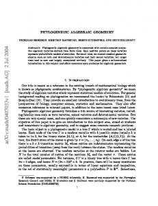
The interlacing and distributivity properties extend to bilattices in the obvious way: we say that a bilattice is interlaced (distributive) when its pre-bilattice reduct is interlaced (distributive). Figure 1.1 shows the double Hasse diagram of some of the most important pre-bilattices. The diagrams should be read as follows: a ≤t b if there is a path from a to b which goes uniformly from left to right, while a ≤k b if there is a path from a to b which goes uniformly from the bottom to the top3 . The four lattice operations are thus uniquely determined by the diagram, while negation, if there is one, corresponds to reflection along the vertical axis connecting ⊥ and >. It is then clear that all the pre-bilattices shown in Figure 1.1 can be endowed with a negation in a unique way, and so turned into bilattices. When no confusion is likely to arise, we shall use the same name to denote a particular pre-bilattice and its associated bilattice: the names used in the diagrams are by now more or less standard in the literature (SEVEN is sometimes called DEFAULT , which is the name originally used by Ginsberg [29], since this bilattice was introduced with applications to default logic in mind).

3

It is worth pointing out that, unlike lattices, not all finite bilattices can be represented in this way: for more on this, see the notions introduced by Avron [5] of “graphically representable” and “precisely representable” pre-bilattice.

12


The smallest non-trivial bilattice is FOUR. This algebra has a key role among bilattices, both from an algebraic and from a logical point of view, as we shall see. FOUR is distributive and, as a bilattice, it is a simple algebra. In fact it is, up to isomorphism, the only subdirectly irreducible bounded distributive bilattice (this is proved, for instance, in [36]). Let us also note that the {∧, ∨, ¬}-reduct of FOUR coincides with the fourelement De Morgan algebra that was used by Belnap [7] to define the Belnap-Dunn four-valued logic. In fact, we shall see that the logic of distributive bilattices (both with and without implication) turns out to be a conservative expansion of the Belnap-Dunn logic. Proposition 1.3.7 (De Morgan laws). The following equations hold in any bilattice: ¬(x ∧ y) ≈ ¬x ∨ ¬y ¬(x ⊗ y) ≈ ¬x ⊗ ¬y

¬(x ∨ y) ≈ ¬x ∧ ¬y ¬(x ⊕ y) ≈ ¬x ⊕ ¬y.

Moreover, if the bilattice is bounded, then ¬> = >, ¬⊥ = ⊥, ¬t = f and ¬f = t. So, if a bilattice B = hB, ∧, ∨, ⊗, ⊕, ¬i is distributive, or at least the truth lattice of B is distributive, then the reduct hB, ∧, ∨, ¬i is a De Morgan lattice. It is also easy to check that the four De Morgan laws imply that the negation operator satisfies (neg1) and (neg2). Then, it is obvious that the class of bilattices, denoted by BiLat, is equationally axiomatizable. Analogously to what we did in the case of pre-bilattices, we will denote by IntBiLat and DBiLat the classes of interlaced bilattices and distributive bilattices, which are also equationally axiomatizable. It is obvious that DBiLat ⊆ IntBiLat ⊆ BiLat, and these inclusions are all strict, as we shall see presently. Further expansions of the similarity type {∧, ∨, ⊗, ⊕, ¬}, which may be considered the standard bilattice language, have also been considered in the literature. Fitting [21], for instance, introduced a kind of dual negation operator, which he called conflation, and an implication-like connective called guard, while Arieli and Avron [3] investigated different choices for a bilattice implication. However, throughout this work we will always deal only with the basic language {∧, ∨, ⊗, ⊕, ¬}, except for the last two chapters, where we will consider the expansion obtained by adding one of Arieli and Avron’s implication connectives. An interesting class of (pre-)bilattices can be constructed as a kind of product of two lattices. We shall see that this construction, due to Fitting4 [18] has a natural intuitive interpretation, and gives rise to a class of structures that enjoys nice algebraic properties. 4

The essential of the definition are already in [29], but Ginsberg considered only a special case of the construction, what he called “world-based bilattices”.


13

Definition 1.3.8. Let L1 = hL1 , u1 , t1 i and L2 = hL2 , u2 , t2 i be two lattices with associated orders ≤1 and ≤2 . Then the product pre-bilattice L1 L2 = hL1 × L2 , ∧, ∨, ⊗, ⊕i is defined as follows. For all ha1 , a2 i , hb1 , b2 i ∈ L1 × L2 , ha1 , a2 i ∧ hb1 , b2 i = ha1 u1 b1 , ha1 , a2 i ∨ hb1 , b2 i = ha1 t1 b1 , ha1 , a2 i ⊗ hb1 , b2 i = ha1 u1 b1 , ha1 , a2 i ⊕ hb1 , b2 i = ha1 t1 b1 ,

a2 t2 b2 i a2 u2 b2 i a2 u2 b2 i a2 t2 b2 i .

It easy to check that the structure L1 L2 is always an interlaced pre-bilattice, and it is distributive if and only if both L1 and L2 are distributive. From the definition it is also obvious that ha1 , a2 i ≤k hb1 , b1 i

iff

a1 ≤1 b1 and a2 ≤2 b2

ha1 , a2 i ≤t hb1 , b1 i

iff

a1 ≤1 b1 and a2 ≥2 b2 .

and

The construction, as we have said, has a natural interpretation: we can think of the first component of each element of the form ha1 , a2 i as representing evidence for the truth of some sentence, while the second component can be thought of as representing the evidence against the truth (or for the falsity) of that sentence. It is not difficult to convince oneself that the truth lattice operations ∧ and ∨ act on each component according to our intuitions, as generalizations of classical conjunction and disjunction: for instance ∧ takes the infimum of the “truth component” and the supremum of the “falsity component”. More unusual, perhaps, are the two knowledge lattice connectives. As Fitting [20] puts it: If we think of ≤k as being an ordering by knowledge, then ⊗ is a consensus operator: p ⊗ q is the most that p and q can agree on. Likewise ⊕ is a ‘gullability’ operator: p ⊕ q accepts and combines the knowledge of p with that of q, whether or not there is a conflict. Loosely, it believes whatever it is told. If the two lattices L1 and L2 are isomorphic (so we may assume that they coincide, and denote both lattices just by L), then it is possible to define a negation in L L, so we speak of product bilattice instead of product pre-bilattice. Negation is defined as ¬ha1 , a2 i = ha2 , a1 i. Once again, it is easy to see that the behaviour of this operation is consistent with the intuitive interpretation we have proposed.

14


Using the construction we have described, we are now able to settle the question of whether the inclusions between the subvarieties of (pre-)bilattices mentioned above are strict. It is easy to see that FIVE and SEVEN are not interlaced, hence we have IntPreBiLat PreBiLat. To see that DPreBiLat IntPreBiLat it is enough to consider a product pre-bilattice L L where L is a non-distributive lattice. Since all the examples of pre-bilattices considered can be turned into bilattices, as an immediate consequence we also have DBiLat IntBiLat BiLat. Before proceeding, let us note that there is an important difference between the two variants of the construction described; this fact, although easily seen, has not received much attention in the literature on bilattices so far. The difference is that the product pre-bilattice construction can be regarded as a particular case of a direct product, while this is not the case for the product bilattice. As anticipated above, all lattices L = hL, u, ti can be seen as degenerated pre-bilattices in at least four different ways. We can consider the following four algebras: L++ L+− L−+ L−−

= hL, u, t, u, ti = hL, u, t, t, ui = hL, t, u, u, ti = hL, t, u, t, ui.

The first superscript, + or −, says whether we are taking as truth order the same order than in the original lattice or the dual one; and the second superscript refers to the same for the knowledge order. Using this notation, it is easy to see that the product pre-bilattice L1 L2 coincides with the direct product L++ 1 × −+ ++ −+ L2 . Notice also that L1 = hL1 , u1 , t1 , u1 , t1 i and L2 = hL2 , t2 , u2 , u2 , t2 i. In the next chapter we will come back to this construction, relating it to the representation theorem for unbounded pre-bilattices; for now it suffices to note that, of course, the product bilattice is not a direct product, because in general the factor lattice need not have a negation. We close this section stating the known representation theorem in its two versions: for bounded interlaced pre-bilattices and for bounded interlaced bilattices. This theorem has been stated and proved in several works, several versions, and different degrees of generality5 . The last and perhaps deeper work on it, and in general on interlaced bounded (pre-)bilattices, is Avron’s [6]. Theorem 1.3.9 (Representation, 1). Let B be a bounded pre-bilattice. The following statements are equivalent. (i) B is an interlaced pre-bilattice. (ii) There are two bounded lattices L1 and L2 such that B is isomorphic to L1 L2 . 5

For a brief review of these versions, see [36].


15

Although, as we have pointed out, many versions of the theorem are to be found in the literature, all of them use essentially the same proof strategy, of which we present here a sketch in order to help understand why this kind of proof does not work in the unbounded case. Of course, that (ii) implies (i) is immediate. To prove the other implication we need to construct L1 and L2 . This can be done by considering principal upsets and/or downsets of some of the bounds, together with the lattice operations inherited from the pre-bilattice. For this, having just one of the bounds is sufficient; of course, if we use ⊥ or >, then we have to consider upsets and downsets relative to the truth order, and similarly with t or f we need to use the knowledge order. Let us take, for instance, ⊥ and the order ≤t . Then we have L1 = h{a ∈ B : a ≥t ⊥}, ⊗, ⊕, ⊥, ti = h{a ∈ B : a ≥t ⊥}, ∧, ∨, ⊥, ti L2 = h{a ∈ B : a ≤t ⊥}, ⊗, ⊕, ⊥, fi = h{a ∈ B : a ≤t ⊥}, ∨, ∧, ⊥, fi. Taking a look at the Hasse diagrams in Figure 1.1, one may observe that, from a geometrical point of view, we are making a kind of projection of each point of the pre-bilattice on the two axes connecting ⊥ to t and ⊥ to f, fixing ⊥ as the origin. The isomorphism h : B → L1 × L2 is in this case defined as, for all a ∈ B, h(a) = ha ∨ ⊥, a ∧ ⊥i. Its inverse h−1 : L1 × L2 → B is defined as h−1 (ha1 , a2 i) = a1 ⊕ a2 . Injectivity of these maps is easily proved using Proposition 1.3.4 (1.2) and (1.3), which can be also used to give altenative decompositions, using the other bounds of the pre-bilattice. We stress that the key point here is that there is at least one bound (geometrically, a point which can be taken to be the origin of the axes on which we are making the projections). The representation theorem for bilattices is just a special case of the former: Theorem 1.3.10 (Representation, 2). Let B be a bounded bilattice. The following statements are equivalent. (i) B is an interlaced bilattice. (ii) There is a bounded lattice L such that B is isomorphic to L L. Everything works as in the case of pre-bilattices, but now we have that L1 and L2 are isomorphic via the map given by the negation operator. As a corollary of the representation theorem, we get a characterization of subdirectly irreducible bounded interlaced (pre-)bilattices (see for instance [36]).

16


We have that a bounded pre-bilattice L1 L2 is subdirectly irreducible if and only if L1 is a subdirectly irreducible lattice and L2 is trivial or viceversa, L2 is a subdirectly irreducible lattice and L1 is trivial. For bilattices, we have that L L is subdirectly irreducible if and only if L is a subdirectly irreducible lattice.

Chapter 2

Logical bilattices: the logic LB

2.1

Semantical and Gentzen-style presentations

In this chapter we will study the logic LB, introduced by Arieli and Avron [3], from the standpoint of Abstract Algebraic Logic. We start by giving a semantical presentation of LB, and then consider a sequent calculus that is complete with respect to this semantics. Our semantical presentation of LB differs from Arieli and Avron’s original one in that they use a whole class of matrices (called “logical bilattices”) to define their logic, while we will consider only FOUR. However, as we shall see, the two definitions have been proved to be equivalent. Recall that FOUR is the smallest non-trivial bilattice and its {∧, ∨, ¬}-reduct is a four-element De Morgan algebra which is known to generate the variety of De Morgan lattices. Indeed, as we have anticipated, the Belnap-Dunn four-valued logic is the logic defined by the logical matrix hM4 , Tri where M4 is this fourelement De Morgan algebra and Tr is the set {>, t} (see [23, Proposition 2.3]). According to the interpretation proposed by Belnap and Dunn, the elements of FOUR may be thought of as: only true (t), only false (f), both true and false (>), and neither true nor false (⊥). Thus, taking Tr = {>, t} as the set of designated elements corresponds to the intuitive idea of preferring those values which are at least true (but possibly also false). Arieli and Avron followed the same intuition when they introduced the logic LB. Let us give the formal definition: Definition 2.1.1. Let LB = hFm, LB i be the logic defined by the matrix hFOUR, Tri. As usual, the algebra Fm of formulas is the free algebra generated by a countable set Var of variables using the algebraic language {∧, ∨, ⊗, ⊕, ¬}. Note that we do not include constants in the language. By definition, for every set 17

Chapter 2. Logical bilattices: the logic LB

18

Axiom:

(Ax) Γ, ϕ B ϕ, ∆.

Rules:

Cut Rule plus the following logical rules:

(∧B)

Γ, ϕ, ψ B ∆ Γ, ϕ ∧ ψ B ∆ Γ, ¬ϕ B ∆ Γ, ¬ψ B ∆ Γ, ¬(ϕ ∧ ψ) B ∆

(¬ ∧ B)

(∨B)

Γ, ϕ B ∆ Γ, ψ B ∆ Γ, ϕ ∨ ψ B ∆ Γ, ¬ϕ, ¬ψ B ∆ Γ, ¬(ϕ ∨ ψ) B ∆

(¬ ∨ B)

(⊗B)

Γ, ϕ, ψ B ∆ Γ, ϕ ⊗ ψ B ∆

(¬ ⊗ B)

(⊕B)

Γ, ϕ B ∆ Γ, ψ B ∆ Γ, ϕ ⊕ ψ B ∆

(¬ ⊕ B)

(¬¬B)

Γ, ¬ϕ, ¬ψ B ∆ Γ, ¬(ϕ ⊗ ψ) B ∆

Γ, ¬ϕ B ∆ Γ, ¬ψ B ∆ Γ, ¬(ϕ ⊕ ψ) B ∆ Γ, ϕ B ∆ Γ, ¬¬ϕ B ∆

(B∧)

(B¬∧)

(B∨)

(B¬∨)

(B⊗)

(B¬⊗)

(B⊕)

Γ B ∆, ϕ Γ B ∆, ψ Γ B ∆, ϕ ∧ ψ Γ B ∆, ¬ϕ, ¬ψ Γ B ∆, ¬(ϕ ∧ ψ) Γ B ∆, ϕ, ψ Γ B ∆, ϕ ∨ ψ Γ B ∆, ¬ϕ Γ B ∆, ¬ψ Γ B ∆, ¬(ϕ ∨ ψ) Γ B ∆, ϕ Γ B ∆, ψ Γ B ∆, ϕ ⊗ ψ Γ B ∆, ¬ϕ Γ B ∆, ¬ψ Γ B ∆, ¬(ϕ ⊗ ψ) Γ B ∆, ϕ, ψ Γ B ∆, ϕ ⊕ ψ

(B¬⊕)

Γ B ∆, ¬ϕ, ¬ψ Γ B ∆, ¬(ϕ ⊕ ψ)

(B¬¬)

Γ B ∆, ϕ Γ B ∆, ¬¬ϕ

Table 2.1: A complete sequent calculus for the logic LB

2.1. Semantical and Gentzen-style presentations

19

Γ ∪ {ϕ} of formulas it holds that Γ LB ϕ if and only if, for every valuation h ∈ Hom(Fm, FOUR), if h[Γ] ⊆ Tr then h(ϕ) ∈ Tr. We will now remind two important results obtained in [3]. The first is the introduction of a complete axiomatization of LB by means of a sequent calculus1 . Here by sequent we mean a pair hΓ, ∆i where Γ and ∆ are both finite non-empty sets of formulas; to denote the sequent hΓ, ∆i we will usually write Γ B ∆ in order to avoid misunderstandings with other symbols that are sometimes used as sequent separator, such as ` , → or ⇒. The Gentzen system defined by the axiom and rules given in Table 2.1, that we call GLB , is the one introduced in [3] by Arieli and Avron2 . We will denote by |∼GLB the consequence relation determined on the set of sequents by this calculus, so {Γi B ∆i : i ∈ I} |∼GLB Γ B ∆ means that the sequent Γ B ∆ is derivable from the sequents {Γi B ∆i : i ∈ I}. By this we mean that there is a finite sequence Σ = S1 , . . . Sn of sequents such that Sn = Γ B ∆ and, for each Sm ∈ Σ, either Sm is an instance of (Ax) or Sm ∈ {Γi B ∆i : i ∈ I} or there are Sj , Sk ∈ Σ such that j, k < m and Sm has been obtained from Sj and Sk by the application of a rule of GLB . Since both the left- and right-hand side of our sequents are (finite) sets of formulas, rather than multisets or sequences, it is not necessary to include the structural rules of contraction and exchange; they are, so to speak, built-in in the formalism. Note also that, using (Ax), V Cut, (∧B) W and (B∨), it is easy to prove that the sequent Γ B ∆ is equivalent to Γ B ∆. Taking this into account, we may obtain formal proofs of the rules of left weakening (W B) and right weakening (BW ), as follows: V (Cut)

(Ax) VΓ B ∆ W W W ΓB ∆ ∆ B ∆, ϕ V W (Cut) Γ B ∆, ϕ Γ B ∆, ϕ

(Ax) V VΓ B ∆ W Γ, ϕ B Γ ΓB ∆ V W Γ, ϕ B ∆ Γ, ϕ B ∆

Hence, GLB has all the structural rules. In [3] it is proved that this calculus admits Cut Elimination (i.e., the Cut Rule is admissible) and is complete with respect to the semantics of LB, in the following sense: Theorem 2.1.2. The sequent calculus GLB is complete with respect to LB . That is, for any Γ ∪ {ϕ} ⊆ F m, we have Γ LB ϕ 1

iff

∅ |∼GLB Γ B ϕ.

An alternative sequent calculus, also complete w.r.t. the semantics of LB, was introduced in [33]. 2 Note that, unlike Arieli and Avron’s, our presentation requires that both sides of sequents be non-empty. However, it is straightforward to see that the two presentations generate essentially the same consequence relation.


20

The previous result can also be expressed saying that the Gentzen system GLB is adequate for the logic LB. The second important result we want to cite from [3], which justifies why LB is called the logic of logical bilattices, shows that the consequence relation LB may be defined using many other logical matrices instead of hFOUR, Tri. In order to state it, we need the following: Definition 2.1.3. A logical bilattice is a pair hB, F i where B is a bilattice and F is a prime bifilter of B. It is obvious that logical bilattices are also matrices in the sense of AAL: so each logical bilattice determines a logic. Note also that, since FOUR has (only) one proper bifilter, hFOUR, Tri is a logical bilattice, namely the one we used to introduce LB. A key result of [3] is then that all logical bilattices define the same consequence relation (i.e. LB ): Theorem 2.1.4. If hB, F i is a logical bilattice then the logic determined by the matrix hB, F i coincides with LB. That is, for every set Γ ∪ {ϕ} of formulas it holds that Γ LB ϕ iff Γ |=hB,F i ϕ. This last theorem is indeed a straightforward consequence of the following lemma (see [3, Theorem 2.17]). Lemma 2.1.5. Let B be a bilattice and let F ( B. Then the following statements are equivalent: (i) F is a prime bifilter of B, (ii) there is a unique epimorphism πF : B −→ FOUR such that F = πF−1 [Tr], (iii) there is an epimorphism πF : B −→ FOUR such that F = πF−1 [Tr]. We stress that the epimorhism πF is the map defined, for all a ∈ B, by  > if a ∈ F and ¬a ∈ F    t if a ∈ F and ¬a 6∈ F πF (a) := f if a 6∈ F and ¬a ∈ F    ⊥ if a 6∈ F and ¬a 6∈ F Theorem 2.1.4 justifies the claim that the logic of logical bilattices is indeed the logic of the matrix hFOUR, Tri. In Section 2.4 we will see that, from an algebraic point of view, the logic LB may be also considered in some sense as the logic of distributive bilattices.

2.2. Hilbert-style presentation

2.2

21

Hilbert-style presentation

In the literature a Hilbert-style presentation for the logic LB has not yet been given. The aim of this section is to fill this gap, introducing a strongly complete Hilbert-style calculus for this logic. It is well known that, from a proof theoretic point of view, sequent calculi (especially those enjoying cut elimination and the subformula property) are better suited for searching proofs than Hilbert-style calculi. However, from the point of view of AAL, having a Hilbert-style presentation provides a lot of benefits, since it allows to characterize on any algebra the filters of the logic (i.e. those sets of elements of the algebra that are closed under the rules of the logic). This kind of considerations, besides its intrinsic interest, motivated the introduction of our calculus. From the semantical definition of LB, is it obvious that this logic is a conservative expansion of the Belnap-Dunn four-valued logic. This observation suggests that, in order to find a Hilbert-style presentation for LB, we can just expand any axiomatization of the Belnap-Dunn logic. We shall consider the one given by Font in [23], which consists of the first fifteen rules of Table 2.2. Note that, like Font’s, our calculus has no axioms: this is due to the fact that LB has no theorems, just like the Belnap-Dunn logic. To see this, it is sufficient to observe that {⊥} is a subalgebra of FOUR and ⊥ is not a designated element in the matrix hFOUR, Tri. Let us stress that here it is crucial that we do not have any of the constants {>, t, f} in the language. Hence, all Hilbert-style presentations for LB must be free of axioms and consist only of (proper) rules. Of course, as noted by Font [23], and contrary to what is claimed in [3, p. 37], this absence of theorems does not mean that there may not be Hilbert-style presentations for LB. Let us introduce formally the consequence relation determined by our rules: Definition 2.2.1. The logic `H is the consequence relation defined through the rules of Table 2.2. The closure operator associated with `H will be denoted CH . We shall devote the rest of the section to prove that this calculus is strongly complete with respect to the semantics of LB. The strategy of our proof is very similar to the one used in [23] for the Belnap-Dunn logic, and is based on a normal form representation of formulas. First of all, let us verify that `H is sound: Proposition 2.2.2 (Soundness). Given a set of formulas Γ ⊆ F m and a formula ϕ ∈ F m, if Γ `H ϕ, then Γ LB ϕ. Proof. It is sufficient to check that in FOUR the set Tr is closed w.r.t. all rules given in Table 2.2. In the following propositions (from 2.2.3 to 2.2.8) we state some lemmas that will be needed to prove our normal form theorem (Theorem 2.2.9).


22

(R1)

p∧q p

(R2)

p (R4) p ∨ q p ∨ (q ∨ r) (p ∨ q) ∨ r

(R7)

p∨r (R10) ¬¬p ∨ r (R13)

(¬p ∧ ¬q) ∨ r ¬(p ∨ q) ∨ r

p∨q (R5) q ∨ p (R8)

p ∨ (q ∧ r) (p ∨ q) ∧ (p ∨ r)

(R14)

(R6) (R9)

p∨p p

(p ∨ q) ∧ (p ∨ r) p ∨ (q ∧ r)

¬¬p ∨ r p∨r

(R12)

¬(p ∨ q) ∨ r (¬p ∧ ¬q) ∨ r

¬(p ∧ q) ∨ r (¬p ∨ ¬q) ∨ r

(R15)

(¬p ∨ ¬q) ∨ r ¬(p ∧ q) ∨ r

(R11)

(R16)

(p ⊗ q) ∨ r (p ∧ q) ∨ r

(R19)

(p ∨ q) ∨ r (p ⊕ q) ∨ r

(R20)

(¬p ⊗ ¬q) ∨ r ¬(p ⊗ q) ∨ r

(¬p ⊕ ¬q) ∨ r ¬(p ⊕ q) ∨ r

(R23)

¬(p ⊕ q) ∨ r (¬p ⊕ ¬q) ∨ r

(R22)

p q (R3) p ∧ q

p∧q q

(R17)

(p ∧ q) ∨ r (p ⊗ q) ∨ r

(R18)

(R21)

(p ⊕ q) ∨ r (p ∨ q) ∨ r

¬(p ⊗ q) ∨ r (¬p ⊗ ¬q) ∨ r

Table 2.2: A complete Hilbert-style calculus for the logic LB Proposition 2.2.3. The following rules follow from (R1) to (R23): ϕ ϕ∨r for each one of the rules (Ri) , ψ ψ∨r where i ∈ {10, . . . , 23}.

(i) The rule (Ri+ )

(ii) The rule

ϕ∧r in the same cases. ψ∧r

Proof. (i) From ϕ by (R4) we obtain ϕ ∨ ψ. Then we apply (Ri ) to obtain ψ ∨ ψ and by (R6) we have ψ. (ii) From ϕ ∧ r by (R1) we obtain ϕ. Now using (i) we obtain ψ. Also from ϕ ∧ r, by (R2), follows r. Thus applying (R3) we obtain ψ ∧ r. The following properties are also easily proved (we omit the proof):


23

Proposition 2.2.4. From (R1), . . . , (R9) and (R16+ ), . . . , (R19+ ) we can derive the following rules: (R1’)

p⊗q p

(R2’)

p⊗q q

(R3’)

p q p⊗q

(R4’)

p p⊕q

(R5’)

p⊕q q⊕p

(R6’)

p⊕p p

(R7’)

p ⊕ (q ⊕ r) (p ⊕ q) ⊕ r

(R8’)

p ⊕ (q ⊗ r) (p ⊕ q) ⊗ (p ⊕ r)

(R9’)

(p ⊕ q) ⊗ (p ⊕ r) p ⊕ (q ⊗ r)

Proposition 2.2.5. The interderivability relation a`H is a congruence w.r.t. the operations ∧ and ∨. Proof. It is sufficient to show that the following two rules p∧r q∧r (p ∧ q) ∧ r

p∨r q∨r (p ∧ q) ∨ r

together with the rules ϕ∨r ψ∨r

and

ϕ∧r ψ∧r

ϕ in Table 2.2) are all derivable in `H . For the rules in Taψ ble 2.2 that belong to the {∧, ∨}-fragment, it is known that they follow just from rules (R1) to (R9). And for (R10) to (R23) the conjunction case is shown by Proposition 2.2.3 (ii), while the disjunction case can be easily shown by using the associativity of ∨. Then we know that ϕ `H ψ implies ϕ ∧ γ `H ψ ∧ γ and ϕ ∨ γ `H ψ ∨ γ for any γ ∈ F m. So, assuming ϕ1 `H ψ1 and ϕ2 `H ψ2 , from the former we obtain ϕ1 ∧ ϕ2 `H ψ1 ∧ ϕ2 and from the latter ψ1 ∧ ϕ2 `H ψ1 ∧ ψ2 . Hence ϕ1 ∧ϕ2 `H ψ1 ∧ψ2 . By symmetry, we may conclude that ϕ1 a`H ψ1 and ϕ2 a`H ψ2 imply ϕ1 ∧ϕ2 a`H ψ1 ∧ψ2 . A similar reasoning shows that a`H is also a congruence w.r.t. ∨. (for each rule

Definition 2.2.6. Lit = Var ∪ {¬p : p ∈ Var} is the set of literals. Cl, the set of clauses, is the least set containing Lit and closed under ∨. For any ϕ ∈ F m, the set var (ϕ) of variables of ϕ is defined in the usual way. For Γ ⊆ F m, we set var (Γ) =

[ ϕ∈Γ

var (ϕ) .


24

For any ϕ ∈ Cl, the set lit (ϕ) of literals of ϕ is defined inductively by lit (ϕ) = {ϕ} if ϕ ∈ Lit and lit (ϕ ∨ ψ) = lit (ϕ) ∪ lit (ψ). For Γ ⊆ Cl, we set [ lit (Γ) = lit (ϕ) . ϕ∈Γ

Proposition 2.2.7. For all ϕ ∈ F m, there is a finite Γϕ ⊆ Cl such that var (ϕ) = var (Γ) and for every ψ ∈ F m, CH (ϕ ∨ ψ) = CH ({γ ∨ ψ : γ ∈ Γ}) . Proof. By induction on the length of ϕ. If ϕ = p ∈ Var, then Γϕ = {p}. If ϕ = ϕ1 ∧ ϕ2 and by inductive hypothesis Γϕ1 , Γϕ2 correspond respectively to ϕ1 and ϕ2 , then we may take Γϕ = Γϕ1 ∪ Γϕ2 and we have var (ϕ) = var (Γϕ ). We also have CH (ϕ ∨ ψ) = = = = = = =

CH ((ϕ1 ∧ ϕ2 ) ∨ ψ) CH ((ϕ1 ∨ ψ) ∧ (ϕ2 ∨ ψ)) CH (ϕ1 ∨ ψ, ϕ2 ∨ ψ) by (R1), (R2), (R3) CH (CH (ϕ1 ∨ ψ) ∪ CH (ϕ2 ∨ ψ)) CH (CH ({γ1 ∨ ψ : γ1 ∈ Γϕ1 }) ∪ CH ({γ2 ∨ ψ : γ2 ∈ Γϕ2 })) CH ({γ ∨ ψ : γ ∈ Γϕ }) .

If ϕ = ϕ1 ∨ ϕ2 and Γϕ1 , Γϕ2 correspond respectively to ϕ1 and ϕ2 , then we take Γϕ = {γ1 ∨ γ2 : γ1 ∈ Γϕ1 , γ2 ∈ Γϕ2 } and we have var (ϕ) = var (Γϕ ). We also have: CH (ϕ ∨ ψ) = = = = = = =

CH ((ϕ1 ∨ ϕ2 ) ∨ ψ) CH (ϕ1 ∨ (ϕ2 ∨ ψ)) (by inductive hypothesis) CH ({γ1 ∨ (ϕ2 ∨ ψ) : γ1 ∈ Γϕ1 }) CH ({ϕ2 ∨ (γ1 ∨ ψ) : γ1 ∈ Γϕ1 }) CH ({γ2 ∨ (γ1 ∨ ψ) : γ1 ∈ Γϕ1 , γ2 ∈ Γϕ2 }) CH ({(γ1 ∨ γ2 ) ∨ ψ : γ1 ∈ Γϕ1 , γ2 ∈ Γϕ2 }) .

If ϕ = ϕ1 ⊗ ϕ2 , then CH (ϕ ∨ ψ) = CH ((ϕ1 ⊗ ϕ2 ) ∨ ψ). By (R16) and (R17) we have CH ((ϕ1 ⊗ ϕ2 ) ∨ ψ) = CH ((ϕ1 ∧ ϕ2 ) ∨ ψ) . So we may apply the procedure for ϕ = ϕ1 ∧ ϕ2 .


25

If ϕ = ϕ1 ⊕ ϕ2 , then CH (ϕ ∨ ψ) = CH ((ϕ1 ⊕ ϕ2 ) ∨ ψ) . By (R18) and (R19) we have CH ((ϕ1 ⊕ ϕ2 ) ∨ ψ) = CH ((ϕ1 ∨ ϕ2 ) ∨ ψ) . So we may apply the procedure for ϕ = ϕ1 ∨ ϕ2 . If ϕ = ¬ϕ0 , then we have to distinguish several cases on ϕ0 . If ϕ0 = p ∈ Var, then ϕ ∈ Lit ⊆ Cl, so we may take Γϕ = {ϕ}. If ϕ0 = ¬ϕ00 , then ϕ = ¬¬ϕ00 and by (R10) and (R11) we have CH (ϕ ∨ ψ) = CH (ϕ00 ∨ ψ) . Now just note that ϕ00 is shorter that ϕ and its corresponding set Γϕ also works for ϕ. If ϕ0 = ϕ1 ∧ ϕ2 , then ϕ = ¬ (ϕ1 ∧ ϕ2 ) and by (R14) and (R15) we have CH (ϕ ∨ ψ) = CH ((¬ϕ1 ∨ ¬ϕ2 ) ∨ ψ) . Both ¬ϕ1 and ¬ϕ2 are shorter than ¬ (ϕ1 ∧ ϕ2 ), so the same procedure for the case of ϕ = ϕ1 ∨ ϕ2 works. If ϕ0 = ϕ1 ∨ ϕ2 , then ϕ = ¬ (ϕ1 ∨ ϕ2 ) and by (R12) and (R13) we have CH (ϕ ∨ ψ) = CH ((¬ϕ1 ∧ ¬ϕ2 ) ∨ ψ) . Both ¬ϕ1 and ¬ϕ2 are shorter than ¬ (ϕ1 ∨ ϕ2 ), so the same procedure for the case of ϕ = ϕ1 ∧ ϕ2 works. If ϕ0 = ϕ1 ⊗ ϕ2 , then ϕ = ¬ (ϕ1 ⊗ ϕ2 ) and by (R20) and (R21) we have CH (ϕ ∨ ψ) = CH ((¬ϕ1 ⊗ ¬ϕ2 ) ∨ ψ) . Both ¬ϕ1 and ¬ϕ2 are shorter than ¬ (ϕ1 ⊗ ϕ2 ), hence the procedure applied for ϕ = ϕ1 ⊗ ϕ2 works. If ϕ0 = ϕ1 ⊕ ϕ2 , then ϕ = ¬ (ϕ1 ⊕ ϕ2 ) and by (R22) and (R23) we have CH (ϕ ∨ ψ) = CH ((¬ϕ1 ⊕ ¬ϕ2 ) ∨ ψ) . Both ¬ϕ1 and ¬ϕ2 are shorter than ¬ (ϕ1 ⊕ ϕ2 ). Once again, the procedure applied for ϕ = ϕ1 ⊕ ϕ2 works.

26


Proposition 2.2.8. For all ϕ ∈ F m there is a finite Γϕ ⊆ Cl such that var (ϕ) = var (Γϕ ) and CH (ϕ) = CH (Γϕ ) . Proof. By induction on the length of ϕ. If ϕ = p ∈ Var, then take Γϕ = {ϕ}. If ϕ = ϕ1 ∧ ϕ2 by (R1), (R2) and (R3) we have CH (ϕ) = CH (ϕ1 , ϕ2 ). So we may take Γϕ = Γϕ1 ∪ Γϕ2 and we are done. If ϕ = ϕ1 ∨ ϕ2 then by Proposition 2.2.7 and (R5) we have: CH (ϕ) = CH ({γ1 ∨ ϕ2 : γ1 ∈ Γϕ1 }) = CH ({ϕ2 ∨ γ1 : γ1 ∈ Γϕ1 }) = CH ({γ2 ∨ γ1 : γ1 ∈ Γϕ1 , γ2 ∈ Γϕ2 }) . Since Γϕ1 , Γϕ2 ⊆ Cl are finite, Γϕ = {γ1 ∨ γ2 : γ1 ∈ Γϕ1 , γ2 ∈ Γϕ2 } ⊆ Cl is also finite and we are done. If ϕ = ϕ1 ⊗ ϕ2 , by (R16+ ) and (R17+ ) we have CH (ϕ) = CH (ϕ1 , ϕ2 ), so we may take Γϕ = Γϕ1 ∪ Γϕ2 and we are done. If ϕ = ϕ1 ⊕ϕ2 , since by (R18+ ) and (R19+ ) we have CH (ϕ1 ⊕ ϕ2 ) = CH (ϕ1 ∨ ϕ2 ), we may apply the procedure for ϕ = ϕ1 ∨ ϕ2 . If ϕ = ¬ϕ0 we have to distinguish several cases. If ϕ0 = p ∈ Var, then ϕ ∈ Cl, so we may take Γϕ = {ϕ}. If ϕ0 = ¬ϕ00 , then by (R10+ ) and (R11+ ) we have CH (ϕ) = CH (ϕ00 ) and since ϕ00 is shorter that ϕ we are done. If ϕ0 = ϕ1 ∧ ϕ2 then by (R14+ ) and (R15+ ) we have CH (ϕ) = CH (¬ϕ1 ∨ ¬ϕ2 ), so we may apply the procedure for the ∨-disjunction case. If ϕ0 = ϕ1 ∨ ϕ2 then by (R12+ ) and (R13+ ) we have CH (ϕ) = CH (¬ϕ1 , ¬ϕ2 ), so applying the inductive hypothesis we are done. If ϕ0 = ϕ1 ⊗ ϕ2 , then ϕ = ¬ (ϕ1 ⊗ ϕ2 ) and by (R20+ ) and (R21+ ) we have CH (ϕ) = CH (¬ϕ1 ⊗ ¬ϕ2 ), so the procedure applied for the ⊗-conjunction works. If ϕ0 = ϕ1 ⊕ ϕ2 , then ϕ = ¬ (ϕ1 ⊕ ϕ2 ) and by (R22+ ) and (R23+ ) we have CH (ϕ) = CH (¬ϕ1 ⊕ ¬ϕ2 ), so the procedure applied for the ⊕-disjunction works.

Theorem 2.2.9 (Normal Form). Every formula is equivalent, both through a`H and =||=LB , to a ∧-conjunction of clauses with the same variables.


27

V V Proof. By Proposition 2.2.8 we have that ϕ a`H Γϕ , where Γϕ is any conjunction of all the clauses in Γϕ . Now, by Proposition 2.2.2, this implies also that V Γϕ =||=LB ϕ. The following lemma will allow us to prove the completeness of our Hilbert calculus. Lemma 2.2.10. For all Γ ⊆ Cl and ϕ ∈ Cl, the following are equivalent: (i) Γ `H ϕ, (ii) Γ LB ϕ, (iii) ∃γ ∈ Γ such that lit (γ) ⊆ lit (ϕ), (iv) ∃γ ∈ Γ such that γ `H ϕ. Proof. (i) ⇒ (ii) follows from Proposition 2.2.2. (ii) ⇒ (iii). For a fixed ϕ ∈ Cl, define a homomorphism h : Fm → FOUR as follows. For every p ∈ Var:  t    > h (p) = ⊥    f

if if if if

p∈ / lit (ϕ) and ¬p ∈ lit (ϕ) p, ¬p ∈ / lit (ϕ) p, ¬p ∈ lit (ϕ) p ∈ lit (ϕ) and ¬p ∈ / lit (ϕ)

If p ∈ lit (ϕ), then h (p) ∈ {f, ⊥} and also h (¬p) ∈ {f, ⊥} when ¬p ∈ lit (ϕ). Since f ≤t ⊥, we have h (ϕ) ∈ {f, ⊥}. Suppose (iii) fails: then for any γ ∈ Γ there would be ψγ ∈ lit (γ) such that ψγ ∈ / lit (ϕ). Then we would have h (ψγ ) ∈ {t, >} and as a consequence h (γ) ∈ {t, >}. Thus we would have, against (ii), h [Γ] ⊆ {t, >} while h (ϕ) ∈ / {t, >}. (iii) ⇒ (iv). If lit (γ) ⊆ lit (ϕ) and γ, ϕ ∈ Cl, then ϕ is a disjunction of the same literals appearing in γ plus other ones, modulo some associations, permutations etc. Therefore, applying rules (R4) to (R7) and repeatedly using Proposition 2.2.5, we obtain γ `H ϕ. (iv) ⇒ (i). Immediate. Theorem 2.2.11 (Completeness). For all Γ ⊆ F m and ϕ ∈ F m, it holds that Γ LB ϕ iff Γ `H ϕ. Proof. By Lemma 2.2.10 and Theorem 2.2.9.

28

2.3


Tarski-style characterizations

With the help of the Hilbert calculus introduced in the previous section, we will now investigate our logic from the point of view of Abstract Algebraic Logic. In particular, we study the algebraic models and g-models of LB, characterize the classes AlgLB and Alg∗ LB and compare them with the class of algebraic reducts of logical bilattices, which we will denote by LoBiLat. We will also prove that the Gentzen calculus introduced in Section 2.1 is algebraizable and individuate its equivalent algebraic semantics. Let us start by checking that LB has no consistent extensions. We shall need the following: Lemma 2.3.1. Let hB, F i be a matrix such that B is a distributive bilattice and F is a proper and non-empty bifilter of B, i.e. ∅ = 6 F B. Then the logic defined by hB, F i is weaker than LB. Proof. Reasoning by contraposition, we will prove that Γ 2LB ϕ implies Γ 2hB,F i ϕ for all Γ ∪ {ϕ} ⊆ F m. In order to do this, it will be enough to show that hFOUR, Tri is a submatrix of any matrix of the form hB, F i. By assumption F is proper and non-empty, so there are a, b ∈ B such that a ∈ / F and b ∈ F . Let us denote by ⊥(a, b) the element a⊗b⊗¬a⊗¬b. Similarly, let >(a, b) = a⊕b⊕¬a⊕¬b, t(a, b) = ⊥(a, b) ∨ >(a, b) and f(a, b) = ⊥(a, b) ∧ >(a, b). Since F is a bifilter, from the assumptions it follows that >(a, b), t(a, b) ∈ F and ⊥(a, b), f(a, b) ∈ / F . It is easy to check that FOUR is embeddable into B via the map f defined as f (x) = x(a, b) for all x ∈ {⊥, >, t, f}. Moreover, Tr = f −1 [F ]. So if h : Fm −→ FOUR is a homomorphism such that h[Γ] ⊆ Tr but h(ϕ) ∈ / Tr, then also f [h[Γ]] ⊆ F but f (h(ϕ)) ∈ / F . Recalling that LB is the logic defined by the matrix hFOUR, Tri, we may then conclude that Γ 2LB ϕ implies Γ 2hB,F i ϕ. Let us say that a logic L = hFm, `L i is consistent if there exist ϕ, ψ ∈ F m such that ϕ 0L ψ. Then the previous lemma allows to obtain the following: Proposition 2.3.2. If a logic L = hFm, `L i is a consistent extension of LB, then `L = LB . Proof. By [25, Proposition 2.27], we know that any reduced matrix for L is of the form hB, F i, where B is a distributive bilattice and F is a bifilter. By the assumption of consistency, we may assume that there is at least one reduced matrix for L such that F is proper and non-empty. By Lemma 2.3.1, we know that the logic defined by such a matrix is weaker than LB; this implies that the class of all reduced matrices for L defines a weaker logic than LB. Since any logic is complete with respect to the class of its reduced matrices (see [46]), we may conclude that L itself is weaker than LB, so they must be equal.

2.3. Tarski-style characterizations

29

The two completeness results stated in the previous section allow us to give a characterization of LB in terms of some metalogical properties which are sometimes called Tarski-style conditions. In particular, we shall consider the following: the Property of Conjunction (PC) w.r.t. both conjunctions ∧ and ⊗, the Property of Disjunction (PD) w.r.t. both disjunctions ∨ and ⊕, the Property of Double Negation (PDN) and the Properties of De Morgan (PDM). Let us denote the closure operator associated with our logic by CLB . Then we may state the following: Proposition 2.3.3. The logic LB = hFm, CLB i satisfies the following properties: for all Γ ∪ {ϕ, ψ} ⊆ F m, (PC)

CLB (ϕ ∧ ψ) = CLB (ϕ ⊗ ψ) = CLB (ϕ, ψ)

(PDI)

CLB (Γ, ϕ ∨ ψ) = CLB (Γ, ϕ ⊕ ψ) = CLB (Γ, ϕ) ∩ CLB (Γ, ψ)

(PDN)

CLB (ϕ) = CLB (¬¬ϕ)

(PDM) CLB (¬(ϕ ∧ ψ)) = CLB (¬ϕ ∨ ¬ψ)) CLB (¬(ϕ ∨ ψ)) = CLB (¬ϕ ∧ ¬ψ)) CLB (¬(ϕ ⊗ ψ)) = CLB (¬ϕ ⊗ ¬ψ)) CLB (¬(ϕ ⊕ ψ)) = CLB (¬ϕ ⊕ ¬ψ)). Moreover, LB is the only consistent logic satisfying them. Proof. In [38, Theorem 4.1] it is proved that the Belnap-Dunn logic is the least logic satisfying all the above properties except those involving ⊗ and ⊕. Since our logic is a conservative expansion of the Belnap-Dunn, we need only to check that LB satisfies the conditions where ⊗ or ⊕ appears. (PC) is easily proved using the derivable rules (R16+ ) and (R17+ ) of our Hilbert calculus (see the first item of Proposition 2.2.3). Recalling that LB is finitary, to prove (PDI) we may use (PC), (R18+ ) and (R19+ ). Finally, the last two equalities of (PDM) are easily proved using rules from (R20+ ) to (R23+ ). Hence LB satisfies all the above properties. Moreover, it is the weakest one that satisfies them. In fact, any logic L = hFm, `L i satisfying the same properties will be closed under the rules of the Gentzen calculus GLB , which is complete w.r.t. the semantics of LB. So any derivation in GLB will produce only sequents which are derivable in L. Hence, by completeness, if Γ LB ϕ, then Γ `L ϕ. Now, applying Lemma 2.3.1, we may conclude that `L = LB . Another interesting feature of LB is the variable sharing property (VSP), that can be formulated as follows: if ϕ LB ψ, then var(ϕ) ∩ var(ψ) 6= ∅. Note that any logic L = hFm, `L i satisfying the (VSP) will be consistent, for it will hold that p 0L q for any two distinct propositional variables p and q. So from the


30

v >@

du

@ @

fv @

@ @

@v⊥

@vt

f

> u@

@ue @

@ @uc u @ut @ @ @u @u a@ b @u⊥

FOUR

N IN E

> t@ @ @tt B@ B @tc @tb a Bt @ @ @t⊥

f tB@

SEVEN

Figure 2.1: Some bilattices

previous result it also follows that LB is the only logic satisfying (PC), (PDI), (PDN), (PDM) and (VSP).

2.4

AAL study of LB

Let us now classify our logic according to some of the criteria of Abstract Algebraic Logic. Recall that, in the context of AAL, a logic L is said to be protoalgebraic if and only if, on any algebra, the Leibniz operator is monotone on the L-filters (this is not the original definition, but a characterization that has by now become standard; see, for instance, [10]). A logic is said to be selfextensional when the interderivability relation is a congruence of the formula algebra. The following proposition shows that our logic falls outside of both these categories: Proposition 2.4.1. The logic LB is non–protoalgebraic and non–selfextensional. Proof. Consider the bilattice N IN E, repeated in Figure 2.1. The only proper and non–empty LB–filters on N IN E are F1 = {e, >, t} ⊆ {b, c, d, e, >, t} = F2 . It is easy to check that ht, ei ∈ Ω hN IN E, F1 i but, because of negation, we have ht, ei ∈ / Ω hN IN E, F2 i. Hence, the Leibniz operator is not monotone on LB-filters. As to the second claim, note that for any p, q ∈ F m we have p ⊕ q =||=LB p ∨ q, but we can easily check that we do not have ¬ (p ⊕ q) =||=LB ¬ (p ∨ q). For instance in FOUR we have ¬ (t ⊕ >) = > ∈ {t, >} but ¬ (t ∨ >) = f ∈ / {t, >}. The fact that LB is not selfextensional constitutes one of the main difficulties of the AAL approach to it. As we have seen, this is due to the behaviour of the negation operator, and it is possible to see that this exception to selfextensionality is essentially the only one. We need the following lemmas. Lemma 2.4.2. Let ϕ, ψ ∈ F m be two formulas. The following statements are equivalent:

2.4. AAL study of LB

31

(i) FOUR ϕ ∧ (ϕ ⊗ ψ) ≈ ϕ (ii) ϕ `H ψ. Proof. (i) ⇒ (ii). Let h : Fm → FOUR be a homomorphism. If h(ϕ) = t, then t ⊗ h(ψ) = t, i.e. h(ψ) ≥k t, therefore h(ψ) ∈ {>, t}. If h(ϕ) = >, then > ∧ h(ψ) = >, i.e. h(ψ) ≥t >, hence h(ψ) ∈ {>, t}. (ii) ⇒ (i). Let h : Fm → FOUR be a homomorphism and assume that ϕ `H ψ. If h(ϕ) = t, then h(ψ) ∈ {>, t}, so h(ψ) ≥k h(ϕ). Hence h(ϕ)∧(h(ϕ)⊗h(ψ)) = h(ϕ) ∧ h(ϕ) = h(ϕ). If h(ϕ) = >, then h(ψ) ∈ {>, t}, so h(ψ) ≥t h(ϕ) and obviously h(ϕ) ≥k h(ψ). Hence we have h(ϕ) ∧ (h(ϕ) ⊗ h(ψ)) = h(ϕ) ∧ h(ψ) = h(ϕ). If h(ϕ) = ⊥, then h(ϕ) ∧ (h(ϕ) ⊗ h(ψ)) = ⊥ ∧ ⊥ = ⊥ = h(ϕ). Finally, the case where h(ϕ) = f is immediate. As an immediate consequence of the preceding result, we have the following: Lemma 2.4.3. Let ϕ, ψ ∈ F m be two formulas. The following statements are equivalent: (i) FOUR ϕ ≈ ψ, (ii) ϕ a`H ψ and ¬ϕ a`H ¬ψ. Proof. The only non-trivial implication is (ii)⇒(i). By Lemma 2.4.2, (ii) implies that in FOUR the following equations hold: ϕ ≈ ϕ ∧ (ϕ ⊗ ψ) ψ ≈ ψ ∧ (ϕ ⊗ ψ) ¬ψ ≈ ¬ψ ∧ (¬ϕ ⊗ ¬ψ) ¬ϕ ≈ ¬ϕ ∧ (¬ϕ ⊗ ¬ψ).

(2.1) (2.2) (2.3) (2.4)

Negating both sides of 2.3 and using De Morgan’s laws, we obtain ¬¬ψ ≈ ψ ≈ ¬(¬ψ ∧ (¬ϕ ⊗ ¬ψ)) ≈ ¬¬ψ ∨ ¬(¬ϕ ⊗ ¬ψ) ≈ ψ ∨ (¬¬ϕ ⊗ ¬¬ψ) ≈ ψ ∨ (ϕ ⊗ ψ). From this and 2.2 it follows that ψ ≈ ϕ ⊗ ψ. A similar reasoning shows that 2.1 and 2.4 imply ϕ ≈ ϕ ⊗ ψ. Hence ϕ ≈ ψ. The preceding result enables us to characterize the Tarski congruence associated with LB as the relation defined by the equations valid in FOUR:

32


Theorem 2.4.4. The Tarski congruence associated with LB = hFm, LB i is e Ω(LB) = {hϕ, ψi : FOUR ϕ ≈ ψ}. Proof. Obviously, the relation {hϕ, ψi : FOUR ϕ ≈ ψ} is a congruence and, by Lemma 2.4.3 (ii), it is also clear that it is the maximal congruence below the Frege relation. Recalling [25, Propositions 1.23 and 2.26], we can conclude that both Alg∗ LB and AlgLB are classes of algebras generating the same variety as FOUR (which is, as we have seen in Chapter ??, the variety DBiLat of distributive bilattices). In fact, we have the following: Theorem 2.4.5. The class AlgLB is the variety generated by FOUR, i.e. the variety of distributive bilattices. Proof. It is clear that FOUR ∈ Alg∗ LB ⊆ AlgLB. By [25, Theorem 2.23] we also have FOUR ∈ AlgLB = Ps (Alg∗ LB) ⊆ V (FOUR). Recall that V (FOUR) = DBiLat is congruence-distributive. Hence we may apply Jónsson’s Lemma [12, Corollary IV.6.10] to conclude that the subdirectly irreducible members of V (FOUR) belong to HS(FOUR), and clearly the only algebras in HS(FOUR) are the trivial one and FOUR itself. Then we may conclude that V (FOUR) = Ps (FOUR) ⊆ Ps (Alg∗ LB). Hence we obtain Ps (Alg∗ LB) = AlgLB = V (FOUR). An immediate corollary of the previous result concerning the algebraic reducts of logical bilattices is that LoBiLat * AlgLB. This is so because hSEVEN , {>, t}i is a logical bilattice, but SEVEN ∈ / AlgLB, for this bilattice is not distributive (not even interlaced, as one can easily see by cardinality condiderations). We can also verify that N IN E ∈ AlgLB, since this bilattice is distributive. Taking into account the results of the previous chapter, this last claim follows from the fact that N IN E ∼ = 3 3, where 3 denotes the three-element lattice, which is of course distributive. Having individuated a class which, according to the general theory of [25], may be regarded as the algebraic counterpart of the logic LB, we may wonder if this class could also be the algebraic counterpart of some other logic. Thanks to the general results of [11], in some cases one may be able to prove that a certain class of algebras cannot be the equivalent algebraic semantics of any algebraizable logic (such a result has been obtained, for instance, for the varieties of distributive lattices and of De Morgan lattices: see [26] and [23]). This, however, is not the case with distributive bilattices, for it is possible to define a logic which is algebraizable w.r.t. the class DBiLat. Consider the following:


33

Example 2.4.6. Let Reg = hFm, `Reg i be the logic defined, for all Γ ∪ {ϕ} ⊆ F m, as follows: Γ `Reg ϕ iff τ (Γ) DBiLat τ (ϕ), where τ is a translation from formulas into equations defined as τ (ϕ) = {ϕ ≈ ¬ϕ} for all ϕ ∈ F m. Note that, by definition, the least Reg-filter on any distributive bilattice coincides with the set of regular elements defined in the previous chapter (whence the name we have chosen for the logic). It also follows from the definition that Reg satisfies one of the two conditions for being algebraizable w.r.t. the variety DBiLat, hence it will be sufficient to show that it satisfies the other one as well, namely the existence of a translation ρ from equations into formulas s.t. ϕ ≈ ψ =||=DBiLat τ (ρ(ϕ ≈ ψ)). It is not difficult to check that, defining ρ(ϕ ≈ ψ) = {¬ϕ ⊗ ψ, (ϕ ⊕ ¬ϕ) ∧ (ψ ⊕ ¬ψ)}, the condition is satisfied. We have to prove that ϕ ≈ ψ =||=DBiLat {¬ϕ ⊗ ψ ≈ ¬(¬ϕ⊗ψ), (ϕ⊕¬ϕ)∧(ψ⊕¬ψ) ≈ ¬((ϕ⊕¬ϕ)∧(ψ⊕¬ψ))}. The rightwards direction is immediate; for the other one, note that ¬ϕ ⊗ ψ ≈ ¬(¬ϕ ⊗ ψ) is equivalent to ¬ϕ ⊗ ψ ≈ ϕ ⊗ ¬ψ and (ϕ ⊕ ¬ϕ) ∧ (ψ ⊕ ¬ψ) ≈ ¬((ϕ ⊕ ¬ϕ) ∧ (ψ ⊕ ¬ψ)) is equivalent to ϕ ⊕ ¬ϕ ≈ ψ ⊕ ¬ψ. Now let B ∈ DBiLat and a, b ∈ B such that ¬a ⊗ b = a ⊗ ¬b and a ⊕ ¬a ≈ b ⊕ ¬b. Using the absorption and the distributive laws, we obtain a = a ⊗ (a ⊕ ¬a) = a ⊗ (b ⊕ ¬b) = (a ⊗ b) ⊕ (a ⊗ ¬b) = (a ⊗ b) ⊕ (¬a ⊗ b) = b ⊗ (a ⊕ ¬a) = b ⊗ (b ⊕ ¬b) = b. In order to describe the class of g-models of LB, we shall use the following characterization of LB-filters: Proposition 2.4.7. Let B be a distributive bilattice and F ⊆ B. Then F is an LB-filter if and only if F is a bifilter of B or F = ∅. Proof. For F empty the proof is trivial, so assume it is not. By rules (R3), (R4), (R3’) and (R4’) of our Hilbert calculus `H , it is obvious that any LB-filter on B is a bifilter. It is also easy to see that, in a distributive bilattice, any bifilter is closed w.r.t. all rules of our Hilbert calculus. To see that it is closed under (R18) and (R19), recall that any interlaced (hence, any distributive) bilattice satisfies that a ∨ b ≤k a ⊕ b and a ⊕ b ≤t a ∨ b for all a, b ∈ B. Therefore, since any bifilter F is upward closed w.r.t. both lattice orders, we have that a ∨ b ∈ F iff a ⊕ b ∈ F. Combining the result of the previous proposition with that of Theorem 2.4.5, we immediately obtain the following:

34


Proposition 2.4.8. If a g-matrix hA, Ci is a reduced g-model of LB, then A is a distributive bilattice and any non-empty F ∈ C is a bifilter. One may wonder if the result of Proposition 2.4.8 could be strengthened, proving that if a g-matrix hA, Ci is a reduced g-model of LB, then A is a distributive bilattice and C is the family of all bifilters of A (possibly plus the empty set). This is not the case, as we shall see later (Example 2.4.18). On the other hand, in Theorem 2.4.11 we shall see that the g-models of LB that satisfy this requirement (i.e. the full models of LB) are exactly the g-models without theorems that inherit the metalogical properties stated in Proposition 2.3.3. We will use the following results: Lemma 2.4.9. A g-matrix hA, Ci is a full model of LB if and only if there is a bilogical morphism between hA, Ci and a g-matrix hA0 , C 0 i, where A0 is a distributive bilattice and C 0 = FF(A) ∪ {∅}. Proof. Follows from the general result of [25, Proposition 2.21] together with our Theorem 2.4.5 and Proposition 2.4.7. Lemma 2.4.10. Let hA, Ci be an abstract logic satisfying properties (PC), (PDI), (PDN) and (PDM). Then the relation e Ω(C) = {ha, bi ∈ A × A : C(a) = C(b) and C(¬a) = C(¬b)} e is a congruence of A and the quotient algebra A/Ω(C) is a distributive bilattice. e Proof. Clearly Ω(C) is an equivalence relation and, using properties (PC) to (PDM), it is not difficult to prove that it is also a congruence of A. For instance, e e to see that ha1 , b1 i, ha2 , b2 i ∈ Ω(C) implies ha1 ∧ a2 , b1 ∧ b2 i ∈ Ω(C), note that we have C(a1 ∧ a2 ) = C(a1 , a2 ) = C(C(a1 ), C(a2 )) = C(C(b1 ), C(b2 )) = C(b1 , b2 ) = C(b1 ∧ b2 )

by (PC) by hypothesis by (PC)

and C(¬(a1 ∧ a2 )) = C(¬a1 ∨ ¬a2 ) = C(¬a1 ) ∩ C(¬a2 ) = C(¬b1 ) ∩ C(¬b2 ) = C(¬b1 ∨ ¬b2 ) = C(¬(b1 ∧ b2 ))

by (PDM) by (PDI) by hypothesis by (PDI) by (PDM).


35

e A similar reasoning shows that Ω(C) is compatible with the other bilattice cone nectives. To show that the quotient A/Ω(C) is a distributive bilattice, we need to check that, for any equation ϕ ≈ ψ axiomatizing the variety DBiLat, we have e hϕ, ψi ∈ Ω(C). This is not difficult, but quite long. Let us check, for instance, just one of the distributive identities. We have C(a ∧ (b ∨ c)) = C(a, b ∨ c) = C(a, b) ∩ C(a, c) = C(a ∧ b) ∩ C(a ∧ c) = C((a ∧ b) ∨ (a ∧ c))

by (PC) by (PDI) by (PC) by (PDI)

and C(¬(a ∧ (b ∨ c))) = C(¬a ∨ ¬(b ∨ c)) = C(¬a) ∩ C(¬(b ∨ c)) = C(¬a) ∩ C(¬b ∧ ¬c)) = C(¬a) ∩ C(¬b, ¬c) = C(¬a, ¬a) ∩ C(¬a, ¬b) ∩ C(¬a, ¬c) ∩ C(¬b, ¬c) = C(¬a, ¬a ∨ ¬b) ∩ C(¬c, ¬a ∨ ¬b) = C(¬a ∨ ¬c, ¬a ∨ ¬b) = C(C(¬a ∨ ¬c), C(¬a ∨ ¬b)) = C(C(¬(a ∧ c)), C(¬(a ∧ b))) = C(¬(a ∧ b), ¬(a ∧ c)) = C(¬(a ∧ b) ∧ ¬(a ∧ c)) = C(¬((a ∧ b) ∨ (a ∧ c)))

by (PDM) by (PDI) by (PDM) by (PC) by (PDI) by (PDI) by (PDM) by (PC) by (PDM).

Theorem 2.4.11. An abstract logic hA, Ci is a full model of LB if and only if it is finitary and satisfies, for all a, b ∈ A and all X ⊆ A, the following properties: (E)

C(∅) = ∅

(PC)

C(a ∧ b) = C(a ⊗ b) = C(a, b)

(PDI)

C(X, a ∨ b) = C(X, a ⊕ b) = C(X, a) ∩ C(X, b)

(PDN)

C(a) = C(¬¬a)

(PDM) C(¬(a ∧ b)) = C(¬a ∨ ¬b)) C(¬(a ∨ b)) = C(¬a ∧ ¬b)) C(¬(a ⊗ b)) = C(¬a ⊗ ¬b)) C(¬(a ⊕ b)) = C(¬a ⊕ ¬b)).


36

Proof. (⇒) Let hA, Ci be a full model of LB and let C be the closure system associated with C. As any full model, hA, Ci will be finitary. By Lemma 2.4.9, we know that there is a bilogical morphism h : A → B onto an abstract logic of the form hB, FFi, where B ∈ DBiLat and FF is the operator of bifilter generation (if we set FF(∅) = ∅). This last condition implies that hA, Ci satisfies condition (E), for the least closed set T ∈ C will be the empty set. To prove (PC), note that, for any a, b, c ∈ A we have c ∈ C(a ∧ b) iff iff iff iff

h(c) ∈ FF(h(a ∧ b)) h(c) ∈ FF(h(a) ∧ h(b)) h(c) ∈ FF(h(a), h(b)) c ∈ C(a, b).

The first two equivalences and the last one hold because h is a bilogical morphism, while the third follows from the definition of bifilter. The same reasoning shows that C(a⊗b) = C(a, b). As to (PDI), recall that, by Proposition 2.3.3, LB satisfies it: then we may apply [25, Theorem 2.52] to conclude that any full model of LB will have the (PDI) as well. Finally, (PDN) and (PDM) are easily proved using the double negation and De Morgan’s laws for bilattices together with the fact that h is a bilogical morphism. (⇐) Let hA, Ci be a finitary logic that satisfies properties (E) to (PDM). We will prove that there is a bilogical morphism between hA, Ci and an abstract logic of the form hB, FFi, where B ∈ DBiLat and FF is the operator of bifilter generation. The morphism is given by the canonical projection associated with the following congruence: e Ω(C) = {ha, bi ∈ A × A : C(a) = C(b) and C(¬a) = C(b)}. e By Lemma 2.4.10 we have that Ω(C) is a congruence and that the quotient e algebra A/Ω(C) is a distributive bilattice. By definition, the canonical projection e π : A → A/Ω(C) is an epimorphism, so we only need to prove that a ∈ C(X) iff π(a) ∈ FF(π[X]) for all X ∪ {a} ⊆ A. If X is empty, then it is immediate. Assume then X 6= ∅ and a ∈ C(X). By finitarity, there is a finite set {a1 , . . . , an } ⊆ X such that a ∈ C({a1 , . . . , an }). In order to simplify the notation, note that by (PC) and the properties of closure operators we have C({a1 , . . . , an }) = C({a1 ∧ . . . ∧ an }), so let b = a1 ∧ . . . ∧ an . Then we have to prove that π(a) ∈ FF(π(b)). By Corollary ??, this happens when (π(a) ⊗ π(b)) ∧ π(b) = π(b), i.e. when π((a ⊗ b) ∧ b) = π(b). So we have to prove that C((a ⊗ b) ∧ b) = C(b) and C(¬((a ⊗ b) ∧ b)) = C(¬b). Applying (PC), the first equality becomes C(a, b) = C(b), which is true since by hypothesis


37

a ∈ C(b). As to the second equality, applying (PC), (PDM) and (PDI) we have C(¬b) = C(¬a, ¬b) ∩ C(¬b) = C(¬a ⊗ ¬b) ∩ C(¬b) = C(¬(a ⊗ b)) ∩ C(¬b) = C(¬(a ⊗ b) ∨ ¬b)) = C(¬((a ⊗ b) ∧ b)). Conversely, assume π(a) ∈ FF(π[X]). Again by Corollary ??, we know that this last condition is equivalent to the existence of a1 , . . . , an ∈ X such that (π(a) ⊗ (π(a1 ) ∧ . . . ∧ π(an ))) ∧ π(a1 ) ∧ . . . ∧ π(an ) = π(a1 ) ∧ . . . ∧ π(an ). Letting b = a1 ∧ . . . ∧ an and using the fact that π is a homomorphism, we obtain π((a ⊗ b) ∧ b) = π(b). This implies C((a ⊗ b) ∧ b) = C(b), i.e. C(a, b) = C(b), i.e. a ∈ C(b). Hence a ∈ C(X). Abstract logics can be studied as models of Gentzen systems (see [25]). In this context, we say that an abstract logic hA, Ci is a model of a Gentzen system G when for any family of sequents {Γi B ϕi : i ∈ I} and for any sequent Γ B ϕ such that {Γi B ϕi : i ∈ I} |∼G Γ B ϕ it holds that for any homomorphism h : Fm → A such that h(ϕi ) ∈ C(h[Γi ]) for all i ∈ I, also h(ϕ) ∈ C(h[Γ]). Recall also that a Gentzen G system is said to be adequate for a logic L = hFm, `L i when Γ `L ϕ if and only if ∅ |∼GLB Γ B ϕ for any Γ ∪ {ϕ} ⊆ F m. We say that a Gentzen system G is fully adequate for a logic L = hFm, `L i when any abstract logic hA, Ci is a full model of L if and only if it is a finitary model of G (with theorems if L has, otherwise without theorems). We have seen in Theorem 2.1.2 that GLB is adequate for the logic LB. Now, using Theorem 2.4.11, we immediately obtain the following as a corollary: Theorem 2.4.12. The Gentzen system GLB is fully adequate for the logic LB. In order to characterize the class of matrix models of LB, we will now turn to the study of the Leibniz congruence of LB. Proposition 2.4.13. Let hA, F i be a model of the logic LB. Then, for all a, b ∈ A, the following are equivalent: (i) ha, bi ∈ ΩA (F ), (ii) {c ∈ A : a ∨ c ∈ F } = {c ∈ A : b ∨ c ∈ F } and {c ∈ A : ¬a ∨ c ∈ F } = {c ∈ A : ¬b ∨ c ∈ F }.


38

(iii) {c ∈ A : a ⊕ c ∈ F } = {c ∈ A : b ⊕ c ∈ F } and {c ∈ A : ¬a ⊕ c ∈ F } = {c ∈ A : ¬b ⊕ c ∈ F }. Proof. (i) ⇒ (ii). It is easy to see that any congruence θ compatible with F must satisfy (ii). For instance, if ha, bi ∈ θ, then, for any c ∈ A, we have ha∨c, b∨ci ∈ θ as well. Hence we have that a ∨ c ∈ F if and only if b ∨ c ∈ F . A similar argument shows also that (i) implies (iii). (ii) ⇒ (i). Let θ be the relation defined by the conditions of (ii), that is, for all a, b ∈ A, we set ha, bi ∈ θ if and only if {c ∈ A : a ∨ c ∈ F } = {c ∈ A : b ∨ c ∈ F } and {c ∈ A : ¬a ∨ c ∈ F } = {c ∈ A : ¬b ∨ c ∈ F }. Clearly, to prove that θ ⊆ ΩA (F ), it is sufficient to check that θ is a congruence compatible with F . Taking into account the fact that F is an LB-filter, it is not difficult to see that θ is a congruence. We need to prove, for instance, that ha1 , b1 i, ha2 , b2 i ∈ θ implies ha1 ∧ a2 , b1 ∧ b2 i ∈ θ. For this, assume (a1 ∧ a2 ) ∨ c ∈ F for some c ∈ A. This implies c ∨ (a1 ∧ a2 ) (c ∨ a1 ) ∧ (c ∨ a2 ) (c ∨ a1 ), (c ∨ a2 ) (a1 ∨ c), (a2 ∨ c) (b1 ∨ c), (b2 ∨ c) (c ∨ b1 ), (c ∨ b2 ) (c ∨ b1 ) ∧ (c ∨ b2 ) c ∨ (b1 ∧ b2 ) (b1 ∧ b2 ) ∨ c

∈F ∈F ∈F ∈F ∈F ∈F ∈F ∈F ∈F

by (R5) by (R8) by (R1) and (R2) by (R5) by definition of θ by (R5) by (R3) by (R9) by (R5).

Hence the first condition of (ii) is satisfied. A similar argument allows to prove the second one as well, so that we may conclude that ha1 ∧ a2 , b1 ∧ b2 i ∈ θ. To see that θ is compatible with F , assume ha, bi ∈ θ and a ∈ F . We have: a∨b ∈F b∨b ∈F b ∈F

by (R4) by definition of θ by (R6).

(ii) ⇔ (iii). This is almost immediate, since by (R18) and (R19) we have that a ∨ b ∈ F iff a ⊕ b ∈ F for any a, b ∈ A and any LB-filter F . As a consequence of Proposition 2.4.13, we obtain the following characterization of the reduced matrix models of LB: Theorem 2.4.14. Let A be a non-trivial algebra. Then the following conditions are equivalent:


39

(i) hA, F i is a reduced matrix for LB, (ii) A ∈ DBiLat and F is a bifilter s.t., for all a, b ∈ A, if a }. Another interesting consequence of the theorem is that the result of Proposition 2.4.8 concerning the g-models of LB cannot be strengthened. That is, it is not true that if a g-matrix hA, Ci is a reduced g-model of LB, then A is a distributive bilattice and C is the family of all bifilters of A. Consider the following: Example 2.4.18. Let L be any lattice that satisfies property (i) of Theorem 2.4.17 (for instance the four-element non-linear distributive lattice), and let us denote its top element by 1. Then we know that the matrix hL, {1}i is reduced. It is easy to see that the matrix hL, {1}i is isomorphic to hReg(L L), h1, 1ii. Note also that FF(h1, 1i) = {1} × L. Then, by Lemma 2.4.16, we have that the matrix hL L, {1} × Li is a reduced model of LB. Hence, any g-matrix hL L, Ci such that {1} × L ∈ C will be reduced as well. So, if we take for example C = {{1} × L, L × L}, then hL L, Ci is a reduced g-model of LB, and clearly there may be bifilters of L L that are not in C. The class of lattices satisfying property (i) of Theorem 2.4.17 seems to have some interest in itself and to deserve further study. Indeed, algebras satisfying a property in some sense dual to our (i) have already been considered in the literature, i.e. lattices having a minimum element 0 and satisfying that, for all a, b such that a > b, there is c such that a u c 6= 0 and b u c = 0. This property has been called disjunction property, and the corresponding lattices disjunctive lattices (see for instance [45] and [13]). In the same spirit, we will here adopt the name dual disjunctive for those lattices satisfying property (i) of Theorem 2.4.17. As noted in [24], all Boolean lattices are dual disjunctive lattices in our sense. In fact, this result can be sharpened: Proposition 2.4.19. Let L = hL, u, ti be a Boolean lattice whose minimum and maximum element are 0 and 1, and let F ⊆ L be a filter of L. Then the sublattice of L with universe F is a dual disjunctive lattice.

42


Proof. Let a, b ∈ F be such that a > b and let a0 be the complement of a. Clearly a0 t b ∈ F , and note that a0 t b < 1, because otherwise we would have a u (a0 t b) = a > b = a u b = (a u a0 ) t (a u b) = a u (a0 t b). Moreover, a t a0 t b = 1, but b t a0 t b = a0 t b < 1, and this completes the proof. One may wonder whether the converse of Proposition 2.4.19 is also true, i.e. if any dual disjunctive lattice can be proved to be isomorphic to a filter of some Boolean lattice. This is not the case, a counterexample being the following: Example 2.4.20. Let F be a non-principal filter (so, without bottom element) of a Boolean lattice L = hL, u, ti whose maximum element is 1. Define the structure F∗ = hF ∪ {0}, u, t, 1i with universe F augmented with a new element 0 ∈ / L, and whose lattice order is the one inherited from L, except that we have 0 < a for all a ∈ F . Clearly F∗ is a bounded distributive lattice, so if it were the filter of some Boolean lattice, it would itself be a Boolean lattice. But it is not, since for all a, b ∈ F we have a u b ∈ F , i.e. a u b > 0. Therefore, no element in F has a complement. On the other hand, it is easy to see that F∗ is dual disjunctive. Clearly if 0 < a < b the condition is satisfied because a, b ∈ F . If a = 0, then let c ∈ F such that 0 = a < c < b (such an element must exist, because F had no bottom element). If we denote by b0 the complement of b in L, then we have b0 t c ∈ F and b t b0 t c = 1, but 0 t b0 t c = b0 t c < 1. So F∗ is a dual disjunctive lattice. In Chapter 4, in connection with the study of the algebraic models of an expansion of LB, we will investigate a bit further the class of dual disjunctive lattices, in particular characterizing those that are indeed isomorphic to filters of Boolean lattices. For now, let us observe that the results just stated allow us to gain some additional information on the class Alg∗ LB. First of all, we may check that Alg∗ LB is closed under direct products but not under subalgebras (so it is not a quasivariety). The first claims follows from the fact that Alg∗ LB is definable by a first-order universal formula. So P (FOUR) ⊆ Alg∗ LB, and by cardinality reasons we may see that this inclusion is strict, because there are countable algebras in Alg∗ LB: one just needs to consider any bilattice B ∼ = L L where L is a countable Boolean lattice. The second claim can be proved by considering the nine–element distributive bilattice N IN E. It is easy to see that N IN E is isomomorphic to a subalgebra of FOUR × FOUR, but on the other hand, as we have observed, N IN E ∼ = 3 3. Since the three–element lattice 3 is not a dual disjunctive lattice, we may conclude that N IN E ∈ / Alg∗ LB. This in turn implies that Alg∗ LB AlgLB.

2.5. Algebraizability of the Gentzen calculus GLB

43

As noted in the first chapter, it is significant that in the case of LB these two classes do not coincide, as well as the fact that it is AlgLB, the class of distributive bilattices, the one that seems to be more naturally associated with this logic.

2.5

Algebraizability of the Gentzen calculus GLB

As we anticipated, since our logic is not protoalgebraic, hence not algebraizable, there is a particular interest in studying the algebraic properties of sequent calculi associated with LB. We end the section on this issue, stating the algebraizability of the Gentzen calculus GLB introduced in Section 2.1. Theorem 2.5.1. The Gentzen calculus GLB is algebraizable w.r.t. the variety DBiLat of distributive bilattices, with the following translations: ^ ^ _ ^ τ (Γ B ∆) = { Γ ∧ ( Γ ⊗ ∆) ≈ Γ}, ρ(ϕ ≈ ψ) = {ϕ B ψ, ¬ϕ B ¬ψ, ψ B ϕ, ¬ψ B ¬ϕ}. Proof. We will use the characterization of [42, Lemma 2.5]. (i). We have to check that Γ B ∆ ∼||∼GLB ρτ (Γ B ∆), i.e. that ^ ^ _ ^ ^ ^ _ ^ Γ B ∆ ∼||∼GLB { Γ ∧ ( Γ ⊗ ∆) B Γ, ¬( Γ ∧ ( Γ ⊗ ∆)) B ¬ Γ, ^ ^ ^ _ ^ ^ ^ _ Γ B Γ ∧ ( Γ ⊗ ∆), ¬ Γ B ¬( Γ ∧ ( Γ ⊗ ∆))}. V V W V Let us prove the rightward direction. By (Ax) we have Γ, Γ ⊗ ∆ B Γ. V V W V Now by (∧B) we have VΓ ∧ ( WΓ ⊗ ∆) V B Γ. V By (Ax) we have ¬ Γ, ¬ ∆ B ¬ Γ, so by (¬ ⊗ B) we obtain ¬( W V V V VΓ ⊗ ¬ Γ. By V (Ax) we have ¬ Γ B ¬ Γ, so by (¬ ∧ B) we obtain ¬( Γ ∧ V∆) B W ( Γ ⊗ ∆)) B ¬ Γ. V W As we have noted, Γ B ∆ is equivalent to Γ B ∆. So we may assume V W V V Γ B ∆,Vand by we have V (Ax) V W also Γ B Γ. Now, applying (B⊗) and (B∧), we obtain Γ B Γ ∧V( Γ ⊗ V ∆). V W V VBy (Ax) V we have W ¬ Γ B ¬ Γ, ¬( Γ ⊗ ∆) and by (B¬∧) we have ¬ Γ B ¬( Γ ∧ ( Γ ⊗ ∆)). V V W To prove the leftward direction, note that by (Ax) we have Γ, Γ, ∆ B W V V W W weWobtain Γ, Γ ⊗ ∆VB ∆. (∧B) we have V ∆, soV by (⊗B) W V Now V by W Γ ∧ ( Γ ⊗ V∆) B W∆ and by assumption Γ B Γ ∧ ( Γ ⊗ ∆), so using Cut we obtain Γ B ∆. (ii). We have to check that ϕ ≈ ψ =||=DBiLat τ ρ(ϕ ≈ ψ), i.e. that ϕ ≈ ψ =||=DBiLat {ϕ ∧ (ϕ ⊗ ψ) ≈ ϕ, ¬ϕ ∧ (¬ϕ ⊗ ¬ψ) ≈ ¬ϕ, ψ ∧ (ϕ ⊗ ψ) ≈ ψ, ¬ψ ∧ (¬ϕ ⊗ ¬ψ) ≈ ¬ψ}.

44


The rightward direction is clear. As to the other, note that from ¬ϕ∧(¬ϕ⊗¬ψ) ≈ ¬ϕ we have ¬(¬ϕ ∧ (¬ϕ ⊗ ¬ψ)) ≈ ϕ ∨ (ϕ ⊗ ψ)) ≈ ϕ ≈ ¬¬ϕ, so ϕ ≈ ϕ ⊗ ψ. Similarly we obtain ψ ≈ ϕ ⊗ ψ. Hence ϕ ≈ ψ. (iii). We have V to checkVthat, for W any distributive bilattice B ∈ DBiLat, the set R = {hX, Y i : X ≤t X ⊗ Y } is closed under the rules of our Gentzen calculus, where X, Y ⊆ B are finite and non-empty. V W V W (Ax). Clearly h ΓV∧ ϕ, ϕ ∨ ∆i ∈ R, since Γ ∧ ϕ ≤ ϕ ∨ ∆, so by the t V W interlacing conditions Γ ∧ ϕ ≤t ( Γ ∧ ϕ) ⊗ (ϕ ∨ ∆). The proof for rules (∧B), (∨B), (¬¬B) and (B¬¬) is immediate. V W V W V (B∧). Assume h Γ, ∆ ∨ ϕi ∈ R and h Γ, ∆ ∨ ψi ∈ R, i.e. Γ ≤t V W V V W Γ ⊗ ( ∆ ∨ ϕ) and Γ ≤V Γ ⊗ (V ∆ ∨ ψ). t W Using the interlacing V W conditions and weWhave Γ ≤V t ( Γ ⊗ V distributivity W W ( ∆ ∨ ϕ)) ∧ ( Γ ⊗ ( ∆ ∨ ψ)) = Γ ⊗ (( ∆ ∨ ϕ) ∧ ( ∆ ∨ ψ)) = Γ ⊗ ( ∆ ∨ (ϕ ∧ ψ)). V V W V V (¬ ∧WB). Assume Γ ∧ ¬ϕ ≤t ( Γ ∧ ¬ϕ) ⊗ ∆ and Γ ∧ ¬ψ ≤t ( Γ ∧ ¬ψ) ⊗ ∆. Then, using distributivity and De Morgan’s laws, we have ^ ^ ^ ( Γ ∧ ¬ϕ) ∨ ( Γ ∧ ¬ψ) = Γ ∧ (¬ϕ ∨ ¬ψ) ^ = Γ ∧ ¬(ϕ ∧ ψ) ^ _ ≤t ( Γ ∧ ¬(ϕ ∧ ψ)) ⊗ ∆ ^ _ = ( Γ ∧ (¬ϕ ∨ ¬ψ)) ⊗ ∆ ^ ^ _ = (( Γ ∧ ¬ψ) ∨ ( Γ ∧ ¬ϕ)) ⊗ ∆ ^ _ ^ _ = (( Γ ∧ ¬ψ) ⊗ ∆) ∨ (( Γ ∧ ¬ϕ) ⊗ ∆). V V W (B¬∧). Assume Γ ≤t Γ V ⊗ ( ∆V∨ ¬ϕ ∨W¬ψ). Then, applying De Morgan’s laws, we immediately obtain Γ ≤t Γ ⊗ ( ∆ ∨ ¬(ϕ ∧ ψ). V V W V V W (∨B). Assume Γ ∧ ϕ ≤t ( Γ ∧ ϕ) ⊗ ∆ and Γ ∧ ψ ≤t ( Γ ∧ ψ) ⊗ ∆. Then, by distributivity ^ ^ ^ ( Γ ∧ ϕ) ∨ ( Γ ∧ ψ) = Γ ∧ (ϕ ∨ ψ) ^ _ ^ _ ≤t (( Γ ∧ ϕ) ⊗ ∆) ∨ (( Γ ∧ ψ) ⊗ ∆) ^ ^ _ = (( Γ ∧ ϕ) ∨ ( Γ ∧ ψ)) ⊗ ∆ ^ _ = ( Γ ∧ (ϕ ∨ ψ)) ⊗ ∆. V V W (¬ ∨ B). Assume Γ ∧ ¬ϕ ∧ ¬ψ V ≤t ( Γ ∧ ¬ϕ ∧ ¬ψ) ⊗ ∆. Then by V W De Morgan’s laws we immediately obtain Γ ∧ ¬(ϕ ∨ ψ) ≤t ( Γ ∧ ¬(ϕ ∨ ψ)) ⊗ ∆. V V W V V W (B¬∨). Assume Γ ≤t Γ ⊗ ( ∆ ∨ ¬ϕ) and Γ ≤t Γ ⊗ ( ∆ ∨ ¬ψ).


45

Then, using distributivity and De Morgan’s laws, we obtain ^ ^ _ ^ _ Γ ≤t ( Γ ⊗ ( ∆ ∨ ¬ϕ)) ∧ ( Γ ⊗ ( ∆ ∨ ¬ψ)) ^ _ _ = Γ ⊗ (( ∆ ∨ ¬ϕ) ∧ ( ∆ ∨ ¬ψ)) ^ _ = Γ ⊗ ( ∆ ∨ (¬ϕ ∧ ¬ψ)) ^ _ = Γ ⊗ ( ∆ ∨ ¬(ϕ ∨ ψ)). V V W (⊗B). Assume Γ ∧ ϕ ∧ ψ ≤t ( Γ ∧ ϕ ∧ ψ) ⊗ ∆. By the interlacing conditions we have ^ ^ _ ^ _ Γ ∧ ϕ ∧ ψ ≤t ( Γ ∧ ϕ ∧ ψ) ⊗ ∆ ≤t ( Γ ∧ (ϕ ⊗ ψ)) ⊗ ∆. Hence we also have ^ ^ ^ ( Γ ∧ ϕ ∧ ψ) ⊗ ( Γ ∧ (ϕ ⊗ ψ)) = Γ ∧ (ϕ ⊗ ψ) ^ _ ^ ≤t ( Γ ∧ (ϕ ⊗ ψ)) ⊗ ∆ ⊗ ( Γ ∧ (ϕ ⊗ ψ)) ^ _ = ( Γ ∧ (ϕ ⊗ ψ)) ⊗ ∆. V V W V V W (B⊗). Assume Γ ≤t Γ ⊗ ( ∆ ∨ ϕ) and Γ ≤t Γ ⊗ ( ∆ ∨ ψ). By distributivity we have ^ ^ _ _ Γ ≤t Γ ⊗ ( ∆ ∨ ϕ) ⊗ ( ∆ ∨ ψ) ^ _ = Γ ⊗ ( ∆ ∨ (ϕ ⊗ ψ)). V V W (¬V⊗ B). Assume Γ ∧ ¬ϕ ∧ ¬ψ ≤ ( Γ ∧ ¬ϕ ∧ ¬ψ) ⊗ ∆. Using (⊗B) we t V W have Γ ∧ (¬ϕV⊗ ¬ψ) ≤t ( Γ ∧ (¬ϕ V ⊗ ¬ψ)) ⊗ ∆, and W now by De Morgan’s laws we obtain Γ ∧V¬(ϕ ⊗ ψ) ≤ ( Γ ∧ ¬(ϕ ⊗ ψ)) ⊗ V t W V ∆. V W (B¬⊗). Assume Γ V ≤t Γ V⊗ ( ∆ W ∨ ¬ϕ) and Γ ≤t Γ ⊗ ( ∆ ∨ ¬ψ). UsingV(B⊗) V we obtain Γ ≤t Γ ⊗ ( ∆ ∨ (¬ϕ ⊗ ¬ψ)), and by De Morgan’s W laws Γ ≤t Γ ⊗ V ( ∆ ∨ ¬(ϕ V ⊗ ψ)). W V V W (⊕B). Assume Γ ∧ ϕ ≤t ( Γ ∧ ϕ) ⊗ ∆ and Γ ∧ ϕ ≤t ( Γ ∧ ψ) ⊗ ∆. Using distributivity we have ^ ^ ^ ( Γ ∧ ϕ) ⊕ ( Γ ∧ ψ) = Γ ∧ (ϕ ⊕ ψ) ^ _ ^ _ ≤t (( Γ ∧ ϕ) ⊗ ∆) ⊕ (( Γ ∧ ψ) ⊗ ∆) ^ ^ _ = (( Γ ∧ ϕ) ⊕ ( Γ ∧ ψ)) ⊗ ∆ ^ _ = ( Γ ∧ (ϕ ⊕ ψ)) ⊗ ∆.


46

V V W (B⊕). Assume Γ ≤t Γ ⊗ ( ∆ ∨ ϕ ∨ ψ). By the interlacing conditions we have ^ ^ _ ^ _ Γ ≤t Γ ⊗ ( ∆ ∨ ϕ ∨ ψ) ≤k Γ ⊗ ( ∆ ∨ (ϕ ⊕ ψ)) Therefore ^ ^ _ ^ ^ ^ _ Γ ∧ ( Γ ⊗ ( ∆ ∨ ϕ ∨ ψ)) = Γ ≤k Γ ∧ ( Γ ⊗ ( ∆ ∨ (ϕ ⊕ ψ))). As we have seen, in interlaced bilattices the previous condition is equivalent to ^ ^ ^ _ ^ _ Γ ≤t Γ ⊗ ( Γ ⊗ ( ∆ ∨ (ϕ ⊕ ψ))) = Γ ⊗ ( ∆ ∨ (ϕ ⊕ ψ)). V V W V V (¬ ⊕ B). Assume Γ ∧ ¬ϕ ≤ ( Γ ∧ ¬ϕ) ⊗ ∆ and Γ ∧ ¬ϕ ≤ ( Γ∧ t t W V ¬ψ) shown in the proof of (⊕B), we have Γ ∧ (¬ϕ ⊕ ¬ψ) ≤t V ⊗ ∆. Then, as W ( Γ ∧ (¬ϕ ⊕ ¬ψ)) ⊗ ∆. Now using De Morgan’s laws we immediately obtain the result. V V W (B¬⊕). As shown in V the proof V W of (B⊕), we have that Γ ≤t Γ ⊗ ( ∆ ∨ ¬ϕ∨¬ψ) implies Γ ≤t Γ⊗( ∆∨(¬ϕ⊕¬ψ)). Now again, using De Morgan’s laws, we immediately obtain the result. (iv). We have to show that θT ∈ ConDBiLat (Fm) for all T ∈ T hGLB , where θT = {hϕ, ψi ∈ F m × F m : ρ(hϕ, ψi) ⊆ T }. To prove that θT is a congruence, it is sufficient to prove that, if {ϕ B ψ, ¬ϕ B ¬ψ, ψ B ϕ, ¬ψ B ¬ϕ} ⊆ T, then for all ϑ ∈ F m we have: (a). {ϕ∧ϑBψ ∧ϑ, ¬(ϕ∧ϑ)B¬(ψ ∧ϑ), ψ ∧ϑBϕ∧ϑ, ¬(ψ ∧ϑ)B¬(ϕ∧ϑ)} ⊆ T , (b). {ϕ∨ϑBψ ∨ϑ, ¬(ϕ∨ϑ)B¬(ψ ∨ϑ), ψ ∨ϑBϕ∨ϑ, ¬(ψ ∨ϑ)B¬(ϕ∨ϑ)} ⊆ T , (c). {ϕ⊗ϑBψ⊗ϑ, ¬(ϕ⊗ϑ)B¬(ψ⊗ϑ), ψ⊗ϑBϕ⊗ϑ, ¬(ψ⊗ϑ)B¬(ϕ⊗ϑ)} ⊆ T , (d). {ϕ⊕ϑBψ⊕ϑ, ¬(ϕ⊕ϑ)B¬(ψ⊕ϑ), ψ⊕ϑBϕ⊕ϑ, ¬(ψ⊕ϑ)B¬(ϕ⊕ϑ)} ⊆ T , (e). {¬ϕ B ¬ψ, ¬¬ϕ B ¬¬ψ, ¬ψ B ¬ϕ, ¬¬ψ B ¬¬ϕ} ⊆ T . We will prove just the first two cases of each item, for the others are symmetric. (a). (Ax) ϕBψ (W B) ϕ, ϑ B ψ ϕ, ϑ B ϑ (B∧) ϕ, ϑ B ψ ∧ ϑ (B∧) ϕ∧ϑBψ∧ϑ (Ax) ¬ϕ B ¬ψ ¬ϑ B ¬ϑ (BW ) (BW ) ¬ϑ B ¬ψ, ¬ϑ ¬ϕ B ¬ψ, ¬ϑ (B¬∧) (B¬∧) ¬ϕ B ¬(ψ ∧ ϑ) ¬ϕ B ¬(ψ ∧ ϑ) (¬ ∧ B) ¬(ϕ ∧ ϑ) B ¬(ψ ∧ ϑ) (b).


47

(Ax) ϕBψ ϑ B ϑ (BW ) (BW ) ϕ B ψ, ϑ ϑ B ψ, ϑ (B∨) (B∨) ϕBψ∨ϑ ϑBψ∨ϑ (∨B) ϕ∨ϑBψ∨ϑ (Ax) ¬ϕ B ¬ψ (W B) ¬ϕ, ¬ϑ B ¬ψ ¬ϕ, ¬ϑ B ¬ϑ (¬ ∨ B) (¬ ∨ B) ¬(ϕ ∨ ϑ) B ¬ϑ ¬(ϕ ∨ ϑ) B ¬ψ (B¬∨) ¬(ϕ ∨ ϑ) B ¬(ψ ∨ ϑ) (c). (Ax) ϕBψ (W B) ϕ, ϑ B ψ ϕ, ϑ B ϑ (⊗B) (⊗B) ϕ⊗ϑBψ ϕ⊗ϑBϑ (B⊗) ϕ⊗ϑBψ⊗ϑ (Ax) ¬ϕ B ¬ψ (W B) ¬ϕ, ¬ϑ B ¬ψ ¬ϕ, ¬ϑ B ¬ϑ (¬ ⊗ B) (¬ ⊗ B) ¬(ϕ ⊗ ϑ) B ¬ψ ¬(ϕ ⊗ ϑ) B ¬ϑ (B¬⊗) ¬(ϕ ⊗ ϑ) B ¬(ψ ⊗ ϑ) (d). (Ax) ϕBψ (BW ) ϕ B ψ, ϑ ϑ B ψ, ϑ (B⊕) (B⊕) ϕBψ⊕ϑ ϑBψ⊕ϑ (⊕B) ϕ⊕ϑBψ⊕ϑ (Ax) ¬ϕ B ¬ψ (BW ) ¬ϕ B ¬ψ, ¬ϑ ¬ϑ B ¬ψ, ¬ϑ (B¬⊕) (B¬⊕) ¬ϑ B ¬(ψ ⊕ ϑ) ¬ϕ B ¬(ψ ⊕ ϑ) (¬ ⊕ B) ¬(ϕ ⊕ ϑ) B ¬(ψ ⊕ ϑ) (e). This last case is trivial. It remains only to prove that Fm/θT ∈ DBiLat, i.e. that, for any equation ϕ ≈ ψ valid in the variety DBiLat, we have {ϕBψ, ¬ϕB¬ψ, ψ Bϕ, ¬ψ B¬ϕ} ⊆ T. This is not difficult, altough quite long. Let us see, as an example, just one of the four cases of the distributivity law: ϕ ∧ (ψ ∨ ϑ) ≈ (ϕ ∧ ψ) ∨ (ϕ ∧ ϑ). The proof is the following:

48


(Ax) (Ax) (Ax) (Ax) ϕ, ϕ ∨ ϑ B ϕ, ϕ ϕ, ψ ∨ ϑ B ϕ, ψ ϕ, ψ ∨ ϑ B ϑ, ϕ ϕ, ψ ∨ ϑ B ϑ ∨ ψ (∧B) ϕ ∧ (ψ ∨ ϑ) B ϑ, ψ ϕ ∧ (ϕ ∨ ϑ) B ϕ, ϕ ϕ ∧ (ψ ∨ ϑ) B ϕ, ψ ϕ ∧ (ψ ∨ ϑ) B ϑ, ϕ (B∧) ϕ ∧ (ψ ∨ ϑ) B (ϕ ∧ ψ), ϕ ϕ ∧ (ψ ∨ ϑ) B (ϕ ∧ ψ), ϑ (B∧) ϕ ∧ (ψ ∨ ϑ) B (ϕ ∧ ψ), (ϕ ∧ ϑ) (B∨) ϕ ∧ (ψ ∨ ϑ) B (ϕ ∧ ψ) ∨ (ϕ ∧ ϑ)

Chapter 3

Adding implications: the logic LB ⊃

3.1

Semantical and Hilbert-style Presentations

As we have seen, the logic LB lacks an implication connective. This fact may be seen as a deficiency for a logical system; in order to overcome it, Arieli and Avron [3] introduced an expansion of LB obtained by adding to it two interdefinable implication connectives that they called weak and strong implication. In this chapter we study this logic, which we will call LB ⊃ . Our main goals will be to prove that LB ⊃ is algebraizable, that its equivalent algebraic semantics is a variety, and to give a presentation of this class of algebras. In this section we recall some definitions and results concerning LB ⊃ which are due to Arieli and Avron [3]. Definition 3.1.1. Let hB, F i be a logical bilattice, and let t denote the maximum element of B w.r.t. the truth ordering. Define the operation ⊃ as follows: for any a, b ∈ B, t if a ∈ /F a⊃b= b if a ∈ F. Note that the previous definition requires the existence of the maximum w.r.t. the truth ordering. Note also that, in general, the behaviour of the operation ⊃ in the algebra hB, ∧, ∨, ⊗, ⊕, ⊃, ¬i depends on the bifilter that we consider. However, since FOUR has only one proper bifiliter, i.e. Tr = {t, >}, we can unequivocally denote by FOUR⊃ the algebra obtained by adding the operation ⊃ of the logical bilattice hFOUR, Tri. The behaviour of this new operation is described by the following table: ⊃ f ⊥ > t

f t t f f

⊥ t t ⊥ ⊥ 49

> t t > >

t t t t t

Chapter 3. Adding implications: the logic LB ⊃

50

The previous definition allows to prove an analogue of the fundamental Lemma 2.1.5: Lemma 3.1.2. Let hB⊃ , F i be the logical bilattice hB, F i enriched with the operation ⊃ defined as in Definition 3.1.1. Then there is a unique epimorphism h : B⊃ → FOUR⊃ such that for all x ∈ B, h (x) ∈ Tr iff x ∈ F . From now on, we shall denote by F m the set of formulas in the language {∧, ∨, ⊗, ⊕, ⊃, ¬} and by Fm the corresponding algebra of formulas. Definition 3.1.3. The consequence relation LB⊃ on F m is defined as follows. For any Γ ∪ {ϕ} ⊆ F m, Γ LB⊃ ϕ iff for every hB⊃ , F i and every v ∈ Hom (Fm, B) if v (ψ) ∈ F for all ψ ∈ Γ, then v (ϕ) ∈ F . We denote the logic hFm, LB⊃ i by LB ⊃ . As a corollary of Lemma 3.1.2, we obtain an analogue of Theorem 2.1.4: Theorem 3.1.4. For every Γ ∪ {ϕ} ⊆ F m, Γ LB⊃ ϕ iff

Γ hF OU R⊃ ,Tri ϕ.

Arieli and Avron [3] provided a Hilbert-style axiomatization for LB ⊃ , which we repeat here: Definition 3.1.5. Let H⊃ = hFm, `H⊃ i be the sentential logic defined through the Hilbert style calculus with axioms, (⊃ 1) (⊃ 2) (⊃ 3) (∧ ⊃) (⊃ ∧) (⊗ ⊃) (⊃ ⊗) (⊃ ∨) (∨ ⊃) (⊃ ⊕) (⊕ ⊃)

p ⊃ (q ⊃ p) (p ⊃ (q ⊃ r)) ⊃ ((p ⊃ q) ⊃ (p ⊃ r)) ((p ⊃ q) ⊃ p) ⊃ p (p ∧ q) ⊃ p (p ∧ q) ⊃ q p ⊃ (q ⊃ (p ∧ q)) (p ⊗ q) ⊃ p (p ⊗ q) ⊃ q p ⊃ (q ⊃ (p ⊗ q)) p ⊃ (p ∨ q) q ⊃ (p ∨ q) (p ⊃ r) ⊃ ((q ⊃ r) ⊃ ((p ∨ q) ⊃ r)) p ⊃ (p ⊕ q) q ⊃ (p ⊕ q) (p ⊃ r) ⊃ ((q ⊃ r) ⊃ ((p ⊕ q) ⊃ r))

3.1. Semantical and Hilbert-style Presentations

51

¬(p ∧ q) ≡ (¬p ∨ ¬q) ¬(p ∨ q) ≡ (¬p ∧ ¬q) ¬(p ⊗ q) ≡ (¬p ⊗ ¬q) ¬(p ⊕ q) ≡ (¬p ⊕ ¬q) ¬(p ⊃ q) ≡ (p ∧ ¬q) p ≡ ¬¬p

(¬∧) (¬∨) (¬⊗) (¬⊕) (¬ ⊃) (¬¬)

where ϕ ≡ ψ abbreviates (ϕ ⊃ ψ) ∧ (ψ ⊃ ϕ), and with modus ponens (MP) as the only inference rule: p p⊃q q The consequence operator associated with `H⊃ will be denoted by CH⊃ . A remarkable feature of H⊃ is that it enjoys the classical Deduction-Detachment Theorem; this is proved in [3] using the completeness theorem, but in general it is known to hold for any calculus that has axioms (⊃ 1) and (⊃ 2) and MP as the only rule. Theorem 3.1.6 (DDT). Let Γ ∪ {ϕ, ψ} ⊆ F m. Then Γ, ϕ `H⊃ ψ

iff

Γ `H⊃ ϕ ⊃ ψ.

The following result shows that the calculus introduced in Definition 3.1.5 is complete w.r.t. the semantics of LB ⊃ : Theorem 3.1.7. Let Γ ∪ {ϕ} ⊆ F m. The following are equivalent: (i) Γ `H⊃ ϕ. (ii) Γ LB⊃ ϕ. (iii) Γ hF OU R⊃ ,Tri ϕ. Adopting the notation of [3], we will use the following abbreviations: p → q := (p ⊃ q) ∧ (¬q ⊃ ¬p) p ↔ q := (p → q) ∧ (q → p). To finish the section, let us cite a useful result that follows immediately from Theorem 3.1.7 and [3, Proposition 3.27]: Proposition 3.1.8. For any {ϕi : i ∈ I} ∪ {ψi : i ∈ I} ∪ {ϕ, ψ} ⊆ F m, the following conditions are equivalent: (i) {ϕi ≈ ψi : i ∈ I} F OU R⊃ ϕ ≈ ψ. (ii) {ϕi ↔ ψi : i ∈ I} `H⊃ ϕ ↔ ψ.


52

3.2

Some properties of the calculus H⊃

Our next aim is to prove that the logic LB ⊃ is algebraizable, and that its equivalent algebraic semantics is a variety of algebras that we will call implicative bilattices. In the next chapter we will study this variety; in particular, we will show that it is generated by FOUR⊃ . In this section we begin by stating some properties of the consequence relation `H⊃ that will be needed in the proof of algebraizability. Remark 3.2.1. Let Γ ∪ {ϕ} ⊆ F m be formulas in the language {∧, ∨, ⊃}. Denote by `CP C the derivability relation of the corresponding fragment of classical propositional logic, where the connectives {∧, ∨, ⊃} are interpreted respectively as classical conjunction, disjunction and implication. Then Γ `CP C ϕ implies Γ `H⊃ ϕ. This follows from the fact that the axioms and rules of H⊃ involving only {∧, ∨, ⊃} constitute an axiomatization (see, for instance, the one given in [15]) of the {∧, ∨, ⊃}-fragment of classical logic. The same reasoning shows that the same holds for formulas in the language {⊗, ⊕, ⊃} when we interpret these connectives as respectively classical conjunction, disjunction and implication. It is also possible to prove the converse implication, i.e. that, under the same assumptions, Γ `H⊃ ϕ implies Γ `CP C ϕ: this follows from the fact that the {∧, ∨, ⊃}-fragment of classical logic is maximally consistent, that is, it has no axiomatic extensions (however, we shall not need this result here). The preceding remark will be used in the following proofs; also, we will often make use of the DDT without notice. Moreover, recall that, by structurality of the derivability relation `H⊃ , the proof of a derivation implies also that of all its substitution instances (possibly containing connectives that did not appear in the original formulas). Proposition 3.2.2. For all formulas ϕ, ψ, ϑ, ϕ1 , ϕ2 , ψ1 , ψ2 ∈ F m, (i) ϕ `H⊃ ψ ∧ ϑ if and only if ϕ `H⊃ ψ and ϕ `H⊃ ϑ if and only if ϕ `H⊃ ψ ⊗ ϑ (ii) ϕ ⊃ ψ, ψ ⊃ ϑ `H⊃ ϕ ⊃ ϑ (iii) `H⊃ ϕ ⊃ ϕ (iv) `H⊃ ¬(ϕ ⊃ ϕ) ⊃ ¬ϕ (v) ϕ `H⊃ ϕ ↔ (ϕ ⊃ ϕ) (vi) ϕ ↔ (ϕ ⊃ ϕ) `H⊃ ϕ (vii) `H⊃ ϕ ↔ ϕ (viii) ϕ ↔ ψ `H⊃ ψ ↔ ϕ

3.2. Some properties of the calculus H⊃

53

(ix) ϕ ↔ ψ, ψ ↔ ϑ `H⊃ ϕ ↔ ϑ (x) ϕ ↔ ψ `H⊃ ¬ϕ ↔ ¬ψ (xi) ϕ1 → ψ1 , ϕ2 → ψ2 `H⊃ (ϕ1 ∧ ϕ2 ) → (ψ1 ∧ ψ2 ) (xii) ϕ1 → ψ1 , ϕ2 → ψ2 `H⊃ (ϕ1 ∨ ϕ2 ) → (ψ1 ∨ ψ2 ) (xiii) ϕ1 → ψ1 , ϕ2 → ψ2 `H⊃ (ϕ1 ⊗ ϕ2 ) → (ψ1 ⊗ ψ2 ) (xiv) ϕ1 → ψ1 , ϕ2 → ψ2 `H⊃ (ϕ1 ⊕ ϕ2 ) → (ψ1 ⊕ ψ2 ) (xv) ψ1 → ϕ1 , ϕ2 → ψ2 `H⊃ (ϕ1 ⊃ ϕ2 ) → (ψ1 ⊃ ψ2 ) (xvi) ϕ, ψ a`H⊃ ϕ ∧ ψ and ϕ ∧ ψ a`H⊃ ϕ ⊗ ψ (xvii) if ϕ a`H⊃ ψ, then `H⊃ (ϕ ⊃ χ) ↔ (ψ ⊃ χ) for all χ ∈ F m (xviii) if ϕ1 `H⊃ ψ1 and ϕ2 `H⊃ ψ2 , then ϕ1 ∨ ϕ2 `H⊃ ψ1 ∨ ψ2 (xix) if ϕ1 `H⊃ ψ1 and ϕ2 `H⊃ ψ2 , then ϕ1 ⊕ ϕ2 `H⊃ ψ1 ⊕ ψ2 (xx) `H⊃ ϕ → ψ if and only if `H⊃ (ϕ ∧ ψ) ↔ ψ Proof. (i). The rightward implication is easily proved using (∧ ⊃). As to the leftward one, note that by (⊃ ∧) we have ϕ `H⊃ ψ ⊃ (ϑ ⊃ (ψ ∧ ϑ)), so applying MP twice we obtain ϕ `H⊃ ψ ∧ ϑ. The proof for the case of ⊗ is similar, we just need to use (⊗ ⊃) and (⊃ ⊗) instead of (∧ ⊃) and (⊃ ∧). (ii). By (⊃ 1) and MP we have ψ ⊃ ϑ `H⊃ ϕ ⊃ (ψ ⊃ ϑ) and by (⊃ 2) we have `H⊃ (ϕ ⊃ (ψ ⊃ ϑ)) ⊃ ((ϕ ⊃ ψ) ⊃ (ϕ ⊃ ϑ)). So, applying MP, we have ψ ⊃ ϑ `H⊃ (ϕ ⊃ ψ) ⊃ (ϕ ⊃ ϑ). Hence, by MP, ψ ⊃ ϑ, ϕ ⊃ ψ `H⊃ (ϕ ⊃ ϑ). (iii). (ϕ ⊃ ((ψ ⊃ ϕ) ⊃ ϕ)) ⊃ ((ϕ ⊃ (ψ ⊃ ϕ)) ⊃ (ϕ ⊃ ϕ)) is an instance of (⊃ 2) and (ϕ ⊃ ((ψ ⊃ ϕ) ⊃ ϕ)) and (ϕ ⊃ (ψ ⊃ ϕ)) are instances of (⊃ 1). So applying MP twice we obtain `H⊃ ϕ ⊃ ϕ. (iv). ¬(ϕ ⊃ ϕ) ⊃ (ϕ ∧ ¬ϕ) is an instance of (¬ ⊃) and (ϕ ∧ ¬ϕ) ⊃ ¬ϕ is an instance of (∧ ⊃). So, by (ii), we obtain `H⊃ ¬(ϕ ⊃ ϕ) ⊃ ¬ϕ. (v). Taking into account (i), it is sufficient to prove the following: ϕ `H⊃ ϕ ⊃ (ϕ ⊃ ϕ), ϕ `H⊃ ¬(ϕ ⊃ ϕ) ⊃ ¬ϕ, ϕ `H⊃ (ϕ ⊃ ϕ) ⊃ ϕ and ϕ `H⊃ ¬ϕ ⊃ ¬(ϕ ⊃ ϕ). The first follows immediately from (⊃ 1), while the second follows from (iv). The third amounts to ϕ, ϕ ⊃ ϕ `H⊃ ϕ, which is obvious, and the fourth to ϕ, ¬ϕ `H⊃ ¬(ϕ ⊃ ϕ), which easily follows from (¬ ⊃). (vi). It is sufficient to prove that (ϕ ⊃ ϕ) ⊃ ϕ `H⊃ ϕ, and this follows from (iii) by MP. (vii). Follows immediately from (iii). (viii). Immediate. (ix). Follows easily, using (i) and (ii).

54


(x). It is sufficient to prove that ϕ ⊃ ψ `H⊃ ¬¬ϕ ⊃ ¬¬ψ and ψ ⊃ ϕ `H⊃ ¬¬ψ ⊃ ¬¬ϕ, and this follows easily using (¬¬) and the transitivity of ⊃. (xi). We will prove that ϕ1 ⊃ ψ1 , ϕ2 ⊃ ψ2 `H⊃ (ϕ1 ∧ ϕ2 ) ⊃ (ψ1 ∧ ψ2 ) and ¬ψ1 ⊃ ¬ϕ1 , ¬ψ2 ⊃ ¬ϕ2 `H⊃ ¬(ψ1 ∧ ψ2 ) ⊃ ¬(ϕ1 ∧ ϕ2 ). The former is equivalent to ϕ1 ⊃ ψ1 , ϕ2 ⊃ ψ2 , ϕ1 ∧ ϕ2 `H⊃ (ψ1 ∧ ψ2 ), which is easily proved. As to the latter, by (⊃ ∨) and the transitivity of `H⊃ , we have ¬ψ1 ⊃ ¬ϕ1 , ¬ψ2 ⊃ ¬ϕ2 `H⊃ ¬ψ1 ⊃ (¬ϕ1 ∨ ¬ϕ2 ) and ¬ψ1 ⊃ ¬ϕ1 , ¬ψ2 ⊃ ¬ϕ2 `H⊃ ¬ψ2 ⊃ (¬ϕ1 ∨ ¬ϕ2 ). Then, using (∨ ⊃), we obtain ¬ψ1 ⊃ ¬ϕ1 , ¬ψ2 ⊃ ¬ϕ2 `H⊃ (¬ψ1 ∨ ¬ψ2 ) ⊃ (¬ϕ1 ∨ ¬ϕ2 ). By (¬∧) we have `H⊃ ¬(ψ1 ∧ ψ2 ) ⊃ (¬ψ1 ∨ ¬ψ2 ) and `H⊃ (¬ϕ1 ∨ ¬ϕ2 ) ⊃ ¬(ϕ1 ∧ ϕ2 ). So, applying (ii), we obtain the result. (xii). We will prove that ϕ1 ⊃ ψ1 , ϕ2 ⊃ ψ2 `H⊃ (ϕ1 ∨ ϕ2 ) ⊃ (ψ1 ∨ ψ2 ) and ¬ψ1 ⊃ ¬ϕ1 , ¬ψ2 ⊃ ¬ϕ2 `H⊃ ¬(ψ1 ∨ ψ2 ) ⊃ ¬(ϕ1 ∨ ϕ2 ). As to the first, we have that ϕ1 ⊃ ψ1 `H⊃ ϕ1 ⊃ (ψ1 ∨ ψ2 ) and ϕ2 ⊃ ψ2 `H⊃ ϕ2 ⊃ (ψ1 ∨ ψ2 ). Now, using (∨ ⊃) we obtain ϕ1 ⊃ ψ1 , ϕ2 ⊃ ψ2 `H⊃ (ϕ1 ∨ ϕ2 ) ⊃ (ψ1 ∨ ψ2 ). As to the second, using (xi) we have that ¬ψ1 ⊃ ¬ϕ1 , ¬ψ2 ⊃ ¬ϕ2 `H⊃ (¬ψ1 ∧ ¬ψ2 ) ⊃ (¬ϕ1 ∧ ¬ϕ2 ). Now using (¬∨) and transitivity we obtain the result. (xiii). We will prove that ϕ1 ⊃ ψ1 , ϕ2 ⊃ ψ2 `H⊃ (ϕ1 ⊗ ϕ2 ) ⊃ (ψ1 ⊗ ψ2 ) and ¬ψ1 ⊃ ¬ϕ1 , ¬ψ2 ⊃ ¬ϕ2 `H⊃ ¬(ψ1 ⊗ ψ2 ) ⊃ ¬(ϕ1 ⊗ ϕ2 ). A proof of the first one can be obtained from that of (xi), just replacing any occurence of ∧ with ⊗ and using the corresponding axioms for ⊗. As to the second, it is easy to prove ¬ψ1 ⊃ ¬ϕ1 , ¬ψ2 ⊃ ¬ϕ2 , ¬ψ1 ⊗ ¬ψ2 `H⊃ ¬ϕ1 ⊗ ¬ϕ2 and from this, using (¬⊗), we obtain the result. (xiv). We will prove that ϕ1 ⊃ ψ1 , ϕ2 ⊃ ψ2 `H⊃ (ϕ1 ⊕ ϕ2 ) ⊃ (ψ1 ⊕ ψ2 ) and ¬ψ1 ⊃ ¬ϕ1 , ¬ψ2 ⊃ ¬ϕ2 `H⊃ ¬(ψ1 ⊕ ψ2 ) ⊃ ¬(ϕ1 ⊕ ϕ2 ). A proof of the first one can be obtained from that of (xii), just replacing any occurence of ∨ with ⊕ and using the corresponding axioms for ⊕. As to the second, it is easy to prove that ¬ψ1 ⊃ ¬ϕ1 , ¬ψ2 ⊃ ¬ϕ2 `H⊃ (¬ψ1 ⊕ ¬ψ2 ) ⊃ (¬ϕ1 ⊕ ¬ϕ2 ) and from this, using (¬⊕) and transitivity, we obtain the result. (xv). We will prove that ψ1 ⊃ ϕ1 , ϕ2 ⊃ ψ2 `H⊃ (ϕ1 ⊃ ϕ2 ) ⊃ (ψ1 ⊃ ψ2 ) and ψ1 ⊃ ϕ1 , ¬ψ2 ⊃ ¬ϕ2 `H⊃ ¬(ψ1 ⊃ ψ2 ) ⊃ ¬(ϕ1 ⊃ ϕ2 ). The former is equivalent to ψ1 ⊃ ϕ1 , ϕ2 ⊃ ψ2 , ϕ1 ⊃ ϕ2 , ψ1 `H⊃ ψ2 , which is easily proved by transitivity. In order to prove the latter, note that ψ1 ⊃ ϕ1 , ¬ψ2 ⊃ ¬ϕ2 , ψ1 , ¬ψ2 `H⊃ ϕ1 ∧ ¬ϕ2 , so ψ1 ⊃ ϕ1 , ¬ψ2 ⊃ ¬ϕ2 `H⊃ (ψ1 ∧ ¬ψ2 ) ⊃ (ϕ1 ∧ ¬ϕ2 ). Now, by (¬ ⊃) we have `H⊃ ¬(ψ1 ⊃ ψ2 ) ⊃ (ψ1 ∧ ¬ψ2 ) and `H⊃ (ϕ1 ∧ ¬ϕ2 ) ⊃ ¬(ϕ1 ⊃ ϕ2 ). So by transitivity we obtain the result. (xvi). Easy, using using (∧ ⊃), (⊃ ∧), (⊗ ⊃) and (⊃ ⊗). In the following proofs we will sometimes make use of this property without notice.


55

(xvii). Assume ϕ a`H⊃ ψ. Using (i), we will prove that for all χ ∈ F m: `H ⊃ `H ⊃ `H ⊃ `H ⊃

(ϕ ⊃ χ) ⊃ (ψ ⊃ χ) (ψ ⊃ χ) ⊃ (ϕ ⊃ χ) ¬(ϕ ⊃ χ) ⊃ ¬(ψ ⊃ χ) ¬(ψ ⊃ χ) ⊃ ¬(ϕ ⊃ χ).

The first two are equivalent to ϕ ⊃ χ, ψ `H⊃ χ and ψ ⊃ χ, ϕ `H⊃ χ, so they are easily proved. As to the second two, they amount to showing that ¬(ϕ ⊃ χ) a`H⊃ ¬(ψ ⊃ χ). Now note that by (¬ ⊃) we have ¬(ϕ ⊃ χ) a`H⊃ ϕ ∧ ¬χ and ¬(ψ ⊃ χ) a`H⊃ ψ ∧ ¬χ. So, it is sufficient to prove that ϕ ∧ ¬χ a`H⊃ ψ ∧ ¬χ and, using (i) and (xvi), this is easy. (xviii). Assume ϕ1 `H⊃ ψ1 and ϕ2 `H⊃ ψ2 . Note that (ϕ1 ⊃ (ψ1 ∨ ψ2 )) ⊃ ((ϕ2 ⊃ (ψ1 ∨ ψ2 )) ⊃ ((ϕ1 ∨ ϕ2 ) ⊃ (ψ1 ∨ ψ2 ))) is an instance of (∨ ⊃), and that using (⊃ ∨) one can easily derive `H⊃ ϕ1 ⊃ (ψ1 ∨ ψ2 ) from the first assumption and `H⊃ ϕ2 ⊃ (ψ1 ∨ ψ2 ) from the second. Hence, by MP, we have `H⊃ (ϕ1 ∨ ϕ2 ) ⊃ (ψ1 ∨ ψ2 ), which implies ϕ1 ∨ ϕ2 `H⊃ ψ1 ∨ ψ2 . (xix). The proof can be easily obtained from that of (xviii), just using the corresponding axioms for ⊕ instead of those for ∨. (xx). Note that `H⊃ (ϕ ∧ ψ) → ϕ, because `H⊃ (ϕ ∧ ψ) ⊃ ϕ is an instance of (∧ ⊃) and `H⊃ ¬ϕ ⊃ ¬(ϕ ∧ ψ) follows from the fact that, by (¬∧), we have ¬ϕ ∨ ¬ψ `H⊃ ¬(ϕ ∧ ψ) and, by (⊃ ∨), we have ¬ϕ `H⊃ ¬ϕ ∨ ¬ψ. So, assuming `H⊃ ϕ → ψ, we only need to prove that `H⊃ ϕ → (ϕ ∧ ψ). It is not difficult to prove that `H⊃ ϕ ↔ (ϕ ∧ ϕ), and by (vi) we also have `H⊃ ϕ → ϕ. Now, using (xi) and the assumption, we obtain `H⊃ (ϕ ∧ ϕ) → (ϕ ∧ ψ). Finally, using (ix), we obtain `H⊃ ϕ → (ϕ ∧ ψ). Conversely, assume `H⊃ ϕ → (ϕ ∧ ψ). Clearly, the same proof of (ϕ ∧ ψ) → ϕ shows that `H⊃ (ϕ ∧ ψ) → ψ, so we can apply (i) and the transitivity of ⊃ and the result follows easily. The following proposition will be needed in order to characterize the class Alg∗ LB ⊃ . Note that, in order to prove results of the form `H⊃ ϕ ↔ ψ, we need to show that (a) `H⊃ ϕ ≡ ψ

(b) `H⊃ ¬ϕ ≡ ¬ψ.

In the next proposition, part (a) follows from Remark 3.2.1, so we will prove only part (b). Proposition 3.2.3. For all formulas ϕ, ψ, ϑ ∈ F m, (i) `H⊃ ϕ ↔ (ϕ ∧ ϕ)

56


(ii) `H⊃ (ϕ ∧ ψ) ↔ (ψ ∧ ϕ) (iii) `H⊃ (ϕ ∧ (ψ ∧ ϑ)) ↔ ((ϕ ∧ ψ) ∧ ϑ) (iv) `H⊃ ϕ ↔ (ϕ ∨ ϕ) (v) `H⊃ (ϕ ∨ ψ) ↔ (ψ ∨ ϕ) (vi) `H⊃ (ϕ ∨ (ψ ∨ ϑ)) ↔ ((ϕ ∨ ψ) ∨ ϑ) (vii) `H⊃ (ϕ ∧ (ϕ ∨ ψ)) ↔ ϕ (viii) `H⊃ (ϕ ∨ (ϕ ∧ ψ)) ↔ ϕ (ix) `H⊃ ϕ ↔ (ϕ ⊗ ϕ) (x) `H⊃ (ϕ ⊗ ψ) ↔ (ψ ⊗ ϕ) (xi) `H⊃ (ϕ ⊗ (ψ ⊗ ϑ)) ↔ ((ϕ ⊗ ψ) ⊗ ϑ) (xii) `H⊃ ϕ ↔ (ϕ ⊕ ϕ) (xiii) `H⊃ (ϕ ⊕ ψ) ↔ (ψ ⊕ ϕ) (xiv) `H⊃ (ϕ ⊕ (ψ ⊕ ϑ)) ↔ ((ϕ ⊕ ψ) ⊕ ϑ) (xv) `H⊃ (ϕ ⊗ (ϕ ⊕ ψ)) ↔ ϕ (xvi) `H⊃ (ϕ ⊕ (ϕ ⊗ ψ)) ↔ ϕ (xvii) `H⊃ ¬(ϕ ∧ ψ) ↔ (¬ϕ ∨ ¬ψ) (xviii) `H⊃ ¬(ϕ ∨ ψ) ↔ (¬ϕ ∧ ¬ψ) (xix) `H⊃ ¬(ϕ ⊗ ψ) ↔ (¬ϕ ⊗ ¬ψ) (xx) `H⊃ ¬(ϕ ⊕ ψ) ↔ (¬ϕ ⊕ ¬ψ) (xxi) `H⊃ ϕ ↔ ¬¬ϕ (xxii) `H⊃ (((ϕ ⊃ ϕ) ⊕ ¬(ϕ ⊃ ϕ)) ⊃ ψ) ↔ ψ (xxiii) `H⊃ ((ϕ ∧ ψ) ⊃ ϑ) ↔ (ϕ ⊃ (ψ ⊃ ϑ)) (xxiv) `H⊃ ((ϕ ∧ ψ) ⊃ ϑ) ↔ ((ϕ ⊗ ψ) ⊃ ϑ) (xxv) `H⊃ ((ϕ ⊃ ϕ) ⊕ ¬(ϕ ⊃ ϕ)) → (((ψ ⊃ ϑ) ⊃ ψ) ⊃ ψ) (xxvi) `H⊃ ((ϕ ∨ ψ) ⊃ ϑ) ↔ ((ϕ ⊕ ψ) ⊃ ϑ) (xxvii) `H⊃ ϕ → ((ϕ ⊃ ψ) ⊃ (ϕ ⊗ ψ))


57

(xxviii) `H⊃ (¬(ϕ ⊃ ψ) ⊃ ϑ) ↔ ((ϕ ∧ ¬ψ) ⊃ ϑ) (xxix) `H⊃ ((ϕ ∨ ψ) ⊃ ϑ) ↔ ((ϕ ⊃ ϑ) ∧ (ψ ⊃ ϑ)). Proof. (i). We have to prove that `H⊃ ¬(ϕ ∧ ϕ) ⊃ ¬ϕ and `H⊃ ¬ϕ ⊃ ¬(ϕ ∧ ϕ). As to the former, note that by (¬∧) we have ¬(ϕ ∧ ϕ) `H⊃ ¬ϕ ∨ ¬ϕ, so it will be enough to prove ¬ϕ ∨ ¬ϕ `H⊃ ¬ϕ, and this is easily done using (∨ ⊃). As to the latter, by (⊃ ∨) we have `H⊃ ¬ϕ ⊃ ¬ϕ ∨ ¬ϕ and from this, using (¬∧), we easily obtain the result. (ii). To prove that `H⊃ ¬(ϕ ∧ ψ) ≡ ¬(ψ ∧ ϕ), using (¬∧), it suffices to show that `H⊃ (ϕ ∨ ψ) ≡ (ψ ∨ ϕ), and this follows by Remark 3.2.1. (iii). To prove that `H⊃ ¬(ϕ ∧ (ψ ∧ ϑ)) ≡ ¬((ϕ ∧ ψ) ∧ ϑ), note that by (¬∧) we have, on the one hand, `H⊃ ¬(ϕ ∧ (ψ ∧ ϑ)) ≡ ¬ϕ ∨ ¬(ψ ∧ ϑ) and, using also Proposition 3.2.2 (xviii), `H⊃ ¬ϕ∨¬(ψ ∧ϑ) ≡ ¬ϕ∨(¬ψ ∨¬ϑ). On the other hand we have `H⊃ ¬((ϕ∧ψ)∧ϑ) ≡ ¬(ϕ∧ψ)∨¬ϑ and `H⊃ ¬(ϕ∧ψ)∨¬ϑ ≡ (¬ϕ∨¬ψ)∨¬ϑ. Hence, it suffices to prove that ¬ϕ ∨ (¬ψ ∨ ¬ϑ) ≡ (¬ϕ ∨ ¬ψ) ∨ ¬ϑ, and this follows from Remark 3.2.1. (iv). To prove that `H⊃ ¬ϕ ≡ ¬(ϕ ∨ ϕ), we only need to use (¬∨) and (i). (v). To prove that `H⊃ ¬(ϕ ∨ ψ) ≡ ¬(ψ ∨ ϕ), we only need to use (¬∨) and (ii). (vi). To prove that `H⊃ ¬(ϕ ∨ (ψ ∨ ϑ)) ≡ ¬((ϕ ∨ ψ) ∨ ϑ) we can use (¬∨) and Proposition 3.2.2 (xviii). (vii). To prove that `H⊃ ¬(ϕ ∧ (ϕ ∨ ψ)) ≡ ¬ϕ, note that by (¬∧) we have `H⊃ ¬(ϕ ∧ (ϕ ∨ ψ)) ≡ ¬ϕ ∨ ¬(ϕ ∨ ψ)) and, using (¬∨) and Proposition 3.2.2 (xviii), we have `H⊃ ¬ϕ ∨ ¬(ϕ ∨ ψ)) ≡ ¬ϕ ∨ (¬ϕ ∧ ¬ψ). Now we may use Remark 3.2.1 to obtain the result. (viii). To prove that `H⊃ ¬(ϕ ∨ (ϕ ∧ ψ)) ≡ ¬ϕ we may reason as in (vii), just using (¬∧) instead of (¬∨). (ix). To prove that `H⊃ ¬ϕ ≡ ¬(ϕ ⊗ ϕ), it is sufficient to observe that by (¬⊗) we have `H⊃ ¬(ϕ ⊗ ϕ) ≡ ¬ϕ ⊗ ¬ϕ, so we may use again Remark 3.2.1. (x). To prove that `H⊃ ¬(ϕ ⊗ ψ) ≡ ¬(ψ ⊗ ϕ), it is sufficient to observe that by (¬⊗) we have `H⊃ ¬(ϕ ⊗ ψ) ≡ ¬ϕ ⊗ ¬ψ, so we may use again Remark 3.2.1. (xi). To see that `H⊃ ¬(ϕ ⊗ (ψ ⊗ ϑ)) ≡ ¬((ϕ ⊗ ψ) ⊗ ϑ), as in the previous cases, we may use (¬⊗) and Remark 3.2.1. (xii). We may proceed as in (ix), just using (¬⊕) instead of (¬⊗). (xiii). We may proceed as in (x), just using (¬⊕) instead of (¬⊗). (xiv). We may proceed as in (xi), using (¬⊕) instead of (¬⊗), together with Proposition 3.2.2 (xix). (xv). To prove `H⊃ ¬(ϕ ⊗ (ϕ ⊕ ψ)) ≡ ¬ϕ, we use (¬⊗) to obtain `H⊃ ¬(ϕ ⊗ (ϕ ⊕ ψ)) ≡ ¬ϕ ⊗ ¬(ϕ ⊕ ψ). Using (¬⊕), it is easy to obtain `H⊃ ¬ϕ ⊗ ¬(ϕ ⊕ ψ) ≡ ¬ϕ ⊗ (¬ϕ ⊕ ¬ψ). Now we may apply Remark 3.2.1 again to obtain the result. (xvi). We may proceed as in (xv), using the property stated in Proposition 3.2.2 (xix).


58

(xvii). By (¬∧) we have `H⊃ ¬(ϕ∧ψ) ≡ (¬ϕ∨¬ψ). To prove `H⊃ ¬¬(ϕ∧ψ) ≡ ¬(¬ϕ ∨ ¬ψ), observe that, by (¬¬), we have `H⊃ ¬¬(ϕ ∧ ψ) ≡ (ϕ ∧ ψ) and, moreover, ϕ, ψ a`H⊃ ¬¬ϕ, ¬¬ψ. By Proposition 3.2.2 (xvi), this means that `H⊃ (ϕ ∧ ψ) ≡ (¬¬ϕ ∧ ¬¬ψ). By (¬∨), we have `H⊃ (¬¬ϕ ∧ ¬¬ψ) ≡ ¬(¬ϕ ∨ ¬ψ). Now, using Proposition 3.2.2 (ii), we obtain the result. (xviii). We may procced as in (xvii), just using (¬∨) instead of (¬∧) and viceversa. (xix). By (¬⊗) we have `H⊃ ¬(ϕ ⊗ ψ) ≡ (¬ϕ ⊗ ¬ψ). To prove that `H⊃ ¬¬(ϕ ⊗ ψ) ≡ ¬(¬ϕ ⊗ ¬ψ), note that by (¬¬) we have `H⊃ ¬¬(ϕ ⊗ ψ) ≡ (ϕ ⊗ ψ) and by (¬⊗) we have `H⊃ ¬(¬ϕ ⊗ ¬ψ) ≡ (¬¬ϕ ⊗ ¬¬ψ). Now we apply (¬¬) to obtain the result. (xx). By (¬⊕) we have `H⊃ ¬(ϕ⊕ψ) ≡ (¬ϕ⊕¬ψ). To prove `H⊃ ¬¬(ϕ⊕ψ) ≡ ¬(¬ϕ ⊕ ¬ψ) we may proceed as in (xix), using Proposition 3.2.2 (xix). (xxi). By (¬¬) we have `H⊃ ϕ ≡ ¬¬ϕ, and `H⊃ ¬ϕ ≡ ¬¬¬ϕ is also an instance of (¬¬). (xxii). In Proposition 3.2.2 (iii) we proved that `H⊃ ϕ ⊃ ϕ. Hence, by (⊃ ⊕) and MP, we have that `H⊃ (ϕ ⊃ ϕ) ⊕ ¬(ϕ ⊃ ϕ). From this it follows immediately that ((ϕ ⊃ ϕ) ⊕ ¬(ϕ ⊃ ϕ)) ⊃ ψ `H⊃ ψ therefore `H⊃ (((ϕ ⊃ ϕ) ⊕ ¬(ϕ ⊃ ϕ)) ⊃ ψ) ⊃ ψ. That `H⊃ ψ ⊃ (((ϕ ⊃ ϕ) ⊕ ¬(ϕ ⊃ ϕ)) ⊃ ψ) holds is also clear, since it is an instance of (⊃ 1). To prove that `H⊃ ¬(((ϕ ⊃ ϕ) ⊕ ¬(ϕ ⊃ ϕ)) ⊃ ψ) ⊃ ¬ψ, it is enough to note that, by (¬ ⊃), we have ¬(((ϕ ⊃ ϕ) ⊕ ¬(ϕ ⊃ ϕ)) ⊃ ψ) `H⊃ ((ϕ ⊃ ϕ) ⊕ ¬(ϕ ⊃ ϕ)) ∧ ¬ψ. So, by the transitivity of `H⊃ , the result follows. Finally, to prove that `H⊃ ¬ψ ⊃ ¬(((ϕ ⊃ ϕ) ⊕ ¬(ϕ ⊃ ϕ)) ⊃ ψ), note that by (¬ ⊃) we have ((ϕ ⊃ ϕ) ⊕ ¬(ϕ ⊃ ϕ)) ∧ ¬ψ `H⊃ ¬(((ϕ ⊃ ϕ) ⊕ ¬(ϕ ⊃ ϕ)) ⊃ ψ), so the result again follows easily. (xxiii). Using Proposition 3.2.2 (i), we will prove that `H⊃ `H⊃ `H⊃ `H⊃

((ϕ ∧ ψ) ⊃ ϑ) ⊃ (ϕ ⊃ (ψ ⊃ ϑ)) (ϕ ⊃ (ψ ⊃ ϑ)) ⊃ ((ϕ ∧ ψ) ⊃ ϑ) ¬((ϕ ∧ ψ) ⊃ ϑ) ⊃ ¬(ϕ ⊃ (ψ ⊃ ϑ)) ¬(ϕ ⊃ (ψ ⊃ ϑ)) ⊃ ¬((ϕ ∧ ψ) ⊃ ϑ).

The first two are easily proved, for they amount to (ϕ ∧ ψ) ⊃ ϑ, ϕ, ψ `H⊃ ϑ and ϕ ⊃ (ψ ⊃ ϑ), ϕ ∧ ψ `H⊃ ϑ. As to the second two, using (¬ ⊃), we will prove that


59

(ϕ ∧ ψ) ∧ ¬ϑ a`H⊃ ϕ ∧ ¬(ψ ⊃ ϑ). Applying (¬ ⊃) again, it is easy to see that this follows from the fact that (ϕ ∧ ψ) ∧ ¬ϑ a`H⊃ ϕ ∧ (ψ ∧ ¬ϑ). (xxiv). Follows immediately from Proposition 3.2.2 (xvi) and (xvii). (xxv). Clearly `H⊃ ((ψ ⊃ ϑ) ⊃ ψ) ⊃ ψ, since it is an instance of (⊃ 3). From this we easily obtain `H⊃ ((ϕ ⊃ ϕ) ⊕ ¬(ϕ ⊃ ϕ)) ⊃ (((ψ ⊃ ϑ) ⊃ ψ) ⊃ ψ). Similarly, to prove that `H⊃ ¬(((ψ ⊃ ϑ) ⊃ ψ) ⊃ ψ) ⊃ ¬((ϕ ⊃ ϕ) ⊕ ¬(ϕ ⊃ ϕ)), we will show that `H⊃ ¬((ϕ ⊃ ϕ) ⊕ ¬(ϕ ⊃ ϕ)). To see this, note that by (iii) and (¬¬) we have `H⊃ ¬¬(ϕ ⊃ ϕ). By (⊃ ⊕) and MP we obtain `H⊃ ¬(ϕ ⊃ ϕ) ⊕ ¬¬(ϕ ⊃ ϕ) and by (¬⊕) we have ¬(ϕ ⊃ ϕ) ⊕ ¬¬(ϕ ⊃ ϕ) `H⊃ ¬((ϕ ⊃ ϕ) ⊕ ¬(ϕ ⊃ ϕ)). Now, using the transitivity of `H⊃ , we obtain the desired result. (xxvi). Using Proposition 3.2.2 (xvii), it will be enough to prove that ϕ ∨ ψ a`H⊃ ϕ ⊕ ψ for all ϕ, ψ ∈ F m. We have that (ϕ ⊃ (ϕ ⊕ ψ)) ⊃ ((ψ ⊃ (ϕ ⊕ ψ)) ⊃ ((ϕ ∨ ψ) ⊃ (ϕ ⊕ ψ))) is an instance of (∨ ⊃). Now, since ϕ ⊃ (ϕ ⊕ ψ) and ψ ⊃ (ϕ ⊕ ψ) are instances of (⊃ ⊕), we may apply MP two times to obtain `H⊃ (ϕ ∨ ψ) ⊃ (ϕ ⊕ ψ), hence ϕ ∨ ψ `H⊃ ϕ ⊕ ψ. The same reasoning, using (⊕ ⊃) and (⊃ ∨) instead of (∨ ⊃) and (⊃ ⊕), allows us to conclude that ϕ ⊕ ψ `H⊃ ϕ ∨ ψ. (xxvii). Clearly ϕ, ϕ ⊃ ψ `H⊃ ϕ and by MP we have ϕ, ϕ ⊃ ψ `H⊃ ψ. Now, using (i), we obtain ϕ, ϕ ⊃ ψ `H⊃ ϕ ⊗ ψ, i.e. `H⊃ ϕ ⊃ ((ϕ ⊃ ψ) ⊃ (ϕ ⊗ ψ)). To prove that `H⊃ ¬((ϕ ⊃ ψ) ⊃ (ϕ ⊗ ψ)) ⊃ ¬ϕ, note that by (¬ ⊃) we have ¬((ϕ ⊃ ψ) ⊃ (ϕ ⊗ ψ)) `H⊃ (ϕ ⊃ ψ) ∧ ¬(ϕ ⊗ ψ). By (∧ ⊃) we have (ϕ ⊃ ψ) ∧ ¬(ϕ ⊗ ψ) `H⊃ ¬(ϕ ⊗ ψ) and by (¬⊗) we obtain ¬(ϕ ⊗ ψ) `H⊃ ¬ϕ ⊗ ¬ψ. Now, since ¬ϕ ⊗ ¬ψ `H⊃ ¬ϕ by (⊗ ⊃), using the transitivity of `H⊃ we obtain ¬((ϕ ⊃ ψ) ⊃ (ϕ ⊗ ψ)) `H⊃ ¬ϕ. (xxviii). Follows immediately from (¬ ⊃) and Proposition 3.2.2 (xvii). (xxix). To see that `H⊃ ((ϕ ∨ ψ) ⊃ ϑ) ⊃ ((ϕ ⊃ ϑ) ∧ (ψ ⊃ ϑ)), just note that ϕ ⊃ (ϕ ∨ ψ) is an instance of (⊃ ∨), so by the transitivity of ⊃ we have (ϕ∨ψ) ⊃ ϑ, ϕ `H⊃ ϑ and similarly (ϕ∨ψ) ⊃ ϑ, ψ `H⊃ ϑ. Hence, using Proposition 3.2.2 (i), we obtain the result. To prove that `H⊃ ¬((ϕ ⊃ ϑ) ∧ (ψ ⊃ ϑ)) ⊃ ¬((ϕ ∨ ψ) ⊃ ϑ), note that ((ϕ ∧ ¬ϑ) ⊃ ((ϕ ∨ ψ) ∧ ¬ϑ)) ⊃ (((ψ ∧ ¬ϑ) ⊃ ((ϕ ∨ ψ)) ∧ ¬ϑ) ⊃ ((ϕ ∧ ¬ϑ) ∨ (ψ ∧ ¬ϑ)) ⊃ ((ϕ ∨ ψ) ∧ ¬ϑ)) is an instance of (∨ ⊃). It is not difficult to prove that `H⊃ (ϕ ∧ ¬ϑ) ⊃ ((ϕ ∨ ψ) ∧ ¬ϑ) and `H⊃ (ψ ∧ ¬ϑ) ⊃ ((ϕ ∨ ψ) ∧ ¬ϑ), so applying MP we obtain (ϕ ∧ ¬ϑ) ∨ (ψ ∧ ¬ϑ)) `H⊃ (ϕ ∨ ψ) ∧ ¬ϑ.


60

Now observe that by (¬∧) we have ¬((ϕ ⊃ ϑ) ∧ (ψ ⊃ ϑ)) `H⊃ ¬(ϕ ⊃ ϑ) ∨ ¬(ψ ⊃ ϑ) and, applying (¬ ⊃) and (xviii), we obtain ¬(ϕ ⊃ ϑ) ∨ ¬(ψ ⊃ ϑ)) `H⊃ (ϕ ∧ ¬ϑ) ∨ (ψ ∧ ¬ϑ). Hence, by the transitivity of `H⊃ , we have ¬((ϕ ⊃ ϑ) ∧ (ψ ⊃ ϑ)) `H⊃ (ϕ ∨ ψ) ∧ ¬ϑ. Now, by (¬ ⊃) we have (ϕ∨ψ)∧¬ϑ `H⊃ ¬((ϕ∨ψ) ⊃ ϑ), so the result immediately follows. To see that `H⊃ ((ϕ ⊃ ϑ) ∧ (ψ ⊃ ϑ)) ⊃ ((ϕ ∨ ψ) ⊃ ϑ), note that using (∨ ⊃) we obtain ϕ ⊃ ϑ, ψ ⊃ ϑ `H⊃ (ϕ ∨ ψ) ⊃ ϑ, Hence, by Proposition 3.2.2 (xvi), the result easily follows. It remains to prove that `H⊃ ¬((ϕ ∨ ψ) ⊃ ϑ) ⊃ ¬((ϕ ⊃ ϑ) ∧ (ψ ⊃ ϑ)). By (¬ ⊃) we have ¬((ϕ ∨ ψ) ⊃ ϑ) `H⊃ (ϕ ∨ ψ) ∧ ¬ϑ. Using again (¬ ⊃) and Proposition 3.2.2 (xviii), we have (ϕ ∧ ¬ϑ) ∨ (ψ ∧ ¬ϑ) `H⊃ ¬(ϕ ⊃ ϑ) ∨ ¬(ψ ⊃ ϑ). By (¬∧) we have ¬(ϕ ⊃ ϑ) ∨ ¬(ψ ⊃ ϑ) `H⊃ ¬((ϕ ⊃ ϑ) ∧ (ψ ⊃ ϑ)). Hence, by the transitivity of `H⊃ , it will be enough to prove that (ϕ ∨ ψ) ∧ ¬ϑ `H⊃ (ϕ ∧ ¬ϑ) ∨ (ψ ∧ ¬ϑ). To see this, note that by (⊃ ∨) it is easy to show that ϕ, ¬ϑ `H⊃ (ϕ∧¬ϑ)∨(ψ∧¬ϑ) and ψ, ¬ϑ `H⊃ (ϕ ∧ ¬ϑ) ∨ (ψ ∧ ¬ϑ). Hence we have ϕ `H⊃ ¬ϑ ⊃ ((ϕ ∧ ¬ϑ) ∨ (ψ ∧ ¬ϑ)) and ψ `H⊃ ¬ϑ ⊃ ((ϕ ∧ ¬ϑ) ∨ (ψ ∧ ¬ϑ)). Now, using (∨ ⊃), we obtain ϕ ∨ ψ `H⊃ ¬ϑ ⊃ ((ϕ ∧ ¬ϑ) ∨ (ψ ∧ ¬ϑ)), hence ϕ ∨ ψ, ¬ϑ `H⊃ (ϕ ∧ ¬ϑ) ∨ (ψ ∧ ¬ϑ). Now from this the result easily follows.

3.3. The equivalent algebraic semantics of LB ⊃

61

The previous properties enable us to obtain the following result: Theorem 3.2.4. The logic H⊃ is algebraizable with equivalence formula ϕ ↔ ψ and defining equation ϕ ≈ ϕ ⊃ ϕ. Proof. Using the intrinsic characterization given by Blok and Pigozzi ([11], Theorem 4.7), it is sufficient to check that the following conditions hold: for all formulas ϕ, ψ, ϑ ∈ F m, (i) ϕ a`H⊃ ϕ ↔ (ϕ ⊃ ϕ) (ii) `H⊃ ϕ ↔ ϕ (iii) ϕ ↔ ψ `H⊃ ψ ↔ ϕ (iv) ϕ ↔ ψ, ψ ↔ ϑ `H⊃ ϕ ↔ ϑ (v) ϕ ↔ ψ `H⊃ ¬ϕ ↔ ¬ψ (vi) ϕ1 ↔ ψ1 , ϕ2 ↔ ψ2 `H⊃ (ϕ1 •ϕ2 ) ↔ (ψ1 •ψ2 ), for all formulas ϕ1 , ϕ2 , ψ1 , ψ2 ∈ F m and for any connective • ∈ {∧, ∨, ⊗, ⊕, ⊃} . And this follows directly from Proposition 3.2.2 (v) to (xv). Taking into account Arieli and Avron’s completeness result (Theorem 3.1.7), we may conclude that the logic LB ⊃ is algebraizable. In the following section we will determine its associated class of algebras Alg∗ LB ⊃ .

3.3

The equivalent algebraic semantics of LB ⊃

We will now introduce a class of algebras that will later be proved to be the equivalent algebraic semantics of the logic LB ⊃ . Definition 3.3.1. An implicative bilattice is an algebra B = hB, ∧, ∨, ⊗, ⊕, ⊃, ¬i such that hB, ∧, ∨, ⊗, ⊕, ¬i is a bilattice and the following equations are satisfied: (IB1)

(x ⊃ x) ⊃ y ≈ y

(IB2)

x ⊃ (y ⊃ z) ≈ (x ∧ y) ⊃ z ≈ (x ⊗ y) ⊃ z

(IB3)

((x ⊃ y) ⊃ x) ⊃ x ≈ x ⊃ x

(IB4)

(x ∨ y) ⊃ z ≈ (x ⊃ z) ∧ (y ⊃ z) ≈ (x ⊕ y) ⊃ z

(IB5)

x ∧ ((x ⊃ y) ⊃ (x ⊗ y)) ≈ x

(IB6)

¬(x ⊃ y) ⊃ z ≈ (x ∧ ¬y) ⊃ z.

62


We denote by ImpBiLat the variety of implicative bilattices. In the following propositions we shall prove some facts about implicative bilattices that will be needed to study the relationship between this class of algebras and our logic. In order to simplify the notation, we will abbreviate the term (x ⊃ x) ⊕ ¬(x ⊃ x) as >(x) and, for any element a of an implicative bilattice, we will write E(a) as a shorthand for a = a ⊃ a. Proposition 3.3.2. Let B be an implicative bilattice. Then, for all a, b, c ∈ B: (i) a = b ⊃ b implies a ⊃ c = c and E(a). (ii) a ≤t b ⊃ a. (iii) >(a) = ¬>(a). (iv) >(a) ⊃ b = b. (v) >(a) ≤t b implies E(b). (vi) E(a ⊃ b) implies a ≤t a ⊗ b. (vii) E(a ⊃ b) and E(¬b ⊃ ¬a) imply a ≤t b. (viii) E(a ⊃ b) and E(¬a ⊃ ¬b) imply a ≤k b. (ix) >(a) ≤t b ⊃ b. (x) >(a) ≤t b if and only if E(b). (xi) >(a) = >(b). (xii) a ≤k >(a). (xiii) If a ∧ >(a) = b ∧ >(a), then a ⊃ d = b ⊃ d for all d ∈ B. (xiv) a ∧ (a ⊃ b) ∧ >(a) ≤ b. (xv) a ⊃ (b ⊃ c) = (a ⊃ b) ⊃ (a ⊃ c). (xvi) a ⊃ a = ¬a ⊃ ¬a. Proof. (i). By (IB1) we have (b ⊃ b) ⊃ c = c and E(b ⊃ b), so the result immediately follows.


63

(ii). Using (IB1) and (IB4) we have a ∧ (b ⊃ a) = ((c ⊃ c) ⊃ a) ∧ (b ⊃ a) = ((c ⊃ c) ∨ b) ⊃ a = (c ⊃ c) ⊃ (((c ⊃ c) ∨ b) ⊃ a) = ((c ⊃ c) ∧ ((c ⊃ c) ∨ b)) ⊃ a = (c ⊃ c) ⊃ a = a. (iii). Immediate, using the properties of the bilattice negation. (iv). By (IB4) we have >(a) ⊃ b = ((a ⊃ a) ⊃ b) ∧ (¬(a ⊃ a) ⊃ b). By (IB1) and (ii) we have ((a ⊃ a) ⊃ b) ∧ (¬(a ⊃ a) ⊃ b) = b ∧ (¬(a ⊃ a) ⊃ b) = b. (v). Assume >(a) ≤t b. Then we have b ⊃ b = (b ∨ >(a)) ⊃ b = (b ⊃ b) ∧ (>(a) ⊃ b) = (b ⊃ b) ∧ b =b

from the assumption by (IB4) by (iv) by (ii).

(vi). Assume E(a ⊃ b). Then, by (IB5) and (i), we have a ≤t (a ⊃ b) ⊃ (a ⊗ b) = a ⊗ b. (vii). Assume E(a ⊃ b) and E(¬b ⊃ ¬a). Then, using (vi), we obtain a ≤t a ⊗ b and ¬b ≤t ¬b ⊗ ¬a. By the properties of the bilattice negation, this implies b = ¬¬b ≥t ¬(¬b ⊗ ¬a) = a ⊗ b. Hence a ≤t a ⊗ b ≤t b, so the result immediately follows. (viii). Assume E(a ⊃ b) and E(¬a ⊃ ¬b). Reasoning as in (vii), we obtain a ≤t a ⊗ b and a ≥t a ⊗ b. Hence a = a ⊗ b, i.e. a ≤k b. (ix). We shall prove that E(>(a) ⊃ (b ⊃ b)) and E(¬(b ⊃ b) ⊃ ¬>(a)), so that, by (vii), the result will follow. As to the first, by (iv) we have >(a) ⊃ (b ⊃ b) = b ⊃ b. Now, applying (i), the result immediately follows. As to the second, note that, by (viii), we have ¬(b ⊃ b) ⊃ ¬>(a) = ¬(b ⊃ b) ⊃ >(a). By (ii), we have >(a) ≤t ¬(b ⊃ b) ⊃ >(a), so applying (v) we obtain the result. (x). The rightwards implication has been proved in (v), so we only need to prove that E(b) implies >(a) ≤t b, and this follows immediately from (viiii). (xi). By symmetry, it is sufficient to show that >(a) ≤t >(b), i.e., using (vii), that E(>(a) ⊃ >(b)) and E(¬>(b) ⊃ ¬>(a)). By (iii) we have ¬>(b) ⊃ ¬>(a) = >(b) ⊃ >(a), so, again by symmetry, it will be enough just to check that E(>(a) ⊃ >(b)). By (i) we have >(b) ≤t >(a) ⊃ >(b), so, using (x), the result immediately follows.

64


(xii). We shall prove that E(a ⊃ >(a)) and E(¬a ⊃ >(a)), so that (iii) will imply the result. By (xi) we have ¬a ⊃ >(a) = ¬a ⊃ >(¬a), so it will be enough to prove that E(a ⊃ >(a)). By (ii) we have >(a) ≤t a ⊃ >(a), which, by (x), implies E(a ⊃ >(a)) . (xiii) Assume a ∧ >(a) = b ∧ >(a). Note that by (IB2) and (iv), we have (a ∧ >(a)) ⊃ d = >(a) ⊃ (a ⊃ d) = a ⊃ d for every d ∈ B, and similarly we have (b ∧ >(a)) ⊃ d = b ⊃ d. From the assumption then it follows that a ⊃ d = b ⊃ d for every d ∈ B. (xiv) We will prove that E((a ∧ (a ⊃ b) ∧ >(a)) ⊃ b) and E(¬b ⊃ ¬(a ∧ (a ⊃ b) ∧ >(a))). The result will then follow from (vii). On the one hand, by (IB2) and (IB1), we have (a ∧ (a ⊃ b) ∧ >(a)) ⊃ b = >(a) ⊃ ((a ∧ (a ⊃ b)) ⊃ b) = (a ∧ (a ⊃ b)) ⊃ b = (a ⊃ b) ⊃ (a ⊃ b). Hence, by (i), we obtain E((a ∧ (a ⊃ b) ∧ >(a)) ⊃ b). On the other hand, using De Morgan’s laws and (ii), we have ¬b ⊃ ¬(a ∧ (a ⊃ b) ∧ >(a)) = ¬b ⊃ (¬(a ∧ (a ⊃ b)) ∨ ¬>(a)) ≥ ¬(a ∧ (a ⊃ b)) ∨ >(a) ≥ >(a). Now from (x) we obtain E(¬b ⊃ ¬(a ∧ (a ⊃ b) ∧ >(a))). (xv). By (ii) we have b ≤ a ⊃ b, so a ∧ b ∧ >(a) ≤ a ∧ (a ⊃ b) ∧ >(a). By (xiv) we have a ∧ (a ⊃ b) ∧ >(a) ≤ b. Hence a ∧ (a ⊃ b) ∧ >(a) = a ∧ b ∧ >(a). By (xiii), this implies that (a ∧ (a ⊃ b)) ⊃ c = (a ∧ b) ⊃ c for every c ∈ B. Using (IB2), we obtain (a ⊃ b) ⊃ (a ⊃ c) = (a ∧ (a ⊃ b)) ⊃ c = (a ∧ b) ⊃ c = a ⊃ (b ⊃ c), so we are done. (xvi). We shall prove that E((a ⊃ a) ≡ (¬a ⊃ ¬a)) and E(¬(a ⊃ a) ≡ ¬(¬a ⊃ ¬a)), so that the result will follow by (vii). The first one is obvious. As to the second, applying (IB6), we have ¬(a ⊃ a) ⊃ ¬(¬a ⊃ ¬a) = (a ∧ ¬a) ⊃ ¬(¬a ⊃ ¬a) = (¬a ∧ ¬¬a) ⊃ ¬(¬a ⊃ ¬a) = ¬(¬a ⊃ ¬a) ⊃ ¬(¬a ⊃ ¬a) and ¬(¬a ⊃ ¬a) ⊃ ¬(a ⊃ a) = (¬a ∧ ¬¬a) ⊃ ¬(a ⊃ a) = (a ∧ ¬a) ⊃ ¬(a ⊃ a) = ¬(a ⊃ a) ⊃ ¬(a ⊃ a). Hence, using (i), the result follows.


65

From Proposition 3.3.2 (xi) it follows that >(a) = (a ⊃ a) ⊕ ¬(a ⊃ a) defines an algebraic constant in every B ∈ ImpBiLat. Moreover, by (xi), this constant is the maximum element w.r.t. the knowledge order. So we can denote it just by >. Using this notation, let us state some more arithmetical properties of implicative bilattices. Proposition 3.3.3. Let B be an implicative bilattice. Then, for all a, b, c ∈ B: (i) > ≤t a ⊃ (b ⊃ a). (ii) a ≤t b or a ≤k b implies > ≤t a ⊃ b. (iii) > ≤t a and > ≤t a ⊃ b imply > ≤t b. (iv) > ≤t a ⊃ b and > ≤t b ⊃ c imply > ≤t a ⊃ c. (v) a ≤t a ⊗ b if and only if > ≤t a ⊃ b. (vi) a ≤t b if and only if > ≤t a → b. (vii) a ≤k b if and only if > ≤t a ⊃ b and > ≤t ¬a ⊃ ¬b. (viii) a ≤t (a → b) ⊃ b. (ix) > ≤t (a ⊃ b) ∨ a. (x) a ≤t b implies c ⊃ a ≤t c ⊃ b. (xi) a ⊃ (b ∧ c) = (a ⊃ b) ∧ (a ⊃ c). (xii) a → (b → c) = b → (a → c). (xiii) a ⊗ (a ⊃ b) ≤k b. (xiv) a ≤k b implies c ⊃ a ≤k c ⊃ b. (xv) a ⊃ (b ⊗ c) = (a ⊃ b) ⊗ (a ⊃ c). (xvi) a → b = (a ⊃ b) ⊗ (¬b ⊃ ¬a). (xvii) a ∧ > = b ∧ > if and only if a ⊃ d = b ⊃ d for every d ∈ B. Proof. (i). By (IB2) and Proposition 3.3.2 (ii) and (ix), we have a ⊃ (b ⊃ a) = b ⊃ (a ⊃ a) ≥t a ⊃ a ≥t >. (ii). If a ≤t b or a ≤k b, then a ∧ b = a or a ⊗ b = a, so by (i) either a ⊃ (b ⊃ a) = (a∧b) ⊃ b = a ⊃ b ≥t > or a ⊃ (b ⊃ a) = (a⊗b) ⊃ b = a ⊃ b ≥t >. (iii). Clearly it is sufficient to prove that a ≥t > implies b = a ⊃ b, and this follows immediately from Proposition 3.3.2 (i) and (x).

66


(iv) Assume > ≤ a ⊃ b and > ≤ b ⊃ c. Note that by (i) and (IB2) we have > ≤ (a ∧ (b ⊃ c)) ⊃ (b ⊃ c) = (b ⊃ c) ⊃ (a ⊃ (b ⊃ c)). Now, using (iii) and the second assumption, we obtain > ≤ a ⊃ (b ⊃ c). By (IB2) and (vi), we have > ≤ (a ⊃ b) ⊃ (a ⊃ c). Using the first assumption and again (iii), we obtain > ≤ (a ⊃ c). (v). The leftwards implication follows from Proposition 3.3.2 (vi) and (x). Conversely, if a ≤t a ⊗ b, then by (ii) we have a ⊃ (a ⊗ b) ≥t >. Now, since (a ⊗ b) ⊃ b ≥t >, applying (iv), we obtain a ⊃ b ≥t >. (vi). The leftwards implication follows from Proposition 3.3.2 (vii). Conversely, assume a ≤t b, which implies ¬b ≤t ¬a. Then, by (ii), we have a ⊃ b ≥t > and ¬b ⊃ ¬a ≥t >, hence a → b ≥t >. (vii). The leftwards implication follows from Proposition 3.3.2 (viii). Conversely, assume a ≤k b, which by definition implies ¬a ≤k ¬b. Then, by (ii), we have > ≤t a ⊃ b and > ≤t ¬a ⊃ ¬b. (viii). We will prove that > ≤t a → ((a → b) ⊃ b), which implies that a ≤t (a → b) ⊃ b. So we need to show that > ≤t (a ⊃ ((a → b) ⊃ b)) ∧ (¬((a → b) ⊃ b) ⊃ ¬a). From (IB2) and the definition of → it follows that a ⊃ ((a → b) ⊃ b) = (a → b) ⊃ (a ⊃ b) = ((a ⊃ b) ∧ (¬b ⊃ ¬a)) ⊃ (a ⊃ b) = (a ⊃ b) ⊃ ((¬b ⊃ ¬a) ⊃ (a ⊃ b)). Now, by (i), we have > ≤t (a ⊃ b) ⊃ ((¬b ⊃ ¬a) ⊃ (a ⊃ b)). Therefore, > ≤t (a ⊃ ((a → b) ⊃ b)). On the other hand, again by (IB2) and the definition of →, we have ((a → b) ∧ ¬b) ⊃ ¬a = (a → b) ⊃ (¬b ⊃ ¬a) = ((a ⊃ b) ∧ (¬b ⊃ ¬a)) ⊃ (¬b ⊃ ¬a) = (¬b ⊃ ¬a) ⊃ ((a ⊃ b) ⊃ (¬b ⊃ ¬a)). Using again (i), we have > ≤t (¬b ⊃ ¬a) ⊃ ((a ⊃ b) ⊃ (¬b ⊃ ¬a)). So it follows that > ≤t ((a → b) ∧ ¬b) ⊃ ¬a. By (IB6) ((a → b) ∧ ¬b) ⊃ ¬a = ¬((a → b) ⊃ b) ⊃ ¬a. Therefore > ≤t ¬((a → b) ⊃ b) ⊃ ¬a. Hence > ≤t (a ⊃ ((a → b) ⊃ b)) ∧ (¬((a → b) ⊃ b) ⊃ ¬a). (ix). Since (a ⊃ b) ≤t ((a ⊃ b) ∨ a), by (ii) we have > ≤t (a ⊃ b) ⊃ ((a ⊃ b) ∨ a). By Proposition 3.3.2 (ii), it follows that > ≤t ((a ⊃ b) ⊃ b) ⊃ ((a ⊃ b) ⊃ ((a ⊃ b) ∨ a)).


67

By (IB2) and (IB4), we have ((a ⊃ b) ⊃ b) ⊃ ((a ⊃ b) ⊃ ((a ⊃ b) ∨ a)) = (((a ⊃ b) ⊃ b) ∧ (a ⊃ b)) ⊃ ((a ⊃ b) ∨ a) = (((a ⊃ b) ∨ a) ⊃ b) ⊃ ((a ⊃ b) ∨ a). Hence > ≤t (((a ⊃ b) ∨ a) ⊃ b) ⊃ ((a ⊃ b) ∨ a). By (IB3) we have (((a ⊃ b)∨a) ⊃ b) ⊃ ((a ⊃ b)∨a)) ⊃ ((a ⊃ b)∨a)) = ((a ⊃ b)∨a) ⊃ ((a ⊃ b)∨a)). So > ≤t (((a ⊃ b) ∨ a) ⊃ b) ⊃ ((a ⊃ b) ∨ a)) ⊃ ((a ⊃ b) ∨ a)). Now, applying (iii), we obtain > ≤t (a ⊃ b) ∨ a. (x). Assume a ≤t b. We will prove that (c ⊃ a) → (c ⊃ b) ≥t >, i.e. that (c ⊃ a) ⊃ (c ⊃ b) ≥t > and ¬(c ⊃ b) ⊃ ¬(c ⊃ a) ≥t >. As to the first, note that by (ii) a ≤t b implies > ≤t a ⊃ b. Moreover, by Proposition 3.3.2 (ix) we have > ≤t (c ⊃ a) ⊃ (c ⊃ a). So, applying (IB2), we obtain (c ⊃ a) ⊃ (c ⊃ a) = ((c ⊃ a) ∧ c) ⊃ a ≥t >. By (vii), it follows that > ≤t ((c ⊃ a) ∧ c) ⊃ b. Therefore, applying again (IB2), we have > ≤t (c ⊃ a) ⊃ (c ⊃ b). As to the second, note that a ≤t b implies > ≤t ¬b ⊃ ¬a. Reasoning as before, we have > ≤t ¬(c ⊃ a) ⊃ ¬(c ⊃ a) = (¬a ∧ c) ⊃ ¬(c ⊃ a) = ¬a ⊃ (c ⊃ ¬(c ⊃ a)).

by Proposition 3.3.2 (ix) by (IB6) by (IB2)

Now, using (vii) again, we obtain > ≤t ¬b ⊃ (c ⊃ ¬(c ⊃ a)). Hence, using (IB2) and (IB6), we have > ≤t ¬(c ⊃ b) ⊃ ¬(c ⊃ a). (xi). From (x) it follows that a ⊃ (b ∧ c) ≤t (a ⊃ b) and a ⊃ (b ∧ c) ≤t (a ⊃ c), so a ⊃ (b ∧ c) ≤t (a ⊃ b) ∧ (a ⊃ c). In order to prove the other inequality, we will show that > ≤t ((a ⊃ b) ∧ (a ⊃ c)) → (a ⊃ (b ∧ c)), i.e. that > ≤t ((a ⊃ b) ∧ (a ⊃ c)) ⊃ (a ⊃ (b ∧ c)) and > ≤t ¬(a ⊃ (b ∧ c)) ⊃ ¬((a ⊃ b) ∧ (a ⊃ c)). As to the first, note that by (IB2) we have ((a ⊃ b) ∧ (a ⊃ c)) ⊃ (a ⊃ (b ∧ c)) = (a ⊃ b) ⊃ ((a ⊃ c) ⊃ (a ⊃ (b ∧ c)). By Proposition 3.3.2 (xv) we have (a ⊃ b) ⊃ ((a ⊃ c) ⊃ (a ⊃ (b ∧ c)) = = ((a ⊃ b) ⊃ (a ⊃ c)) ⊃ ((a ⊃ b) ⊃ (a ⊃ (b ∧ c))). Hence ((a ⊃ b) ∧ (a ⊃ c)) ⊃ (a ⊃ (b ∧ c)) = ((a ⊃ b) ⊃ (a ⊃ c)) ⊃ ((a ⊃ b) ⊃ (a ⊃ (b ∧ c))). Using (IB2), we obtain ((a ⊃ b)∧(a ⊃ c)) ⊃ (a ⊃ (b∧c)) = (((a ⊃ b)∧a) ⊃ c) ⊃ (((a ⊃ b)∧a) ⊃ (b∧c)).

68


Applying again Proposition 3.3.2 (xv) and (IB2), we have

((a ⊃ b) ∧ (a ⊃ c)) ⊃ (a ⊃ (b ∧ c)) = = ((a ⊃ b) ∧ a) ⊃ (c ⊃ (b ∧ c)) = = (a ⊃ b) ⊃ (a ⊃ (c ⊃ (b ∧ c))) = = (a ⊃ b) ⊃ ((a ∧ c) ⊃ (b ∧ c)) = = (a ∧ c) ⊃ ((a ⊃ b) ⊃ (b ∧ c)) = = ((a ∧ c) ⊃ (a ⊃ b)) ⊃ ((a ∧ c) ⊃ (b ∧ c)) = = (((a ∧ c) ∧ a) ⊃ b) ⊃ (((a ∧ c) ∧ (a ∧ c)) ⊃ (b ∧ c)) = = ((a ∧ c) ⊃ b) ⊃ ((a ∧ c) ⊃ ((a ∧ c) ⊃ (b ∧ c))) = = (a ∧ c) ⊃ (b ⊃ ((a ∧ c) ⊃ (b ∧ c))) = = (a ∧ c) ⊃ ((b ∧ a ∧ c) ⊃ (b ∧ c)) = = (b ∧ a ∧ c) ⊃ (b ∧ c).

Now, since (b ∧ a ∧ c) ≤t (b ∧ c), we have > ≤t (b ∧ a ∧ c) ⊃ (b ∧ c). Therefore we obtain > ≤t ((a ⊃ b) ∧ (a ⊃ c)) ⊃ (a ⊃ (b ∧ c)). As to the second, applying (IB2), (IB4), (IB6) and De Morgan’s laws, we have

¬(a ⊃ (b ∧ c)) ⊃ ¬((a ⊃ b) ∧ (a ⊃ c)) = = (a ∧ ¬(b ∧ c)) ⊃ ¬((a ⊃ b) ∧ (a ⊃ c)) = = (a ∧ (¬b ∨ ¬c)) ⊃ (¬(a ⊃ b) ∨ ¬(a ⊃ c)) = = (¬b ∨ ¬c) ⊃ (a ⊃ (¬(a ⊃ b) ∨ ¬(a ⊃ c))) = = (¬b ⊃ (a ⊃ (¬(a ⊃ b) ∨ ¬(a ⊃ c)))) ∧ (¬c ⊃ (a ⊃ (¬(a ⊃ b) ∨ ¬(a ⊃ c)))) = = ((¬b ∧ a) ⊃ (¬(a ⊃ b) ∨ ¬(a ⊃ c))) ∧ ((¬c ∧ a) ⊃ (¬(a ⊃ b) ∨ ¬(a ⊃ c))) = = (¬(a ⊃ b) ⊃ (¬(a ⊃ b) ∨ ¬(a ⊃ c))) ∧ (¬(a ⊃ c) ⊃ (¬(a ⊃ b) ∨ ¬(a ⊃ c))) = = (¬(a ⊃ b) ∨ ¬(a ⊃ c)) ⊃ (¬(a ⊃ b) ∨ ¬(a ⊃ c)).

Since > ≤t (¬(a ⊃ b) ∨ ¬(a ⊃ c)) ⊃ (¬(a ⊃ b) ∨ ¬(a ⊃ c)), it follows that

> ≤t ¬(a ⊃ (b ∧ c)) ⊃ ¬((a ⊃ b) ∧ (a ⊃ c)).

(xii). Using the definition of →, (xi), De Morgan’s laws, (IB2), (IB4) and


69

(IB6), we have a → (b → c) = = (a ⊃ ((b ⊃ c) ∧ (¬c ⊃ ¬b))) ∧ (¬((b ⊃ c) ∧ (¬c ⊃ ¬b)) ⊃ ¬a) = = (a ⊃ (b ⊃ c)) ∧ (a ⊃ (¬c ⊃ ¬b)) ∧ ((¬(b ⊃ c) ∨ ¬(¬c ⊃ ¬b)) ⊃ ¬a) = = (b ⊃ (a ⊃ c)) ∧ ((a ∧ ¬c) ⊃ ¬b) ∧ (¬(b ⊃ c) ⊃ ¬a) ∧ (¬(¬c ⊃ ¬b) ⊃ ¬a) = = (b ⊃ (a ⊃ c)) ∧ (¬(a ⊃ c) ⊃ ¬b) ∧ ((b ∧ ¬c) ⊃ ¬a) ∧ ((¬c ∧ b) ⊃ ¬a) = = (b ⊃ (a ⊃ c)) ∧ (¬(a ⊃ c) ⊃ ¬b) ∧ ((b ∧ ¬c) ⊃ ¬a) = = (b → (a ⊃ c)) ∧ (b ⊃ (¬c ⊃ ¬a)) ∧ (¬(¬c ⊃ ¬a) ⊃ ¬b) = = (b → (a ⊃ c)) ∧ (b → (¬c ⊃ ¬a)) = = b → (a → c).

(xiii). Using (vii), we will show that > ≤t (a ⊗ (a ⊃ b)) ⊃ b and > ≤t ¬(a ⊗ (a ⊃ b)) ⊃ ¬b. The former is clear, since by (IB2) we have > ≤t (a ⊃ b) ⊃ (a ⊃ b) = ((a ⊃ b) ⊗ a) ⊃ b = (a ⊗ (a ⊃ b)) ⊃ b. As to the latter, applying De Morgan’s laws, (IB2) and (IB6), we have ¬(a ⊗ (a ⊃ b)) ⊃ ¬b = (¬a ⊗ ¬(a ⊃ b)) ⊃ ¬b = ¬a ⊃ (¬(a ⊃ b) ⊃ ¬b) = ¬a ⊃ ((a ∧ ¬b) ⊃ ¬b). Since (a ∧ ¬b) ≤t ¬b, we have > ≤t (a ∧ ¬b) ⊃ ¬b. So we may conclude that > ≤t ¬(a ⊗ (a ⊃ b)) ⊃ ¬b. (xiv). Assume a ≤k b. Using (vi), we will prove that (c ⊃ a) ⊃ (c ⊃ b) ≥t > and ¬(c ⊃ a) ⊃ ¬(c ⊃ b) ≥t >. For the first, note that a ≤k b implies a ⊃ b ≥t >, and since ((c ⊃ a) ⊗ c) ⊃ a ≥t >, by transitivity we obtain ((c ⊃ a) ⊗ c) ⊃ b = (c ⊃ a) ⊃ (c ⊃ b) ≥t >. As to the second, by assumption we have ¬a ≤k ¬b, which implies ¬a ⊃ ¬b ≥t >. By (IB6) we have ¬b ⊃ (c ⊃ ¬(c ⊃ b)) = (¬b ∧ c) ⊃ ¬(c ⊃ b)) = ¬(c ⊃ b) ⊃ ¬(c ⊃ b)) ≥t >. Now by (iv) we obtain ¬a ⊃ (c ⊃ ¬(c ⊃ b)) = (¬a ∧ c) ⊃ ¬(c ⊃ b)) = ¬(c ⊃ a) ⊃ ¬(c ⊃ b)) ≥t >. (xv). By (xiv) we have a ⊃ (b ⊗ c) ≤k (a ⊃ b) ⊗ (a ⊃ c), so it remains to prove that a ⊃ (b ⊗ c) ≥k (a ⊃ b) ⊗ (a ⊃ c), i.e. that ((a ⊃ b) ⊗ (a ⊃ c)) ⊃ (a ⊃ (b ⊗ c)) ≥t > and (¬(a ⊃ b) ⊗ ¬(a ⊃ c)) ⊃ ¬(a ⊃ (b ⊗ c)) ≥t >.

70

Chapter 3. Adding implications: the logic LB ⊃ As to the first, applying repeatedly (IB2) and Proposition 3.3.2 (xv), we have ((a ⊃ b) ⊗ (a ⊃ c)) ⊃ (a ⊃ (b ⊗ c)) = = ((a ⊃ b) ⊃ (a ⊃ c)) ⊃ ((a ⊃ b) ⊃ (a ⊃ (b ⊗ c))) = = (((a ⊃ b) ⊗ a) ⊃ c) ⊃ (((a ⊃ b) ⊗ a) ⊃ (b ⊗ c)) = = ((a ⊃ b) ⊗ a) ⊃ (c ⊃ (b ⊗ c)) = = (a ⊃ b) ⊃ (a ⊃ (c ⊃ (b ⊗ c))) = = (a ⊃ b) ⊃ ((a ⊗ c) ⊃ (b ⊗ c)) = = (a ⊗ c) ⊃ ((a ⊃ b) ⊃ (b ⊗ c)) = = ((a ⊗ c) ⊃ (a ⊃ b)) ⊃ ((a ⊗ c) ⊃ (b ⊗ c)) = = ((a ⊗ c) ⊃ b) ⊃ ((a ⊗ c) ⊃ ((a ⊗ c) ⊃ (b ⊗ c))) = = (a ⊗ c) ⊃ (b ⊃ ((a ⊗ c) ⊃ (b ⊗ c))) = = (a ⊗ c) ⊃ ((b ⊗ a ⊗ c) ⊃ (b ⊗ c)) ≥t >. As to the second, applying repeatedly (IB2) and (IB6), we have (¬(a ⊃ b) ⊗ ¬(a ⊃ c)) ⊃ ¬(a ⊃ (b ⊗ c)) = = ¬(a ⊃ b) ⊃ (¬(a ⊃ c) ⊃ ¬(a ⊃ (b ⊗ c))) = = (a ∧ ¬b) ⊃ ((a ∧ ¬c) ⊃ ¬(a ⊃ (b ⊗ c))) = = (a ∧ ¬b ∧ ¬c) ⊃ ¬(a ⊃ (b ⊗ c)) = = a ⊃ ((¬b ∧ ¬c) ⊃ ¬(a ⊃ (b ⊗ c))) = = a ⊃ ((¬b ⊗ ¬c) ⊃ ¬(a ⊃ (b ⊗ c))) = = a ⊃ (¬(b ⊗ c) ⊃ ¬(a ⊃ (b ⊗ c))) = = (a ∧ ¬(b ⊗ c)) ⊃ ¬(a ⊃ (b ⊗ c))) = = ¬(a ⊃ (b ⊗ c)) ⊃ ¬(a ⊃ (b ⊗ c))) ≥t >.

(xvi). We will prove that (a → b) → ((a ⊃ b) ⊗ (¬b ⊃ ¬a)) ≥t > and ((a ⊃ b) ⊗ (¬b ⊃ ¬a)) → (a → b) ≥t >. By (IB2), it is obvious that the following two inequalities hold: ((a ⊃ b) ∧ (¬b ⊃ ¬a)) ⊃ ((a ⊃ b) ⊗ (¬b ⊃ ¬a)) ≥t > ((a ⊃ b) ⊗ (¬b ⊃ ¬a)) ⊃ ((a ⊃ b) ∧ (¬b ⊃ ¬a)) ≥t >. Therefore, it remains only to prove that: (¬(a ⊃ b) ∨ ¬(¬b ⊃ ¬a)) ⊃ (¬(a ⊃ b) ⊗ ¬(¬b ⊃ ¬a)) ≥t > (¬(a ⊃ b) ⊗ ¬(¬b ⊃ ¬a)) ⊃ (¬(a ⊃ b) ∨ ¬(¬b ⊃ ¬a)) ≥t >.


71

The second one is easy. As to the first, note that by (IB6) we have ¬(a ⊃ b) ⊃ ¬(¬b ⊃ ¬a) = (a ∧ ¬b) ⊃ ¬(¬b ⊃ ¬a) = (¬b ∧ ¬¬a) ⊃ ¬(¬b ⊃ ¬a) = ¬(¬b ⊃ ¬a) ⊃ ¬(¬b ⊃ ¬a) ≥t >. And similarly ¬(¬b ⊃ ¬a) ⊃ ¬(a ⊃ b) = (¬b ∧ a) ⊃ ¬(a ⊃ b) = ¬(a ⊃ b) ⊃ ¬(a ⊃ b) ≥t >. Now, using (ii), we have (¬(a ⊃ b) ⊃ ¬(a ⊃ b)) ⊗ (¬(a ⊃ b) ⊃ ¬(¬b ⊃ ¬a)) = ¬(a ⊃ b) ⊃ (¬(a ⊃ b) ⊗ ¬(¬b ⊃ ¬a)) ≥t > and (¬(¬b ⊃ ¬a) ⊃ ¬(a ⊃ b)) ⊗ (¬(¬b ⊃ ¬a) ⊃ ¬(¬b ⊃ ¬a)) = ¬(¬b ⊃ ¬a) ⊃ (¬(a ⊃ b) ⊗ ¬(¬b ⊃ ¬a)) ≥t >. By (IB4), we have (¬(a ⊃ b) ⊃ (¬(a ⊃ b)⊗¬(¬b ⊃ ¬a)))∧(¬(¬b ⊃ ¬a) ⊃ (¬(a ⊃ b) ⊗ ¬(¬b ⊃ ¬a))) = (¬(a ⊃ b) ∨ ¬(¬b ⊃ ¬a)) ⊃ (¬(a ⊃ b) ⊗ ¬(¬b ⊃ ¬a)). Hence, applying De Morgan’s laws and the interlacing conditions, we obtain ¬((a ⊃ b) ∧ (¬b ⊃ ¬a)) ⊃ (¬(a ⊃ b) ⊗ ¬(¬b ⊃ ¬a)) ≥t >. (xvii). The rightwards implication has been proven in Proposition 3.3.2 (xiii). As to the other one, assume a ⊃ c = b ⊃ c for all c ∈ B. Then, in particular, a ⊃ b = b ⊃ b and b ⊃ a = a ⊃ a. We will show that (a ∧ >) ↔ (b ∧ >) ≥t >, so the result will follow from (vi). Notice that, since > ≤t a ⊃ a and > ≤t b ⊃ b, we obtain > ≤t a ⊃ b and > ≤t b ⊃ a. So we have (a ∧ >) → (b ∧ >) = ((a ∧ >) ⊃ (b ∧ >)) ∧ ((¬b ∨ >) ⊃ (¬a ∨ >)) = (> ⊃ (a ⊃ (b ∧ >))) ∧ (¬a ∨ >) = (a ⊃ (b ∧ >)) ∧ (¬a ∨ >) = (a ⊃ b) ∧ (a ⊃ >) ∧ (¬a ∨ >) ≥t >. Interchanging b with a, the same proof shows that (b ∧ >) → (a ∧ >) ≥t >. In the next proposition we state an important property of the bilattice reduct of any implicative bilattice.

72


Proposition 3.3.4. Let B = hB, ∧, ∨, ⊗, ⊕, ⊃, ¬i be an implicative bilattice. Then the reduct hB, ∧, ∨, ⊗, ⊕, ¬i is a distributive bilattice. Proof. We will prove first that the reduct hB, ∧, ∨, ⊗, ⊕, ¬i is an interlaced bilattice. Let a, b ∈ B be such that a ≤t b. To see that a ⊗ c ≤t b ⊗ c and a ⊕ c ≤t b ⊕ c for all c ∈ B, we prove that (a ⊗ c) → (b ⊗ c) ≥t > and (a ⊕ c) → (b ⊕ c) ≥t >. As to the first, using (IB2) and Proposition 3.3.3 (ii), we have (a ⊗ c) ⊃ (b ⊗ c) = ((a ∧ b) ⊗ c) ⊃ (b ⊗ c) = (a ⊗ b ⊗ c) ⊃ (b ⊗ c) ≥t > and, applying De Morgan’s laws and Proposition 3.3.2 (ii), ¬(b ⊗ c) ⊃ ¬(a ⊗ c) = (¬b ⊗ ¬c) ⊃ (¬a ⊗ ¬c) = (¬(a ∨ b) ⊗ ¬c) ⊃ (¬a ⊗ ¬c) = ((¬a ∧ ¬b) ⊗ ¬c) ⊃ (¬a ⊗ ¬c) = (¬a ⊗ ¬b ⊗ ¬c) ⊃ (¬a ⊗ ¬c) ≥t >. As to the second, using (IB4), (IB2) and Proposition 3.3.2 (ii) and Proposition 3.3.3 (ii), we have (a ⊕ c) ⊃ (b ⊕ c) = (a ⊃ (b ⊕ c)) ∧ (c ⊃ (b ⊕ c)) = ((a ∧ b) ⊃ (b ⊕ c)) ∧ (c ⊃ (b ⊕ c)) = (a ⊃ (b ⊃ (b ⊕ c))) ∧ (c ⊃ (b ⊕ c)) = c ⊃ (b ⊕ c) ≥t > and, applying also De Morgan’s laws, ¬(b ⊕ c) ⊃ ¬(a ⊕ c) = (¬b ⊕ ¬c) ⊃ (¬a ⊕ ¬c) = (¬b ⊃ (¬a ⊕ ¬c)) ∧ (¬c ⊃ (¬a ⊕ ¬c)) = (¬(a ∨ b) ⊃ (¬a ⊕ ¬c)) ∧ (¬c ⊃ (¬a ⊕ ¬c)) = ((¬a ∧ ¬b) ⊃ (¬a ⊕ ¬c)) ∧ (¬c ⊃ (¬a ⊕ ¬c)) = (¬b ⊃ (¬a ⊃ (¬a ⊕ ¬c))) ∧ (¬c ⊃ (¬a ⊕ ¬c)) = (¬b ⊗ ¬a) ⊃ (¬a ⊕ ¬c)) ∧ (¬c ⊃ (¬a ⊕ ¬c)) ≥t >, because ¬b ⊗ ¬a ≤k ¬a ⊕ ¬c and ¬c ≤k ¬a ⊕ ¬c, which imply > ≤t (¬b ⊗ ¬a) ⊃ (¬a ⊕ ¬c) and > ≤t ¬c ⊃ (¬a ⊕ ¬c).


73

Now assume a ≤k b. To see that a ∧ c ≤k b ∧ c, we will prove that (a ∧ c) ⊃ (b ∧ c) ≥t > and ¬(a ∧ c) ⊃ ¬(b ∧ c) ≥t >. Then using Proposition 3.3.3 (vii) we will obtain the desired conclusion. As to the former, using (IB2) and Proposition 3.3.3 (ii), we have (a ∧ c) ⊃ (b ∧ c) = ((a ⊗ b) ∧ c) ⊃ (b ∧ c) = (a ∧ b ∧ c) ⊃ (b ∧ c) ≥t >. As to the latter, using De Morgan’s laws, (IB4), (IB2) and Proposition 3.3.3 (ii), we have ¬(a ∧ c) ⊃ ¬(b ∧ c) = (¬a ∨ ¬c) ⊃ (¬b ∨ ¬c) = (¬a ⊃ (¬b ∨ ¬c)) ∧ (¬c ⊃ (¬b ∨ ¬c)) = (¬(a ⊗ b) ⊃ (¬b ∨ ¬c)) ∧ (¬c ⊃ (¬b ∨ ¬c)) = ((¬a ⊗ ¬b) ⊃ (¬b ∨ ¬c)) ∧ (¬c ⊃ (¬b ∨ ¬c)) = (¬a ⊃ (¬b ⊃ (¬b ∨ ¬c))) ∧ (¬c ⊃ (¬b ∨ ¬c)) = (¬a ∧ ¬b) ⊃ (¬b ∨ ¬c))) ∧ (¬c ⊃ (¬b ∨ ¬c)) ≥t >. because ¬c ≤t (¬b ∨ ¬c) and (¬a ∧ ¬b) ≤t (¬b ∨ ¬c), and so > ≤t (¬a ⊃ (¬b ⊃ (¬b ∨ ¬c))), (¬c ⊃ (¬b ∨ ¬c)). To see that a ∨ c ≤k b ∨ c, note that a ≤k b if and only if ¬a ≤k ¬b. Applying what we have just proved, we have ¬a ∧ ¬c ≤k ¬b ∧ ¬c and, therefore, ¬(¬a ∧ ¬c) ≤k ¬(¬b ∧ ¬c). Now, using De Morgan’s laws, we have a ∨ c = ¬(¬a ∧ ¬c) ≤k ¬(¬b ∧ ¬c) = b ∨ c. Therefore hB, ∧, ∨, ⊗, ⊕, ¬i is an interlaced bilattice. Hence, by Proposition ??, any of the twelve distributive laws implies the others. Let us check that a ∧ (b ∨ c) ≤t (a ∧ b) ∨ (a ∧ c) for all a, b, c ∈ B. As before, it is enough to prove that (a∧(b∨c)) ⊃ ((a∧b)∨(a∧c)) ≥t > and ¬((a∧b)∨(a∧c)) ⊃ ¬(a∧(b∨c)) ≥t >. As to the former, using (IB2), (IB4) and Proposition 3.3.3 (xi), we have (a ∧ (b ∨ c)) ⊃ ((a ∧ b) ∨ (a ∧ c)) = = a ⊃ ((b ∨ c) ⊃ ((a ∧ b) ∨ (a ∧ c))) = = a ⊃ ((b ⊃ ((a ∧ b) ∨ (a ∧ c))) ∧ (c ⊃ ((a ∧ b) ∨ (a ∧ c)))) = = (a ⊃ (b ⊃ ((a ∧ b) ∨ (a ∧ c)))) ∧ (a ⊃ (c ⊃ ((a ∧ b) ∨ (a ∧ c)))) = = ((a ∧ b) ⊃ ((a ∧ b) ∨ (a ∧ c))) ∧ ((a ∧ c) ⊃ ((a ∧ b) ∨ (a ∧ c))) ≥t >. As to the latter, we will us use the following abbreviations: d = ¬a ⊃ (¬a ∨ (¬b ∧ ¬c)) e = ¬c ⊃ (¬a ∨ (¬b ∧ ¬c)).


74

It is easy to see that d ≥t > and (¬a ⊃ e) ≥t > and (¬b ⊃ e) ≥t >. Now, using De Morgan’s laws, (IB2), (IB4) and Proposition 3.3.3 (xi), we have ¬((a ∧ b) ∨ (a ∧ c)) ⊃ ¬(a ∧ (b ∨ c)) = = (¬(a ∧ b) ∧ ¬(a ∧ c)) ⊃ (¬a ∨ ¬(b ∨ c)) = = ((¬a ∨ ¬b) ∧ (¬a ∨ ¬c)) ⊃ (¬a ∨ (¬b ∧ ¬c)) = = (¬a ∨ ¬b) ⊃ (((¬a ∨ ¬c)) ⊃ (¬a ∨ (¬b ∧ ¬c))) = = (¬a ∨ ¬b) ⊃ (d ∧ e) = = ((¬a ∨ ¬b) ⊃ d) ∧ ((¬a ∨ ¬b) ⊃ e) = = (¬a ⊃ d) ∧ (¬b ⊃ d) ∧ (¬a ⊃ e) ∧ (¬b ⊃ e) ≥t >.

Proposition 3.3.4 allows us to establish some equivalences that give more insight into the structure of implicative bilattices. Recall that the relation ∼1 is the one introduced in Definition ??, that FF denotes the operator of bifilter generation and that E(a) is an abbreviation for a = a ⊃ a. Proposition 3.3.5. Let B = hB, ∧, ∨, ⊗, ⊕, ⊃, ¬i be an implicative bilattice and a, b ∈ B. Then the following statements are equivalent: (i)

a ∼1 b

(ii)

a∨b=a⊗b

(iii)

a⊕b=a∧b

(iv)

reg(a) = reg(b)

(v)

FF(a) = FF(b)

(vi)

> ≤t a ⊃ b and > ≤t b ⊃ a

(vii)

E(a ⊃ b) and E(b ⊃ a)

(viii) (ix)

a ⊃ c = b ⊃ c for all c ∈ B. a∧>=b∧>

Proof. The equivalence among (i), (ii) and (iii) has been proved in Proposition ?? (i). Moreover, (i) is also equivalent to (iv) by Proposition ?? (iv). Corollary ?? (ii) implies the equivalence of (i) and (v). Using Proposition 3.3.3 (v) and the interlacing conditions, it is obvious that (ii) and (vi) are equivalent; the equivalence between (vi) and (vii) follows from Proposition 3.3.2 (x).


75

It is also easy to prove that (vii) and (viii) are equivalent. In fact, assuming (vii), we have, for all c ∈ B, a⊃c= = = = =

(a ⊃ b) ⊃ (a ⊃ c) a ⊃ (b ⊃ c) b ⊃ (a ⊃ c) (b ⊃ a) ⊃ (b ⊃ c) b⊃c

by Proposition 3.3.2 (i) by Proposition 3.3.2 (xv) by (IB2) by Proposition 3.3.2 (xv) by Proposition 3.3.2 (i).

Conversely, assuming (viii) and using Proposition 3.3.2 (i) again, we have a ⊃ b = b ⊃ b = (a ⊃ b) ⊃ (a ⊃ b). By symmetry, we also have b ⊃ a = (b ⊃ a) ⊃ (b ⊃ a). Finally, the equivalence between (viii) and (ix) has been proved in Proposition 3.3.3 (xvii). An interesting consequence of the previous proposition is the following: Corollary 3.3.6. In any implicative bilattice B = hB, ∧, ∨, ⊗, ⊕, ⊃, ¬i, the relation ∼1 is a congruence of the reduct hB, ∧, ∨, ⊗, ⊕, ⊃i. Proof. We already know, by Proposition ?? (i), that ∼1 is a congruence of hB, ∧, ∨, ⊗, ⊕i. To prove that it is compatible with ⊃, assume a1 ∼1 b1 and a2 ∼1 b2 for some a1 , a2 , b1 , b2 ∈ B. This implies, by Proposition 3.3.5, that a1 ⊃ c = b1 ⊃ c for all c ∈ B and also that a2 ⊃ b2 ≥t > and b2 ⊃ a2 ≥t >. Then, using Proposition 3.3.2 (xv) and (ii), we have (a1 ⊃ a2 ) ⊃ (b1 ⊃ b2 ) = (a1 ⊃ a2 ) ⊃ (a1 ⊃ b2 ) = a1 ⊃ (a2 ⊃ b2 ) ≥t >. By symmetry, we obtain (b1 ⊃ b2 ) ⊃ (a1 ⊃ a2 ) ≥t >. Hence the desired results follows again by by Proposition 3.3.5. Let us also note that, if the bilattice reduct of B (which is interlaced) is a product bilattice L L, then two elements ha1 , a2 i, hb1 , b2 i ∈ L × L satisfy any of the conditions of Proposition 3.3.5 if and only if a1 = b1 . We will now turn to the study of the filters of the logic LB ⊃ on implicative bilattices. By definition, an LB ⊃ -filter on an implicative bilattice B is a set F ⊂ B which contains the interpretation of all theorems of LB ⊃ for any homomorphism h : Fm → B and is closed under MP, i.e. such that b ∈ F whenever a, a ⊃ b ∈ F for all a, b ∈ B. We shall see that, for the class of implicative bilattices, the LB ⊃ -filters coincide with the deductive filters, which we define as follows: Definition 3.3.7. Given an implicative bilattice B, a subset F ⊆ B is a deductive filter if and only if {a ∈ B : a ≥t >} ⊆ F and, for all a, b ∈ B, if a ∈ F and a ⊃ b ∈ F , then b ∈ F .


76

To give a characterization of the LB ⊃ -filters in purely algebraic terms, we shall need the following: Lemma 3.3.8. For every axiom ϕ of H⊃ , the equation ϕ ∧ > ≈ > (sometimes abbreviated > ≤t ϕ) is valid in the variety of implicative bilattices. Proof. For (⊃ 1), this has been proved in Proposition 3.3.3 (i). Also, Proposition 3.3.2 (ix) and Proposition 3.3.2 (xv) prove the case of (⊃ 2), while from (IB3) it is easily proved (⊃ 3). To prove the case of (∧ ⊃) and (⊗ ⊃), using (IB2) and Proposition 3.3.3 (i) we have (x ∧ y) ⊃ x ≈ (x ⊗ y) ⊃ x ≈ x ⊃ (y ⊃ x) ≥t > and (y ∧ x) ⊃ y ≈ (y ⊗ x) ⊃ y ≈ y ⊃ (x ⊃ y) ≥t >. (⊃ ∧) and (⊃ ⊗): by (IB2) and Proposition 3.3.2 (ix) we have x ⊃ (y ⊃ (x ∧ y)) ≈ (x ∧ y) ⊃ (x ∧ y) ≥t > and x ⊃ (y ⊃ (x ⊗ y)) ≈ (x ⊗ y) ⊃ (x ⊗ y) ≥t >. (⊃ ∨) and (⊃ ⊕): it is enough to note that, by Proposition 3.3.3 (ii), if x ≤t y or x ≤k y, then x ⊃ y ≥t >. (∨ ⊃) and (⊕ ⊃): by (IB2), (IB4) and Proposition 3.3.2 (ix) we have (x ⊃ z) ⊃ ((y ⊃ z) ⊃ ((x ∨ y) ⊃ z)) ≈ ((x ⊃ z) ∧ (y ⊃ z)) ⊃ ((x ∨ y) ⊃ z) ≈ ((x ∨ y) ⊃ z) ⊃ ((x ∨ y) ⊃ z) ≥t > and (x ⊃ z) ⊃ ((y ⊃ z) ⊃ ((x ⊕ y) ⊃ z)) ≈ ((x ⊃ z) ∧ (y ⊃ z)) ⊃ ((x ⊕ y) ⊃ z) ≈ ((x ⊕ y) ⊃ z) ⊃ ((x ⊕ y) ⊃ z) ≥t >. (¬∧), (¬∨), (¬⊗), (¬⊕) and (¬¬) are easily proved using the identities that characterize negation within the variety of bilattices. (¬ ⊃): by (IB6) and Proposition 3.3.2 (ix) we have ¬(x ⊃ y) ⊃ (x∧¬y) ≈ (x∧ ¬y) ⊃ (x ∧ ¬y) ≥t > and (x ∧ ¬y) ⊃ ¬(x ⊃ y) ≈ ¬(x ⊃ y) ⊃ ¬(x ⊃ y) ≥t >. Proposition 3.3.9. Given B ∈ ImpBiLat and F ⊆ B, the following conditions are equivalent: (i) F is a bifilter, i.e. F is non–empty and the following condition holds: for all a, b ∈ B, a ∧ b ∈ F iff a ⊗ b ∈ F iff a ∈ F and b ∈ F . (ii) F is a deductive filter. (iii) F is an LB ⊃ -filter.


77

(iv) F is a lattice filter of the truth ordering and > ∈ F . (v) F is a lattice filter of the knowledge ordering and {a ∈ B : a ≥t >} ⊆ F . Proof. (i) ⇒ (ii). Assume F is a bifilter. Since F is non–empty, > ∈ F , which implies that {a ∈ B : a ≥t >} ⊆ F . To see that F is closed under MP, assume a ∈ F and a ⊃ b ∈ F , so that (a ⊃ b) ∧ a ∈ F . We have that ((a ⊃ b) ∧ a) ⊃ b ≈ (a ⊃ b) ⊃ (a ⊃ b) ≥t >. By Proposition 3.3.3 (vi), it follows that (a ⊃ b) ∧ a ≤t ((a ⊃ b) ∧ a) ⊗ b. So, ((a ⊃ b) ∧ a) ⊗ b ∈ F ; hence b ∈ F . (ii) ⇒ (iii). Assume F is a deductive filter. Since F is closed under MP by definition, we only have to check that, for every axiom ϕ of `H⊃ and every homomorphism h : Fm → B, it holds that h(ϕ) ∈ F . By Proposition 3.3.8, for every axiom ϕ, the equation ϕ ∧ > ≈ > is valid in B, so h(ϕ ∧ >) = h(>). Hence > = h(>) ≤t h(ϕ) and, since > ∈ F , we conclude that h(ϕ) ∈ F . (iii) ⇒ (i). Assume that F is an LB ⊃ -filter and a, b ∈ F . Since any interpretation of the axiom (⊃ ∧) belongs to F , we have a ⊃ (b ⊃ (a ∧ b)) ∈ F , so by MP we obtain a ∧ b ∈ F . Similarly, using (⊃ ⊗), we obtain a ⊗ b ∈ F . For the converse implication, assuming a ∧ b ∈ F or a ⊗ b ∈ F , we may use (∧ ⊃) and (⊗ ⊃) and MP to obtain the result. (i) ⇔ (iv). It is clear that (i) implies (iv). To prove the converse, we have to show that if F satisfies (iv), then F is a lattice filter of the knowledge order. So let a, b ∈ F . By the interlacing conditions we have a ∧ b ≤t a ⊗ b, so a ⊗ b ∈ F . Now let c ∈ B such that a ≤k c, so that c = a ⊕ c. Since the bilattice reduct of B is distributive, we know (see for instance [4]) that it satisfies the equation x ⊕ y ≈ (x ∧ >) ∨ (y ∧ >) ∨ (x ∧ y). By hypothesis we have a ∧ > ∈ F , hence (a ∧ >) ∨ (c ∧ >) ∨ (a ∧ c) = a ⊕ c ∈ F . (ii) ⇔ (v). It is easy to show that (ii) ⇒ (v), because (ii) implies (i). To prove the converse, assume that F satisfies (v). We need only to check that b ∈ F whenever a, a ⊃ b ∈ F . Applying the hypothesis, we have a ⊗ (a ⊃ b) ∈ F , and now we may use Proposition 3.3.3 (xiii) to obtain the result. We are now able to determine the equivalent algebraic semantics of LB ⊃ : Theorem 3.3.10. LB ⊃ is algebraizable with respect to the variety ImpBiLat of implicative bilattices, with equivalence formula ϕ ↔ ψ and defining equation ϕ ≈ ϕ ⊃ ϕ. Proof. We will prove that Alg∗ LB ⊃ = ImpBiLat. By [11, Theorem 2.17], we know that the class Alg∗ LB ⊃ is axiomatized by the following equations and quasiequations: (a) ϕ ≈ ϕ ⊃ ϕ for all axioms ϕ of H⊃ (b) x ≈ x ⊃ x & x ⊃ y ≈ (x ⊃ y) ⊃ (x ⊃ y) ⇒ y ≈ y ⊃ y (c) x ↔ y ≈ (x ↔ y) ⊃ (x ↔ y) ⇒ x ≈ y.


78

In order to prove that ImpBiLat ⊆ Alg∗ LB ⊃ , it is then sufficient to prove that any implicative bilattice satisfies (a) to (c). Note that by Proposition 3.3.2 (x) we have that in any implicative bilattice x ≈ x ⊃ x is equivalent to > ≤t x. Hence we see that (a) has been proven in Lemma 3.3.8. As to (b), it follows from Proposition 3.3.3 (iii), while (c) follows from Proposition 3.3.3 (vi). In order to prove that Alg∗ LB ⊃ ⊆ ImpBiLat, we have to show that any A ∈ Alg∗ LB ⊃ satisfies all equations defining the variety of implicative bilattices, i.e. all equations defining the variety of bilattices plus (IB1)-(IB6). To see this, using (a) and (c), it will be enough to prove that, for any equation ϕ ≈ ψ axiomatizing the variety ImpBiLat, it holds that `H⊃ ϕ ↔ ψ. And this has been shown in Proposition 3.2.3. By the previous theorem and Proposition 3.3.9, we now have the following: Corollary 3.3.11. A matrix hA, F i is a reduced model of LB ⊃ if and only if A ∈ ImpBiLat and F = {a ∈ A : a = a ⊃ a} = {a ∈ A : > ≤t a} = FF(>). We end the chapter by proving that the logic LB ⊃ , like its implicationless fragment LB, has no consistent extensions. We need some preliminary results. Proposition 3.3.12. Let B ∈ ImpBiLat and let a ∈ B be such that a >t >. Then: (i) ¬a (iv) a = a ⊃ a = ¬a ⊃ ¬a (v) a = ¬a ⊃ (a ⊗ ¬a) (vi) (a ⊗ ¬a) ⊃ b = ¬a ⊃ b for all b ∈ B (vii) (a ⊗ ¬a) ∧ > = ¬a (viii) (a ⊗ ¬a) ∨ > = a (ix) hence, the set {a ⊗ ¬a, >, ¬a, a} is the universe of a subalgebra of B which is isomorphic to FOUR⊃ . Proof. (i). Almost immediate, for the assumption implies ¬a ≤t ¬> = > , so we just need to prove the other inequality. As in the proof of the previous item, we will show that E((¬a ⊃ a) ⊃ (¬a ⊃ >)) and E(¬(¬a ⊃ >) ⊃ ¬(¬a ⊃ a)). The first one is almost immediate. The second, using (ii), is equivalent to E(¬(¬a ⊃ >) ⊃ ¬a). Then, using (IB6), we have ¬(¬a ⊃ >) ⊃ ¬a = (¬a ∧ ¬>) ⊃ ¬a = (¬a ∧ >) ⊃ ¬a = > ⊃ (¬a ⊃ ¬a). So the result easily follows. (iv). By Proposition 3.3.2 (xvi). (v). Using Proposition 3.3.3 (xv) together with the previous items (ii) and (iv), we have ¬a ⊃ (a ⊗ ¬a) = (¬a ⊃ a) ⊗ (¬a ⊃ ¬a) = a ⊗ a = a. (vi). The assumptions imply that, for all b ∈ B, (a ⊗ ¬a) ⊃ b = a ⊃ (¬a ⊃ b) = ¬a ⊃ b. (vii). Applying distributivity, we have (a ⊗ ¬a) ∧ > = (a ∧ >) ⊗ (¬a ∧ >) = > ⊗ ¬a = ¬a. (viii). Applying distributivity, we have (a ⊗ ¬a) ∨ > = (a ∨ >) ⊗ (¬a ∨ >) = a ⊗ > = a. (ix). Using the previous items, it is easy to check that the isomorphism is given by the map h : FOUR⊃ → B defined as follows: h(⊥) = a ⊗ ¬a, h(>) = >, h(f) = ¬a and h(t) = a. It is now easy to prove the following: Lemma 3.3.13. Let hB, F i be a reduced model of LB ⊃ . Then the logic defined by hB, F i is weaker than LB ⊃ .

80


Proof. Reasoning by contraposition, we will prove that Γ 2LB⊃ ϕ implies Γ 2hB,F i ϕ for all Γ ∪ {ϕ} ⊆ F m. In order to do this, it will be enough to show that hFOUR⊃ , Tri is a submatrix of any matrix of the form hB, F i. From Corollary 3.3.11 it follows that B is an implicative bilattice and F is the least bifilter of B, i.e. the bifilter generated by >. Given any element a ∈ F such that a 6= >, we have that the set {a ⊗ ¬a, >, ¬a, a} is the universe of a subalgebra of B which is isomorphic to FOUR⊃ through the map h defined as in Proposition 3.3.12 (ix). Note also that Tr = h−1 [F ]. So if g : Fm → FOUR is a homomorphism such that g[Γ] ⊆ Tr but g(ϕ) ∈ / Tr, then also g[h[Γ]] ⊆ F but g(h(ϕ)) ∈ / F . Recalling that LB ⊃ is the logic defined by the matrix hFOUR, Tri (Theorem 3.1.7), we may then conclude that Γ 2LB⊃ ϕ implies Γ 2hB,F i ϕ. In Section 2.3 we defined a logic L = hFm, `L i to be consistent if there are ϕ, ψ ∈ F m such that ϕ 0L ψ. In this case, since any extension of LB ⊃ will have theorems, it would be sufficient to require a weaker condition, i.e. that there be ϕ ∈ F m such that 0L ϕ. By the previous lemma we may then obtain the following: Proposition 3.3.14. If a logic L = hFm, `L i is a consistent extension of LB ⊃ , then `L = LB⊃ . Proof. By [25, Proposition 2.27], we know that any reduced matrix for L is of the form hB, F i, where B is an implicative bilattice and F is the least bifilter of B . By the assumption of consistency, we may assume that there is at least one reduced matrix for L such that F is proper. By Lemma 3.3.13, we know that the logic defined by such a matrix is weaker than LB ⊃ ; this implies that the class of all reduced matrices for L defines a weaker logic than LB ⊃ . Since any logic is complete with respect to the class of its reduced matrices (see [46]), we may conclude that L itself is weaker than LB ⊃ , so they must be equal.

Chapter 4

Implicative bilattices

4.1

Representation Theorem and congruences

In this chapter we will study the variety ImpBiLat in more depth. We will obtain a representation theorem for implicative bilattices analogous to the ones we have for interlaced pre-bilattices and bilattices; we will turn to the study of the lattices that arise as factors from the decomposition given by our representation, comparing them to the class of lattices that arose from the study of the reduced models of the logic LB. Using these results, we will prove that the variety ImpBiLat is generated by its four-element member. Finally, we shall consider and characterize some subreducts of implicative bilattices which seem to have a special logical significance. We begin by showing that any implicative bilattice is isomorphic to a special kind of product whose factors are upper-bounded relatively complemented distributive lattices. Let us recall that a lattice L = hL, u, ti with maximum 1 is relatively complemented if any element has a complement in any interval in L or, equivalently, if for any a, b ∈ L such that a ≤ b, there is c ≥ a such that b u c = a and b t c = 1. In this case c is said to be the relative complement of b in the interval [a, 1], and it is unique if the lattice is distributive. The class of relatively complemented distributive lattices with maximum has already been considered in the literature as an algebraic counterpart of the {∧, ∨, →}-fragment of classical propositional logic. In [15] this fragment is called “classical positive propositional algebra”, and the corresponding algebras “classical implicative lattices”. Here we will use the same terminology to denote this class of lattices. However, other names are available: in the context of universal algebra, relatively complemented distributive lattices with maximum are sometimes called “generalized Boolean algebras” (see for instance [1]), while in other studies this name is used for relatively complemented distributive lattices having a minimum element. Our next aim is to verify that the class of classical implicative lattices can be 81

82

Chapter 4. Implicative bilattices

axiomatized by means of equations only. We shall need some lemmas. Given a classical implicative lattice L = hL, u, t, 1i and a, b ∈ L, we will denote by a\b the relative complement of a in the interval [a u b, 1], i.e. the unique element satisfying both a u (a\b) = a u b and a t (a\b) = 1. We will write L = hL, u, t, \, 1i to emphasize the fact that we are considering these lattices as algebras in the extended similarity type. Proposition 4.1.1. Let L = hL, u, t, \, 1i be a classical implicative lattice. Then, for all a, b, c ∈ L: (i) a u b ≤ c if and only if a ≤ b\c (ii) 1\a = a (iii) a\(b u c) = (a\b) u (a\c) (iv) a ≤ (b\a) (v) (a t b)\c = (a\c) u (b\c) (vi) (a\b)\a = a (vii) a\(b\c) = (a\b)\(a\c) = (a u b)\c (viii) a t (b\c) = (a t b)\(a t c) (ix) (a\b) t (b\c) = 1 (x) (a\b)\b = a t b. Proof. (i). Suppose a u b ≤ c. Then a u b ≤ b u c, so b u (a t (b\c)) = (b u a) t (b u (b\c)) = (b u a) t (b u c) = b u c and b t a t (b\c) = a t 1 = 1. Therefore a t (b\c) = (b\c). Conversely, suppose a ≤ b\c. Then a u b ≤ (b\c) u b = b u c ≤ c. From (i) it follows that the algebra hL, u, t, \, 1i is a relatively pseudo-complemented lattice, which implies (see [40]) that conditions (ii) to (vii) are satisfied. (viii). We have (atb)u(at(b\c)) = at(bu(b\c)) = at(buc) = (atb)u(atc) and a t b t a t (b\c) = a t 1 = 1. (ix). Using (viii), we have (a\b) t (b\c) = (a t (b\c))\(b t (b\c)) = (a t (b\c))\1 = 1. (x). Using (iv), we have (a\b)u(atb) = ((a\b)ua)t((a\b)ub) = (aub)tb = b and (a\b) t a t b = 1 t b = 1. Recall that a lattice L = hL, u, t, \i with a binary operation \ is said to be relatively pseudo-complemented (see [40, p. 52]) when the following residuation condition is satisfied: (R)

a u b ≤ c if and only if b ≤ a\c, for all a, b, c ∈ L.

4.1. Representation Theorem and congruences

83

We may then characterize classical implicative lattices as follows: Proposition 4.1.2. Let L = hL, u, t, \i be a relatively pseudo-complemented lattice satisfying the equation x t (x\y) ≈ x\x. Then hL, u, ti is a classical implicative lattice. Proof. It is known that condition (R) implies that hL, u, ti is distributive, has a top element 1 = a\a for all a ∈ L, and that a u b = a u (a\b) for all a, b ∈ L. Now, given an interval [b, 1], the satisfaction of the equation x t (x\y) ≈ x\x guarantees that, for all a ∈ [b, 1], the element a\b is the relative complement of a in [b, 1]. This in turn implies that for an arbitrary interval [b, c], any a ∈ [b, c] has a complement in [b, c], namely (a\b) u c. As we have seen (Proposition 4.1.1), the converse implication is also true. That is, given a classical implicative lattice hL, u, t, 1i, we can define an operation \ : L2 −→ L satisfying condition (R) above. Since relatively pseudo-complemented lattices form a variety, it follows that the class of classical implicative lattices is also a variety, axiomatized by the identities for relatively pseudo-complemented lattices plus x t (x\y) ≈ x\x. It follows from the results of [40, Chapter X, p. 236] that the variety of relatively pseudo-complemented lattices is the equivalent algebraic semantics of positive logic, the {∧, ∨, →}-fragment of intuitionistic logic. Therefore, the variety of classical implicative lattices is the equivalent algebraic semantics of the axiomatic extension of positive logic obtained by adding the axiom p ∨ (p → q) (the “classical positive propositional algebra” of [15]). Let us now turn to the study of the relation between classical implicative lattices and implicative bilattices. We start with the following result: Proposition 4.1.3. For any implicative bilattice B = hB, ∧, ∨, ⊗, ⊕, ⊃, ¬i, the bilattice reduct hB, ∧, ∨, ⊗, ⊕, ¬i is isomorphic to the bilattice L L for some classical implicative lattice L (in particular, if B is bounded, then L is a Boolean lattice). Proof. It is known (see Theorem 1.3.10) that the bilattice reduct of B is isomorphic to the product bilattice B− B− , where B− = h{a ∈ B : a ≤t >}, ∧, ∨i = h{a ∈ B : a ≤t >}, ⊗, ⊕i. Moreover, we know that B− is distributive and has a maximum element >. Hence, to complete the proof it will be sufficient to show that B− is relatively complemented. Let then a, b ∈ B be such that a ≤t b ≤t >. We will prove that the relative complement of b in [a, >] is (b ⊃ a) ∧ >. This follows from the fact that, by Proposition 3.3.3 (xxi), we have b ∧ (b ⊃ a) ∧ > = b ∧ a ∧ > = a, and that, using Proposition 3.3.3 (xii), we have b ∨ ((b ⊃ a) ∧ >) = (b ∨ (b ⊃ a)) ∧ (b ∨ >) = (b ∨ (b ⊃ a)) ∧ > = >.

84


It is now possible to prove a result which may be regarded as a kind of converse of Proposition 4.1.3. Let L = hL, u, t, 1i a classical implicative lattice and let L L = hL × L, ∧, ∨, ⊗, ⊕, ¬i be the product bilattice defined as usual. We define the operation ⊃: L × L −→ L × L as follows: for all a1 , a2 , b1 , b2 ∈ L, ha1 , a2 i ⊃ hb1 , b2 i = ha1 \b1 , a1 u b2 i. We have the following: Proposition 4.1.4. The structure hL L, ⊃i is an implicative bilattice. Proof. Using the properties stated in Proposition 4.1.1, we will show that hL L, ⊃i satisfies equations (IB1) to (IB6) of Definition 3.3.1. Let a1 , a2 , b1 , b2 , c1 , c2 ∈ L. Then: (IB1). h1, 1i ⊃ ha1 , a2 i = h1\a1 , 1 u a2 i = ha1 , a2 i. (IB2). We have ha1 , a2 i ⊃ (hb1 , b2 i ⊃ hc1 , c2 i) = ha1 \(b1 \c1 ), a1 u b1 u c2 i = h(a1 u b1 )\c1 , a1 u b1 u c2 i = (ha1 , a2 i ∧ hb1 , b2 i) ⊃ hc1 , c2 i = (ha1 , a2 i ⊗ hb1 , b2 i) ⊃ hc1 , c2 i. (IB3). Recall that (a\b)\a = a by Proposition 4.1.1 (vi). Now we have ((ha1 , a2 i ⊃ hb1 , b2 i) ⊃ ha1 , a2 i) ⊃ ha1 , a2 i = = ((ha1 \b1 , a1 u b2 i) ⊃ ha1 , a2 i) ⊃ ha1 , a2 i = = (h(a1 \b1 )\a1 , (a1 \b1 ) u a2 i) ⊃ ha1 , a2 i = = (ha1 , (a1 \b1 ) u a2 i) ⊃ ha1 , a2 i = = ha1 \a1 , a1 u a2 i = = ha1 , a2 i ⊃ ha1 , a2 i. (IB4). We have (ha1 , a2 i ∨ hb1 , b2 i) ⊃ hc1 , c2 i = h(a1 t b1 )\c1 , (a1 t b1 ) u c2 i = (ha1 , a2 i ⊕ hb1 , b2 i) ⊃ hc1 , c2 i = h(a1 \c1 ) u (b1 \c1 ), (a1 t b1 ) u c2 i = (ha1 , a2 i ⊃ hc1 , c2 i) ∧ (hb1 , b2 i ⊃ hc1 , c2 i). (IB5). We have (ha1 , a2 i ⊃ hb1 , b2 i) ⊃ (ha1 , a2 i ⊗ hb1 , b2 i) = = h(a1 \b1 )\(a1 u b1 ), (a1 \b1 ) u a2 u b2 i = = h((a1 \b1 )\a1 ) u ((a1 \b1 )\b1 ), (a1 \b1 ) u a2 u b2 i = = ha1 u (a1 t b1 ), (a1 \b1 ) u a2 u b2 i = = ha1 , (a1 \b1 ) u a2 u b2 i ≥t ha1 , a2 i.


85

(IB6). We have that ¬(ha1 , a2 i ⊃ hb1 , b2 i) ⊃ hc1 , c2 i = ha1 u b2 , a1 \b1 i ⊃ hc1 , c2 i = h(a1 u b2 )\c1 , a1 u b2 u c2 i = (ha1 , a2 i ∧ ¬hb1 , b2 i) ⊃ hc1 , c2 i.

Note that if L = hL, u, ti is a Boolean lattice, then the operation \ coincides with the Boolean implication, i.e. we have a\b = a0 t b for all a, b ∈ L, where a0 denotes the complement of a. Combining the results of Proposition 4.1.3 and Proposition 4.1.4, we obtain the following: Theorem 4.1.5 (Representation, 4). An algebra B = hB, ∧, ∨, ⊗, ⊕, ⊃, ¬i is an implicative bilattice if and only if hB, ∧, ∨, ⊗, ⊕, ⊃, ¬i is isomorphic to the product bilattice L L for some classical implicative lattice L = hL, u, t, \, 1i endowed with the operation ⊃ defined by ha1 , a2 i ⊃ hb1 , b2 i = ha1 \b1 , a1 u b2 i for all a1 , a2 , b1 , b2 ∈ L. Proof. The implication from right to left follows from Proposition 4.1.4. To prove the other implication, let B = hB, ∧, ∨, ⊗, ⊕, ⊃, ¬i be an implicative bilattice. By the proof of Proposition 4.1.3, the bilattice reduct hB, ∧, ∨, ⊗, ⊕, ¬i is isomorphic to the product bilattice L L where L is the classical implicative lattice hB − , ∧, ∨, >i, with B − = {a ∈ B : a ≤t >}. The isomorphism is the map h : hB, ∧, ∨, ⊗, ⊕, ¬i → L L given by h(a) = ha ∧ >, ¬a ∧ >i. Next we show that h is also a homomorphism w.r.t. the operation ⊃ defined in L L as in the statement of the proposition. We have to check that, for all a, b ∈ B, h(a ⊃ b) = h(a) ⊃ h(b) i.e. that h(a ⊃ b) ∧ >, ¬(a ⊃ b) ∧ >i = ha ∧ >, ¬a ∧ >i ⊃ hb ∧ >, ¬b ∧ >i. Since ha ∧ >, ¬a ∧ >i ⊃ hb ∧ >, ¬b ∧ >i = h(a ∧ >)\(b ∧ >), a ∧ ¬b ∧ >i, we need to prove that (a ⊃ b) ∧ > = (a ∧ >)\(b ∧ >) and ¬(a ⊃ b) ∧ > = a ∧ ¬b ∧ >. Let us first show that the relative complement of a ∧ > in the interval [a ∧ b ∧ >, >] is (a ⊃ b) ∧ >. Indeed, by Proposition 3.3.3 (xxi), we have (a ∧ >) ∧ (a ⊃ b) ∧ > = a ∧ (a ⊃ b) ∧ > = a ∧ b ∧ >. And by Proposition 3.3.3 (xii), (a ∧ >) ∨ ((a ⊃ b) ∧ >) = > ∧ (a ∨ (a ⊃ b)) = >. Now, by (IB6) and 3.3.3 (xx) we have ¬(a ⊃ b) ∧ > = a ∧ ¬b ∧ > = (a ∧ >) ∧ (¬b ∧ >).

86


As in the case of bilattices, an alternative proof of the Representation Theorem can be obtained without using any constant by considering the regular elements (i.e. the fixed points of the negation operator) of the implicative bilattice. Let us see how. Given an implicative bilattice B = hB, ∧, ∨, ⊗, ⊕, ⊃, ¬i, we consider the algebra hReg(B), ⊗, ⊕, \i, where hReg(B), ⊗, ⊕i is the sublattice of the k-lattice of B whose universe is the set of regular elements and the operation \ : Reg(B) × Reg(B) −→ Reg(B) is defined, for all a, b ∈ Reg(B), as a\b = reg(a ⊃ b). Note that, by Proposition ?? (ii), we have a ∼1 reg(a) for all a ∈ B and, by Corollary 3.3.6, the relation ∼1 is compatible with ⊃. By Proposition 3.3.5, for all a, b ∈ B, we have that a ∼1 b if and only if reg(a) = reg(b). It is then clear that a\b = reg(a ⊃ b) = reg(reg(a) ⊃ reg(b)) = reg(reg(a) ⊃ b) = reg(a ⊃ reg(b)). We shall sometimes use this fact without notice. We have then the following: Theorem 4.1.6. Let B = hB, ∧, ∨, ⊗, ⊕, ⊃, ¬i be an implicative bilattice. Then: (i) hReg(B), ⊗, ⊕, \i is a classical implicative lattice, (ii) B is isomorphic to the implicative bilattice hReg(B), ⊗, ⊕, \i hReg(B), ⊗, ⊕, \i. Proof. (i). Since > is the maximum of the lattice hReg(B), ⊗, ⊕i, we have to show that, for any a, b ∈ Reg(B), we have a ⊗ (a\b) = a ⊗ b and a ⊕ (a\b) = >, i.e. that a ⊗ reg(a ⊃ b) = a ⊗ b and a ⊕ reg(a ⊃ b) = >. As to the first, note that, by Proposition ?? (v), we have a ⊗ reg(a ⊃ b) = reg(a) ⊗ reg(a ⊃ b) = reg(a ⊗ (a ⊃ b)) = reg(a ∧ (a ⊃ b)) and a ⊗ b = reg(a) ⊗ reg(b) = reg(a ⊗ b) = reg(a ∧ b). By Proposition 3.3.2 (xiv), we have a ∧ (a ⊃ b) ∧ > = a ∧ b ∧ >. And this, by Proposition 3.3.5, implies the desired result. As to the second, reasoning as before, we have a ⊕ reg(a ⊃ b) = reg(a) ⊕ reg(a ⊃ b) = reg(a ⊕ (a ⊃ b)) = reg(a ∨ (a ⊃ b)). It will then be sufficient to check that (a ∨ (a ⊃ b)) ∧ > = >, and this has been proved in Proposition 3.3.3 (ix). (ii). Let us denote by ⊃∗ the implication defined in hReg(B), ⊗, ⊕, \i hReg(B), ⊗, ⊕, \i as before, that is, for all all a1 , a2 , b1 , b2 ∈ Reg(B), ha1 , a2 i ⊃∗ hb1 , b2 i = hreg(a1 ⊃ b1 ), a1 ⊗ b2 i.


87

We shall prove that the isomorphism is given by the same map we considered for bilattices, i.e. f : B −→ Reg(B) × Reg(B) defined, for all a ∈ B, as f (a) = hreg(a), reg(¬a)i. We know that f is a bijection and an isomorphism between the two bilattice reducts, so we just need to check that, for all a, b ∈ B, f (a ⊃ b) = hreg(a ⊃ b), reg(¬(a ⊃ b))i = hreg(a), reg(¬a)i ⊃∗ hreg(b), reg(¬b)i = hreg(reg(a) ⊃ reg(b)), reg(a) ⊗ reg(¬b)i = f (a) ⊃∗ f (b). This amounts to proving that reg(a ⊃ b) = reg(reg(a) ⊃ reg(b)) and reg(¬(a ⊃ b)) = reg(a) ⊗ reg(¬b) = reg(a ⊗ ¬b) = reg(a ∧ ¬b). The first one is immediate. As to the second, using Proposition 3.3.5, we may prove that ¬(a ⊃ b) ⊃ c = (a ∧ ¬b) ⊃ c for all c ∈ B, which follows immediately from (IB6). The following result shows that, as in the case of interlaced bilattices, there is a correspondence between the congruences of an implicative bilattice and the congruences of its associated lattice factor. Proposition 4.1.7. Let B = hB, ∧, ∨, ⊗, ⊕, ⊃, ¬i be an implicative bilattice. Then: (i) for all θ ∈ Con(B) and for all a, b ∈ B, it holds that ha, bi ∈ θ if and only if hreg(a), reg(b)i ∈ θ and hreg(¬a), reg(¬b)i ∈ θ, (ii) hCon(B), ⊆i ∼ = hCon(hReg(B), ⊗, ⊕, \i), ⊆i. Proof. (i). By Proposition ?? (i). (ii). We shall follow the proof of Proposition ?? (ii), showing that the isomorphism is given by the map h : Con(B) −→ Con(hReg(B), ⊗, ⊕, \i) defined, for all θ ∈ Con(B), as h(θ) = θ ∩ Reg(B) × Reg(B).

88


From the proof of Proposition ?? (ii) it follows that h is well-defined and that it is an order embedding. Its inverse is h−1 : Con(hReg(B), ⊗, ⊕, \i) −→ Con(B) defined, for all θ ∈ Con(hReg(B), ⊗, ⊕, −i), as follows: ha, bi ∈ h−1 (θ) iff hreg(a), reg(b)i ∈ θ and hreg(¬a), reg(¬b)i ∈ θ. We proved that h−1 (θ) is an equivalence relation compatible with all the lattice operations of both orders as well as with negation. As to implication, assume ha, bi, hc, di ∈ h−1 (θ), that is, hreg(a), reg(b)i, hreg(¬a), reg(¬b)i, hreg(c), reg(d)i, hreg(¬c), reg(¬d)i ∈ θ. By the assumptions we have that hreg(reg(a) ⊃ reg(c)), reg(reg(b) ⊃ reg(d))i ∈ θ. From the proof of Theorem 4.1.6 (ii) it follows that reg(a ⊃ b) = reg(reg(a) ⊃ reg(b)) and reg(¬(a ⊃ b)) = reg(a ⊗ ¬b) for all a, b ∈ B. From this we easily obtain hreg(a ⊃ c), reg(b ⊃ d)i, hreg(¬(a ⊃ c)), reg(¬(b ⊃ d))i ∈ θ, and this completes the proof. From the previous proposition and Theorem 4.1.5, we immediately obtain the following: Corollary 4.1.8. Let B = hB, ∧, ∨, ⊗, ⊕, ⊃, ¬, >i be an implicative bilattice. Then Con(B) ∼ = Con(B− ), where B− = h{a ∈ B : a ≤t >}, ∧, ∨, \, >i and the operation \ is defined as a\b = (a ⊃ (a ∧ b)) ∧ >. The previous results suggest that the study of congruences of classical implicative lattices may give insight into the congruences of implicative bilattices. We now turn to this study, that will eventually enable us to characterize the variety ImpBiLat as generated by its four-element member. The key result is the following: Proposition 4.1.9. Let L = hL, u, t, \, 1i be a classical implicative lattice. Then Con(L) = Con(hL, u, ti). Proof. Obviously Con(L) ⊆ Con(hL, u, ti). To prove the other inclusion, let θ ∈ Con(hL, u, ti) and let a1 , a2 , b1 , b2 ∈ L be such that ha1 , b1 i, ha2 , b2 i ∈ θ. We have to prove that ha1 \a2 , b1 \b2 i ∈ θ. By assumption we have ha1 t (a1 \a2 ), b1 t (a1 \a2 )i ∈ θ and hb1 t (b1 \b2 ), a1 t (b1 \b2 )i ∈ θ. Since a1 t (a1 \a2 ) = 1 = b1 t (b1 \b2 ), we have also hb1 t (a1 \a2 ), a1 t (b1 \b2 )i ∈ θ. This implies that h(a1 \a2 ) u (b1 t (a1 \a2 )), (a1 \a2 ) u (a1 t (b1 \b2 ))i ∈ θ. Using the absorption laws, we have a1 \a2 = (a1 \a2 ) u (b1 t (a1 \a2 )), hence ha1 \a2 , (a1 \a2 ) u (a1 t (b1 \b2 ))i ∈ θ.


89

Similarly we obtain hb1 \b2 , (b1 \b2 ) u (b1 t (a1 \a2 ))i ∈ θ. Now, notice that from the assumption we have ha1 ∧ a2 , b1 ∧ b2 i ∈ θ. Hence h(a1 u a2 ) t ((a1 \a2 ) u (b1 \b2 )), (b1 u b2 ) t ((a1 \a2 ) u (b1 \b2 ))i ∈ θ. Since (a1 \a2 ) u (a1 t (b1 \b2 )) = (a1 u a2 ) t ((a1 \a2 ) u (b1 \b2 )) and (b1 \b2 ) u (b1 t (a1 \a2 )) = (b1 u b2 ) t ((a1 \a2 ) u (b1 \b2 )) it follows that h(a1 \a2 ) u (a1 t (b1 \b2 )), (b1 \b2 ) u (b1 t (a1 \a2 ))i ∈ θ. Now, using the transitivity of θ, we obtain ha1 \a2 , b1 \b2 i ∈ θ. An important consequence of the previous result is the following: Proposition 4.1.10. The variety of classical implicative lattices in the similarity type hu, t, \i is generated by its two-element member. Proof. From Proposition 4.1.9 it follows immediately that a classical implicative lattice L = hu, t, \i is subdirectly irreducible if and only if its {u, t}-reduct, which is a distributive lattice, is subdirectly irreducible. Hence, the only subdirectly irreducible algebra in this variety is the one whose {u, t}-reduct is isomorphic to the two-element Boolean lattice. Therefore this algebra generates the variety. Another interesting corollary of Proposition 4.1.9 is that an analogous property holds for implicative bilattices: Proposition 4.1.11. Let B = hB, ∧, ∨, ⊗, ⊕, ⊃, ¬i be an implicative bilattice. Then Con(B) = Con(hB, ∧, ∨, ⊗, ⊕, ¬i). Proof. Obviously Con(B) ⊆ Con(hB, ∧, ∨, ⊗, ⊕, ¬i). To prove the other inclusion, assume θ ∈ Con(hB, ∧, ∨, ⊗, ⊕, ¬i) and ha, bi, hc, di ∈ θ. We will show that ha ⊃ c, b ⊃ di ∈ h−1 (h(θ)), where the isomorphisms h and h−1 are defined as in the proof of Proposition 4.1.7 (ii). That is, we have to prove that hreg(a ⊃ c), reg(b ⊃ d)i, hreg(¬(a ⊃ c)), reg(¬(b ⊃ d))i ∈ h(θ). The latter is easily shown. Using Proposition ?? (i), from the assumptions we obtain hreg(a), reg(b)i, hreg(¬a), reg(¬b)i, hreg(c), reg(d)i, hreg(¬c), reg(¬d)i ∈ h(θ). This implies reg(a) ⊗ reg(¬c) = reg(a ⊗ ¬c) h(θ) reg(b ⊗ ¬d) = reg(b) ⊗ reg(¬d). As noted in the proof of Proposition 4.1.7 (ii), we have that reg(¬(a ⊃ b)) = reg(a ⊗ ¬b) for all a, b ∈ B. Hence hreg(¬(a ⊃ c)), reg(¬(b ⊃ d))i ∈ h(θ). Taking into account Proposition 4.1.9, the assumptions also imply reg(reg(a) ⊃ reg(c)) = reg(a ⊃ c) h(θ) reg(b ⊃ d) = reg(reg(b) ⊃ reg(d)) and this completes the proof.

90


Taking into account the results of Chapter ?? (Proposition ??), we may state the following: Proposition 4.1.12. Let B = hB, ∧, ∨, ⊗, ⊕, ⊃, ¬i be an implicative bilattice and let θ ⊆ B × B be an equivalence relation. Then the following are equivalent: (i) θ ∈ Con(B). (ii) θ is compatible with the operations {¬, ∧}. (iii) θ is compatible with {¬, ∨}. (iv) θ is compatible with {¬, ⊗, ⊕}. (v) θ is compatible with {¬, ∧, ∨, ⊗, ⊕}, i.e θ is a congruence of the bilattice reduct hB, ∧, ∨, ⊗, ⊕, ¬i of B.

4.2

The variety of implicative bilattices

We are now able to state the second main result of this chapter, i.e. that the variety ImpBiLat of implicative bilattices is generated by the algebra FOUR⊃ . To see this, we will prove that FOUR⊃ is the only subdirectly irreducible algebra in this variety. Theorem 4.2.1. The variety ImpBiLat of implicative bilattices is generated by the four-element implicative bilattice FOUR⊃ . As a consequence, we have that Alg∗ LB ⊃ = V (FOUR⊃ ). Proof. By Proposition 4.1.12, an implicative bilattice is subdirectly irreducible if and only if its bilattice reduct is. By Proposition 3.3.4, the bilattice reduct of an implicative bilattice is a distributive bilattice, and we also know that FOUR is the only subdirectly irreducible distributive bilattice. Hence, the only subdirectly irreducible implicative bilattice is the one whose bilattice reduct is FOUR, i.e. FOUR⊃ . Therefore this algebra generates the variety. It is not difficult to see that the previous result implies that ImpBiLat has no proper sub-quasivarieties (this is also a consequence of Proposition 3.3.12). We may also note that Theorem 4.2.1 provides also an alternative way to prove Arieli and Avron’s completeness theorem for the Hilbert calculus H⊃ (our Theorem 3.1.7). In fact, we have that `H⊃ = LB⊃ and that the single algebra FOUR⊃ constitutes an equivalent algebraic semantics for LB ⊃ . The rest of this section is devoted to stating some purely algebraic results that give further insight into the structure of the variety ImpBiLat. Proposition 4.2.2. ImpBiLat is a discriminator variety.

4.2. The variety of implicative bilattices

91

Proof. We first prove that ImpBiLat is arithmetical. Clearly it is congruence– distributive, since lattices are. To prove that it is congruence–permutable, by [12, Theorem II.12.2], we just need to consider the following term: p(x, y, z) = ((x → y) ⊃ z) ∧ ((z → y) ⊃ x) ∧ (x ∨ z). In fact, if B is an implicative bilattice and a, b ∈ B, then p(a, a, b) = b and p(a, b, b) = a. The first holds because ((a → a) ⊃ b) ∧ ((b → a) ⊃ a) ∧ (a ∨ b) = b ∧ (a ∨ b) ∧ ((b → a) ⊃ a) = b ∧ ((b → a) ⊃ a) and, by Proposition 3.3.3 (xi), b ∧ ((b → a) ⊃ a) = b. As to the second, we have ((a → b) ⊃ b) ∧ ((b → b) ⊃ a) ∧ (a ∨ b) = ((a → b) ⊃ b) ∧ a ∧ (a ∨ b) = ((a → b) ⊃ b) ∧ a = a. To complete the proof, it is sufficient to show that the algebra FOUR⊃ is quasiprimal (see [12, Definition IV.10.6]; it would be possible, indeed, to prove a stronger result, i.e. that FOUR⊃ is semiprimal: see [12, Exercise IV.10.6, p. 199]). To see this, note that the only proper subalgebra of FOUR⊃ is the trivial one with universe {>}. So FOUR⊃ is hereditary simple [12, Definition IV.10.5]. Hence, applying [12, Theorem IV.10.7], we conclude that FOUR⊃ is quasiprimal. So V (FOUR⊃ ) = ImpBiLat is a discriminator variety. Proposition 4.2.3. Let B be an implicative bilattice. Then: (i) If |B| > 4, then B ∼ = B1 × B2 for some nontrivial B1 , B2 ∈ ImpBiLat. (ii) If B is finite, then B ∈ P (FOUR⊃ ). Proof. (i) By [12, Theorem IV.9.4], we know that the indecomposable algebras in ImpBiLat are simple, and the only simple non-trivial algebra in this variety is FOUR⊃ . (ii) We know that B ∈ SP (FOUR⊃ ). Therefore, by [12, Corollary IV.10.2], we have that B ∼ = FOURn⊃ for some n < ω. In the following propositions we will show that in an implicative bilattice each of the two lattice orderings is definable using the lattice operations of the other order plus {¬, ⊃}. Definability of the knowledge order follows immediately from Proposition 3.3.3 (recall that we abbreviate a = a ⊃ a as E(a)). Proposition 4.2.4. Let B be an implicative bilattice and a, b ∈ B. Then the following are equivalent: (i) a ≤k b. (ii) a ⊃ b ≥t > and ¬a ⊃ ¬b ≥t >. (iii) (a ⊃ b) ∧ (¬a ⊃ ¬b) ≥t >. (iv) E((a ⊃ b) ∧ (¬a ⊃ ¬b)).

92


Proof. (i)⇔(ii). This equivalence has been stated in Proposition 3.3.3 (vii). (ii)⇔(iii). One implication is obvious, while the other follows from the interlacing conditions. (iii)⇔(iv). This equivalence has been stated in Proposition 3.3.2 (x). A symmetric result holds for the truth order: Proposition 4.2.5. Let B be an implicative bilattice and a, b ∈ B. Then the following are equivalent: (i) a ≤t b. (ii) a → b ≥t >. (iii) (a ⊃ b) ⊗ (¬b ⊃ ¬a) ≥t >. (iv) E((a ⊃ b) ⊗ (¬b ⊃ ¬a)). Proof. (i)⇔(ii). This equivalence has been stated in Proposition 3.3.3 (vi). (ii)⇔(iii). This equivalence follows from Proposition 3.3.3 (xvi). (iii)⇔(vi). This equivalence has been stated in Proposition 3.3.2 (x).

4.3

Classical implicative and dual disjunctive lattices

In this section we will investigate the relationship between the class of classical implicative lattices and the class of dual disjunctive lattices, which arose from the study of the reduced models of LB (the implicationless fragment of LB ⊃ ). Recall that a lattice hL, u, t, 1i is dual disjunctive if and only if it is distributive, has a top element 1 and satisfies the following property: for all a, b ∈ L, if a > b, then there is c ∈ L such that a t c = 1 > b t c. It is not difficult to prove that the finite members of the two classes coincide (and coincide also with the finite Boolean lattices). Indeed, it is proved in [14] that any classical implicative lattice is isomorphic to an ultrafilter of a Boolean algebra. One inclusion between the two classes is easily shown: Proposition 4.3.1. Let L = hL, u, t, 1i be a classical implicative lattice. Then: (i) L is dual disjunctive. (ii) Given a, b ∈ L, denote by a\b the relative complement of a in [aub, 1]. Then for a ≥ b we have a\b = min{c ∈ [b, 1] : a t c = 1}.

4.3. Classical implicative and dual disjunctive lattices

93

Proof. (i). Let a, b ∈ L such that a > b and let a\b be the relative complement of a in [a u b, 1] = [b, 1]. Note that a\b < 1, because otherwise we would have a u a\b = a > b, against the assumption. Moreover a t a\b = 1, but since a\b ∈ [a, 1], we have b t a\b = a\b < 1. This proves that L is dual disjunctive. (ii). Let A = {c ∈ [b, 1] : a t c = 1}. By the definition of relative complement, we have that a\b ∈ A. We will prove that if d ∈ A, then d ≥ a\b. Note that if d ∈ A, then also d u (a\b) ∈ A, because clearly d u (a\b) ∈ [b, 1] and by distributivity we have (d u (a\b)) t a = (d t a) u ((a\b) t a) = 1 u 1 = 1. But we also have (d u (a\b)) u a = d u b = b. Hence, by the uniqueness of the relative complement, we conclude that d u (a\b) = a\b, i.e. d ≥ a\b. It is easy to see that the other inclusion is not true, that is, not every dual disjunctive lattice is relatively complemented. Consider the following: Example 4.3.2. Let L = hL, u, t, 1i be a classical implicative lattice without bottom element. Define the structure L0 = hL ∪ {0}, u, t, 1i whose universe is L augmented with a new element 0 ∈ / L and whose order is the one inherited from L except that 0 < a for all a ∈ L. Clearly L0 is a bounded distributive lattice, so if it were relatively complemented it would be a Boolean lattice. But it is not, since for all a, b ∈ L we have a u b ∈ L, i.e. a u b > 0, therefore no element in L has a complement. On the other hand, it is easy to see that L0 is dual disjunctive. Clearly if 0 < a < b the condition is satisfied because a, b ∈ L. If a = 0, then let c ∈ L such that 0 = a < c < b (such an element must exist, because by assumption L has no minimum). Denoting by b\c the relative complement of b in [c, 1], we have b t b\c = 1 but 0 t b\c = b\c < 1. So L0 is a dual disjunctive lattice. In order to characterize the dual disjunctive lattices that are also classical implicative lattices, we shall need the following: Lemma 4.3.3. Let L = hL, u, t, 1i be a dual disjunctive lattice. Then, for all a, b ∈ L: (i) a = b if and only if {x ∈ L : a t x = 1} = {x ∈ L : b t x = 1}. (ii) The interval sublattice h[a, 1], u, t, 1i is also a dual disjunctive lattice. (iii) If for all c ∈ [a, 1] there exists c∗ = min{x ∈ [a, 1] : c t x = 1}, then any element of [a, 1] has a relative complement in [a, 1]. Proof. (i). One direction is trivial. For the other, assume {x ∈ L : a t x = 1} = {x ∈ L : b t x = 1} and a 6= b. Since L is dual disjunctive, if a < b or b < a, then we are done. So suppose a and b are incomparable. Then a < a t b, so by

94


hipothesis there is c ∈ L s.t. a t c < 1 = (a t b) t c. But then b t (a t c) = 1, while a t (a t c) = a t c < 1. Therefore a t c ∈ {x ∈ L : b t x = 1} and atc∈ / {x ∈ L : a t x = 1}, which contradicts our assumption. (ii). We have to show that, for all a, b, c ∈ L, if a ≤ b < c, then there is 0 c ∈ [a, 1] such that b t c0 < 1 = c t c0 . Since L is dual disjunctive, we know that if b < c then there is d ∈ L such that b t d < 1 = c t d. Clearly a t d ∈ [a, 1], so let c0 = a t d. Then we have b t c0 = b t a t d = b t d < 1 = 1 t a = c t a t d = c t c0 . Therefore we conclude that h[a, 1], u, t, 1i is dual disjunctive. (iii). Let a ∈ L and b ∈ [a, 1]. We have to show that b u b∗ = a. Note that {x ∈ [a, 1] : b t x = 1} = {x ∈ L : b∗ ≤ x}. By (ii) h[a, 1], u, t, 1i is dual disjunctive, therefore this implies that for all b, c ∈ [a, 1] we have b∗ = c∗ iff b = c. Hence the map ∗ : L −→ L is injective. Since b t b∗ = 1, we have that b ∈ {x ∈ [a, 1] : b∗ t x = 1}, so b∗∗ = min{x ∈ [a, 1] : b∗ t x = 1} ≤ b. Moreover, if b ≤ c, then {x ∈ [a, 1] : b t x = 1} ⊆ {x ∈ [a, 1] : c t x = 1}, so c∗ ≤ b∗ . It follows that b∗∗∗ = b∗ for all b ∈ [a, 1], so by the injectivity of the map ∗ : L −→ L we conclude that b∗∗ = b. Now, in order to prove the statement we only need to show that (b u c)∗ = b∗ t c∗ , because then we would have b u b∗ = (b u b∗ )∗∗ = (b t b∗ )∗ = 1∗ = a. To see this, note that on the one hand b u c ≤ b and b u c ≤ c imply b∗ ≤ (b u c)∗ and c∗ ≤ (b u c)∗ , so b∗ t c∗ ≤ (b u c)∗ . On the other hand, note that (b u c) t (b∗ t c∗ ) = (b t b∗ t c∗ ) u (c t b∗ t c∗ ) = (1 t c∗ ) u (1 t b∗ ) = 1 and this means that b∗ t c∗ ∈ {x ∈ [a, 1] : (b u c) t x = 1}. Hence b∗ t c∗ ≥ (b u c)∗ and we are done. We immediately have the following: Corollary 4.3.4. A distributive lattice L = hL, u, t, 1i is a classical implicative lattice if and only if it is a dual disjunctive lattice and for all a, b ∈ L such that b ∈ [a, 1] there exists b∗ = min{x ∈ [a, 1] : b t x = 1}. Proof. The leftward implication has been proved in Proposition 4.3.1, while the rightward one follows immediately from Lemma 4.3.3, (iii). Corollary 4.3.4 implies that, as we have anticipated, any finite dual disjunctive lattice is a Boolean lattice. One may wonder if condition (iii) of Lemma 4.3.3 implies that the lattice is dual disjunctive. This is false, an easy counterexample being any chain with top element 1. In a chain we have that min{x ∈ [a, 1] : b t x = 1} = 1 for all a ≤ b < 1, so condition (iii) is always satisfied, but the only dual disjunctive lattice which is a chain is the two-element one.

4.4

Residuated De Morgan lattices

In this and the next section we will study some subreducts of implicative bilattices that arise by considering fragments of the implicative bilattice language {∧, ∨, ⊗, ⊕, ⊃, ¬} which seem to have some logical significance. We will first

4.4. Residuated De Morgan lattices

95

consider the relation between implicative bilattices and a certain class of De Morgan lattices having a residuated pair. We begin by showing that any implicative bilattice has a reduct which is a residuated lattice. Proposition 4.4.1. Let B = hB, ∧, ∨, ⊗, ⊕, ⊃, ¬i ∈ ImpBiLat. We define the operation ∗ : B × B −→ B as follows: a ∗ b = ¬(a → ¬b) for all a, b ∈ B. Then: (a) hB, ∗, >i is a commutative monoid. (b) For every a, b ∈ B, a → b is the residuum of a, b relative to ∗ and the lattice ordering ≤t , i.e. a ∗ b ≤t c if and only if a ≤t b → c. (c) For every a, b ∈ B, a = ¬¬a and a → ¬b = b → ¬a. Proof. (a). Clearly ∗ is commutative, since ¬(a → ¬b) = ¬(b ⊃ ¬a) ∨ ¬(a ⊃ ¬b). To prove associativity, note first that a → b = ¬b → ¬a. Now, using Proposition 3.3.3 (xv), we have a ∗ (b ∗ c) = ¬(a → (b → ¬c)) = ¬(a → (c → ¬b)) = ¬(c → (a → ¬b)) = c ∗ (a ∗ b) = (a ∗ b) ∗ c. To prove that > is the identity, note first that ¬a ≤t a ⊃ > because ¬a → (a ⊃ >) = (¬a ⊃ (a ⊃ >)) ∧ (¬(a ⊃ >) ⊃ ¬¬a) = ((¬a ∧ a) ⊃ >) ∧ ((a ∧ >) ⊃ a) = ((¬a ∧ a) ⊃ >) ∧ (a ⊃ a) ≥t >. Now, using (IB1) and recalling that > = ¬>, we have >∗a=a∗> = ¬((a ⊃ >) ∧ (¬> ⊃ ¬a)) = ¬((a ⊃ >) ∧ ¬a) = ¬¬a = a. (b). Assume a ∗ b ≤t c, i.e. ¬(a → ¬b) ≤t c. This means that ¬c ≤t a → ¬b, so ¬c → (a → ¬b) ≥t >. But ¬c → (a → ¬b) = a → (¬c → ¬b) = a → (b → c), therefore we have a → (b → c) ≥t >, i.e. a ≤t b → c. Conversely, if a ≤t b → c, then > ≤t a → (b → c) = ¬c → (a → ¬b), which implies a ∗ b ≤t c. (c). Follows immediately from what we have noted in (a) and from the definition of negation for bilattices.

96


The behaviour of the adjoint pair {∗, →} in FOUR⊃ is depicted in the table below: ∗ f ⊥ > t

f f f f f

⊥ f f ⊥ ⊥

> f ⊥ > t

t f ⊥ t t

→ f ⊥ > t

f t ⊥ f f

⊥ > t t t ⊥ ⊥ > ⊥ f

t t t t t

Using the terminology of [28], we may conclude that the structure hB, ∗, ∧, ∨, →,¬, >i is an involutive CDRL (commutative distributive residuated lattice). However, it satisfies also some additional properties, for instance it is not difficult to see that a ∗ a ∗ a = a ∗ a for all a ∈ B. So a question arises: which is the class of residuated lattices that correspond to the {∧, ∨, →, ¬, >}-subreducts of implicative bilattices? In order solve this problem, we introduce the following: Definition 4.4.2. A residuated De Morgan lattice is an algebra A = hA, ∧, ∨, ⊃, ¬, >i such that hA, ∧, ∨, ¬i is a De Morgan lattice and the following equations are satisfied: (RD0)

> ≈ ¬>

(RD1)

>⊃x≈x

(RD2)

x ⊃ (y ⊃ z) ≈ (x ∧ y) ⊃ z

(RD3)

> ∧ (((x ⊃ y) ⊃ x) ⊃ x) ≈ >

(RD4)

(x ∨ y) ⊃ z ≈ (x ⊃ z) ∧ (y ⊃ z)

(RD5)

x ∧ (((x ⊃ y) ∧ (¬y ⊃ ¬x)) ⊃ y) ≈ x

(RD6)

¬(x ⊃ y) ⊃ z ≈ (x ∧ ¬y) ⊃ z.

We will denote by RDMLat the variety of residuated De Morgan lattices. Adopting the notation of the previous sections, we will use the following abbreviations: a → b =def (a ⊃ b) ∧ (¬b ⊃ ¬a) a ↔ b =def (a → b) ∧ (b → a) a ∗ b =def ¬(a → ¬b) We will show that (RD0) to (RD6) are necessary and sufficient properties for a De Morgan lattice to be a subreduct of an implicative bilattice. Necessity follows from the fact that (RD0) to (RD6) hold in any implicative bilattice; to prove sufficiency, we shall need the following lemma:


97

Proposition 4.4.3. Let A = hA, ∧, ∨, ⊃, ¬, >i ∈ RDMLat. Then, for all a, b, c ∈ A: (i) > ≤ a implies a ⊃ d = d for every d ∈ A (ii) b ≤ a ⊃ b (iii) > ≤ a ⊃ a (iv) > ≤ (a ∧ b) ⊃ b (v) a ≤ b iff > ≤ a → b (vi) > ≤ a implies > ≤ b ⊃ a for every b ∈ A (vii) > ≤ a and > ≤ a ⊃ b imply > ≤ b (viii) a ∧ > = b ∧ > implies a ⊃ d = b ⊃ d for all d ∈ A (ix) a ∧ (a ⊃ b) ∧ > ≤ b (x) (a ∧ b) ⊃ c = (a ⊃ b) ⊃ (a ⊃ c) (xi) > ≤ a ⊃ b and > ≤ b ⊃ c imply > ≤ a ⊃ c (xii) a ≤ b implies c ⊃ a ≤ c ⊃ b (xiii) a ⊃ (b ∧ c) = (a ⊃ b) ∧ (a ⊃ c) (xiv) ¬(a → b) ⊃ c = ¬(a ⊃ b) ⊃ c (xv) a → (b → c) = b → (a → c) (xvi) > ≤ (a ⊃ b) ∨ a (xvii) if a ⊃ d = b ⊃ d for all d ∈ A, then a ∧ > = b ∧ >. Proof. (i) Suppose that > ≤ a. Let d ∈ A. Then using (RD1) and (RD2) d = > ⊃ d = (> ∧ a) ⊃ d = > ⊃ (a ⊃ d) = a ⊃ d. (ii) Let a, b ∈ A. Since > ≤ > ∨ a, by (i) (> ∨ a) ⊃ b = b. Now using (RD1) and (RD4) we have b ∧ (a ⊃ b) = (> ⊃ b) ∧ (a ⊃ b) = (> ∨ a) ⊃ b = b. Hence, b ≤ (a ⊃ b). (iii) By (ii) > ≤ (a ⊃ >). Then by (i) (a ⊃ >) ⊃ a = a. Now by (RD3), > ≤ ((a ⊃ >) ⊃ a) ⊃ a. It follows that > ≤ a ⊃ a. (iv) By (RD2) we have (a ∧ b) ⊃ b = a ⊃ (b ⊃ b) and by (iii) and (ii) we have > ≤ b ⊃ b ≤ a ⊃ (b ⊃ b). So, > ≤ (a ∧ b) ⊃ b.

98

Chapter 4. Implicative bilattices (v) Assume a ≤ b. Then, using (iv), we have a → b = (a ⊃ b) ∧ (¬b ⊃ ¬a) = ((a ∧ b) ⊃ b) ∧ ((¬b ∧ ¬a) ⊃ ¬a) ≥ >.

Conversely, assume > ≤ a → b. Using (i) we have (a → b) ⊃ b = b. So, by (RD5), it follows that a ≤ b. (vi) Assume that > ≤ a. Let b ∈ A. Then > ∧ b ≤ a. So, from (v) follows that > ≤ (> ∧ b) ⊃ a. Hence, using (RD2) we obtain > ≤ > ⊃ (b ⊃ a). So by (RD1) we obtain that > ≤ b ⊃ a. (vii) Assume > ≤ a and > ≤ a ⊃ b. Then by (i) a ⊃ b = b. So > ≤ b. (viii) Assume a ∧ > = b ∧ >. Note that by (RD1) and (RD2), we have (a ∧ >) ⊃ d = > ⊃ (a ⊃ d) = a ⊃ d for every d, and similarly we have (b ∧ >) ⊃ d = b ⊃ d. From the assumption then follows that a ⊃ d = b ⊃ d, for every d. (ix) We will prove that > ≤ (a ∧ (a ⊃ b) ∧ >) → b. Then, by (v), we will obtain the desired conclusion. On the one hand, by (RD1), (RD2) and (i), we have (a ∧ (a ⊃ b) ∧ >) ⊃ b = > ⊃ ((a ∧ (a ⊃ b)) ⊃ b) = (a ∧ (a ⊃ b)) ⊃ b = (a ⊃ b) ⊃ (a ⊃ b) ≥ >. On the other hand, using De Morgan’s laws, (RD0) and (ii), we have ¬b ⊃ ¬(a ∧ (a ⊃ b) ∧ >) = ¬b ⊃ (¬(a ∧ (a ⊃ b)) ∨ >) ≥ ¬(a ∧ (a ⊃ b)) ∨ > ≥ >. (x) By (ii) we have b ≤ a ⊃ b, so a ∧ b ∧ > ≤ a ∧ (a ⊃ b) ∧ >. By (ix) we have a ∧ (a ⊃ b) ∧ > ≤ b. Hence, a ∧ (a ⊃ b) ∧ > = a ∧ b ∧ >. By (viii), this implies that (a ∧ (a ⊃ b)) ⊃ c = (a ∧ b) ⊃ c, for every c. By (RD2), (a ∧ (a ⊃ b)) ⊃ c = (a ⊃ b) ⊃ (a ⊃ c), so we are done. (xi) Assume > ≤ a ⊃ b and > ≤ b ⊃ c. Note that by (iv) and (RD2) we have > ≤ (a ∧ (b ⊃ c)) ⊃ (b ⊃ c) = (b ⊃ c) ⊃ (a ⊃ (b ⊃ c)). Now, using (vii) and the second assumption, we obtain > ≤ a ⊃ (b ⊃ c). By (RD2) and (x), we have > ≤ (a ⊃ b) ⊃ (a ⊃ c). Using the first assumption and again (vii), we obtain > ≤ (a ⊃ c). (xii) Assume a ≤ b. We will prove that > ≤ (c ⊃ a) → (c ⊃ b), i.e. that > ≤ (c ⊃ a) ⊃ (c ⊃ b) and > ≤ ¬(c ⊃ b) ⊃ ¬(c ⊃ a). As to the first, note that a ≤ b implies > ≤ a ⊃ b. Moreover, by (iii) and (RD2), we have > ≤ ((c ⊃ a) ∧ c) ⊃ a. Using (xi) and (RD2), it follows that > ≤ ((c ⊃ a) ∧ c) ⊃


99

b = (c ⊃ a) ⊃ (c ⊃ b). As to the second, note that from the assumption it follows that ¬b ≤ ¬a, which implies > ≤ ¬b ⊃ ¬a. On the other hand, by (iii) we have > ≤ ¬(c ⊃ a) ⊃ ¬(c ⊃ a). Applying (RD6) and (RD2), we obtain > ≤ (¬a ∧ c) ⊃ ¬(c ⊃ a) = ¬a ⊃ (c ⊃ ¬(c ⊃ a)). Using (xi) as before, we have > ≤ ¬b ⊃ (c ⊃ ¬(c ⊃ a)). Now, applying (RD2) and (RD6), we obtain > ≤ (¬b ∧ c) ⊃ ¬(c ⊃ a) = ¬(c ⊃ b) ⊃ ¬(c ⊃ a). (xiii) By (xii) we obtain that a ⊃ (b ∧ c) ≤ (a ⊃ b) and a ⊃ (b ∧ c) ≤ (a ⊃ c), so a ⊃ (b ∧ c) ≤ (a ⊃ b) ∧ (a ⊃ c). In order to prove the other inequality, we will show that > ≤ ((a ⊃ b) ∧ (a ⊃ c)) → (a ⊃ (b ∧ c)), i.e. that > ≤ ((a ⊃ b) ∧ (a ⊃ c)) ⊃ (a ⊃ (b ∧ c)) and > ≤ ¬(a ⊃ (b ∧ c)) ⊃ ¬((a ⊃ b) ∧ (a ⊃ c)). For the first, applying repeatedly (RD2) and (x), we have

((a ⊃ b) ∧ (a ⊃ c)) ⊃ (a ⊃ (b ∧ c)) = (a ⊃ b) ⊃ (a ⊃ c)) ⊃ ((a ⊃ b) ⊃ (a ⊃ (b ∧ c))) = ((a ⊃ b) ∧ a) ⊃ c) ⊃ (((a ⊃ b) ∧ a) ⊃ (b ∧ c)) = ((a ⊃ b) ∧ a) ⊃ (c ⊃ (b ∧ c)) = (a ⊃ b) ⊃ (a ⊃ (c ⊃ (b ∧ c))) = (a ⊃ b) ⊃ ((a ∧ c) ⊃ (b ∧ c)) = (a ∧ c) ⊃ ((a ⊃ b) ⊃ (b ∧ c)) = ((a ∧ c) ⊃ (a ⊃ b)) ⊃ ((a ∧ c) ⊃ (b ∧ c)) = ((a ∧ c) ⊃ b) ⊃ ((a ∧ c) ⊃ (b ∧ c)) = (a ∧ c) ⊃ (b ⊃ ((a ∧ c) ⊃ (b ∧ c))) = (a ∧ c) ⊃ ((b ∧ a ∧ c) ⊃ (b ∧ c) = (a ∧ b ∧ c) ⊃ (b ∧ c).

by by by by by by by by by by

(x) (RD2) (RD2) (RD2) (RD2) (RD2) (RD2) (RD2) (RD2) (RD2)

Since, using (v), it follows that > ≤ (a ∧ b ∧ c) ⊃ (b ∧ c), we obtain that > ≤ ((a ⊃ b) ∧ (a ⊃ c)) ⊃ (a ⊃ (b ∧ c)) as desired. As to the second inequality, applying (RD4) and (RD6) we have

¬(a ⊃ (b ∧ c)) ⊃ ¬((a ⊃ b) ∧ (a ⊃ c)) = = (a ∧ ¬(b ∧ c)) ⊃ ¬((a ⊃ b) ∧ (a ⊃ c)) = = ((a ∧ ¬b) ∨ (a ∧ ¬c)) ⊃ ¬((a ⊃ b) ∧ (a ⊃ c)) = = ((a ∧ ¬b) ⊃ (¬(a ⊃ b) ∨ ¬(a ⊃ c))) ∧ ((a ∧ ¬c) ⊃ (¬(a ⊃ b) ∨ ¬(a ⊃ c))) = = ((¬a ⊃ b) ⊃ (¬(a ⊃ b) ∨ ¬(a ⊃ c))) ∧ (¬(a ⊃ c) ⊃ (¬(a ⊃ b) ∨ ¬(a ⊃ c))) ≥ >.

100


(xiv). We have ¬(a → b) ⊃ c = ¬((a ⊃ b) ∧ (¬b ⊃ ¬a)) ⊃ c = (¬(a ⊃ b) ∨ ¬(¬b ⊃ ¬a)) ⊃ c = (¬(a ⊃ b) ⊃ c) ∧ (¬(¬b ⊃ ¬a) ⊃ c) = (¬(a ⊃ b) ⊃ c) ∧ ((¬b ∧ a) ⊃ c) = (¬(a ⊃ b) ⊃ c) ∧ (¬(a ⊃ b) ⊃ c) = ¬(a ⊃ b) ⊃ c.

by De Morgan’s law by (RD4) by (RD6) by (RD6)

(xv). We have a → (b → c) = (a ⊃ (b → c)) ∧ (¬(b → c) ⊃ ¬a) = (a ⊃ ((b ⊃ c) ∧ (¬c ⊃ ¬b))) ∧ (¬(b ⊃ c) ⊃ ¬a) by (xiv) = (a ⊃ (b ⊃ c)) ∧ (a ⊃ (¬c ⊃ ¬b)) ∧ ((b ∧ ¬c) ⊃ ¬a) by (xiii), (RD6) = (b ⊃ (a ⊃ c)) ∧ ((a ∧ ¬c) ⊃ ¬b) ∧ (b ⊃ (¬c ⊃ ¬a) by (RD2), (RD6) = (b ⊃ ((a ⊃ c) ∧ (¬c ⊃ ¬a)) ∧ (¬(a ⊃ c) ⊃ ¬b) by (xiii), (RD5) = (b ⊃ (a → c)) ∧ (¬(a → c) ⊃ ¬b) by (xiv) = b → (a → c). (xvi) Since (a ⊃ b) ≤ ((a ⊃ b)∨a), it follows that > ≤ (a ⊃ b) ⊃ ((a ⊃ b)∨a). Then using (vi) we have > ≤ ((a ⊃ b) ⊃ b) ⊃ ((a ⊃ b) ⊃ ((a ⊃ b) ∨ a)). Now by (RD2) and (RD4) we have ((a ⊃ b) ⊃ b) ⊃ ((a ⊃ b) ⊃ ((a ⊃ b) ∨ a)) = = (((a ⊃ b) ⊃ b) ∧ (a ⊃ b)) ⊃ ((a ⊃ b) ∨ a) = = (((a ⊃ b) ∨ a) ⊃ b) ⊃ ((a ⊃ b) ∨ a). Thus > ≤ (((a ⊃ b) ∨ a) ⊃ b) ⊃ ((a ⊃ b) ∨ a). By (RD3 ) we have > ≤ ((((a ⊃ b) ∨ a) ⊃ b) ⊃ ((a ⊃ b) ∨ a)) ⊃ ((a ⊃ b) ∨ a). So, using (vii) it follows that > ≤ (a ⊃ b) ∨ a. (xvii) Note that (ii) and (ix) imply a ∧ (a ⊃ b) ∧ > = a ∧ b ∧ >. By hypothesis we have a ⊃ b = b ⊃ b and similarly b ⊃ a = a ⊃ a, so applying (iii) we obtain a ∧ b ∧ > = a ∧ (a ⊃ b) ∧ > = a ∧ (b ⊃ b) ∧ > = a ∧ >. Similarly we have a ∧ b ∧ > = b ∧ (b ⊃ a) ∧ > = b ∧ >, so the result immediately follows. Before proceeding, let us check that any residuated De Morgan lattice is indeed an involutive CDRL (the proof is just an adaptation of that of Proposition 4.4.1):


101

Proposition 4.4.4. Let A = hA, ∧, ∨, ⊃, ¬, >i ∈ RDMLat. Then: (i) hB, ∗, >i is a commutative monoid. (ii) For every a, b ∈ B, a → b is the residuum of a, b relative to ∗ and the lattice ordering ≤, i.e. a ∗ b ≤ c if and only if a ≤ b → c. (iii) For every a, b ∈ B, a = ¬¬a and a → ¬b = b → ¬a. Proof. (i) Clearly ∗ is commutative, since ¬(a → ¬b) = ¬(b ⊃ ¬a) ∨ ¬(a ⊃ ¬b). To prove associativity, note first that a → b = ¬b → ¬a. Now, using Proposition 4.4.3 (xv), we have a ∗ (b ∗ c) = ¬(a → (b → ¬c)) = ¬(a → (c → ¬b)) = ¬(c → (a → ¬b)) = c ∗ (a ∗ b) = (a ∗ b) ∗ c. To prove that > is the identity, note first that ¬a → (a ⊃ >) = (¬a ⊃ (a ⊃ >)) ∧ (¬(a ⊃ >) ⊃ ¬¬a) = ((¬a ∧ a) ⊃ >) ∧ ((a ∧ >) ⊃ a) = ((¬a ∧ a) ⊃ >) ∧ (a ⊃ a). So, since > ≤ a ⊃ a and > ≤ (¬a ∧ a) ⊃ >, we obtain that > ≤ ¬a → (a ⊃ >). Therefore ¬a ≤ a ⊃ >. Now we have >∗a=a∗> = ¬((a ⊃ >) ∧ (> ⊃ ¬a) = ¬((a ⊃ >) ∧ ¬a) = ¬¬a = a. (ii) Assume a ∗ b ≤ c, i.e. ¬(a → ¬b) ≤ c. Therefore, ¬c ≤ a → ¬b. So > ≤ ¬c → (a → ¬b). But ¬c → (a → ¬b) = a → (¬c → ¬b) = a → (b → c). Therefore we have > ≤ a → (b → c), and so a ≤ b → c. Conversely, if a ≤ b → c, then > ≤ a → (b → c) = ¬c → (a → ¬b), i.e. a ∗ b ≤ c. (iii) It follows immediately from what noted in (i) and from the definition of negation for De Morgan lattices.

102


We are now able to prove what we claimed. The following result shows that any residuated De Morgan lattice is embeddable into an implicative bilattice (by an embedding we mean here an injective map which is a homomorphism w.r.t. to the operations {∧, ∨, ⊃, ¬, >}). Moreover, the defined embedding is in some sense a “minimal” one (see item (iv)). Theorem 4.4.5. Let A = hA, ∧A , ∨A , ⊃A , ¬A , >A i ∈ RDMLat and let A− = hA− , ∧A , ∨A i be the sublattice of A with universe A− = {a ∈ A : a ≤ >A }. Then: (i) A− is dually isomorphic to A+ = hA+ , ∧A , ∨A i, the sublattice of A with universe A+ = {a ∈ A : a ≥ >A }. (ii) A− and A+ are relatively complemented. (iii) there is an embedding h : A → A− × A− of A into the implicative bilattice B = hA− A− , ⊃B i (or into hA+ A+ , ⊃i). (iv) If f : A → B1 is a homomorphism from A to an implicative bilattice B1 , then there is a unique map f 0 : A− ×A− → B1 which is also a homomorphism of B = hA− A− , ⊃B i into B1 such that f 0 · h = f . Moreover, if f is injective, so is f 0 . Proof. (i). The isomorphism is given by the negation operation. It is easy to verify that it is a bijection. Moreover, we have a ≤ b if and only if ¬b ≤ ¬a, so it reverses the order. (ii). Consider A− and Let a, b ∈ A be such that a ≤ b ≤ >A . We have to show that there is c ∈ A such that a ≤ c ≤ >A and b ∧A c = a and b ∨A c = >A . Take c = (b ⊃A a) ∧A >A . On the one hand, by Proposition 4.4.3 (xii) we have b ∧A (b ⊃A a) ∧A >A = b ∧A a ∧A >A = a. On the other hand, by Proposition 4.4.3 (xvi) we have b ∨A ((b ⊃A a) ∧A >A ) = (b ∨A ((b ⊃A a)) ∧A (b ∨A >A ) = (b ∨A ((b ⊃A a)) ∧A >A = >A . (iii). Let A− = hA− , ∧A , ∨A , ⊃A , >A i. Since A− is relatively complemented, by Proposition 4.1.4 we know that the structure B = hA− A− , ⊃B i is an implicative bilattice and the implication is defined, for a1 , a2 , b1 , b2 ∈ A− , as follows: ha1 , a2 i ⊃B hb1 , b2 i = h(a1 ⊃A (a1 ∧A b1 )) ∧ >A , a1 ∧A b2 i. The embedding h : A −→ A− × A− is defined as follows: h(a) = ha ∧A >A , ¬A a ∧A >A i. We have to check that h is a homomorphism, i.e. that: (a)

h(a ∧A b) = h(a) ∧B h(b).

(b)

h(a ∨A b) = h(a) ∨B h(b).

4.4. Residuated De Morgan lattices (c)

h(¬A a) = ¬B (h(a)).

(d)

h(>A ) = >B .

(e)

h(a ⊃A b) = h(a) ⊃B h(b).

103

(a). We have h(a ∧A b) = ha ∧A b ∧A >A , ¬A (a ∧A b) ∧A >A i = ha ∧A b ∧A >A , (¬A a ∨A ¬A b) ∧A >A i = ha ∧A b ∧A >A , (¬A a ∧A >A ) ∨A (¬A b ∧A >A )i = ha ∧A >A , ¬A a ∧A >A i ∧B hb ∧A >A , ¬A b ∧A >A i = h(a) ∧B h(b). Case (b) is similar to (a). Cases (c) and (d) are easy, so we omit them. (e). Recall that by Proposition 4.4.3 we have a ⊃A a ≥ >A , >A ⊃A a ≥ >A and ¬A (a ⊃A b) ∧A >A = a ∧A ¬A b ∧A >A . Now we have h(a ⊃A b) = h(a ⊃A b) ∧A >A , ¬A (a ⊃A b) ∧A >A i = h(a ⊃A a) ∧A (a ⊃A b) ∧A (a ⊃A >A ) ∧A >A , a ∧A ¬A b ∧A >A i = ha ⊃A (a ∧A b ∧A >A ), a ∧A ¬A b ∧A >A i = h(a ∧A >A ) ⊃A (a ∧A b ∧A >A ), a ∧A >A ∧A ¬A b ∧A >A i = ha ∧A >A , ¬A a ∧A >A i ⊃B hb ∧A >A , ¬A b ∧A >A i = h(a) ⊃B h(b). To prove injectivity, assume h(a) = h(b), i.e. ha ∧A >A , ¬A a ∧A >A i = hb ∧A >A , ¬A b∧A >A i, so a∧A >A = b∧A >A and ¬A a∧A >A = ¬A b∧A >A . By Proposition 4.4.3 (v), this implies (a ∧A >A ) ↔A (b ∧A >A ) ≥ >A and (¬A a ∧A >A ) ↔A (¬A b ∧A >A ) ≥ >A . From the first inequality we have (a ∧A >A ) ⊃A (b ∧A >A ) = a ⊃A (b ∧A >A ) ≥ >A = (a ⊃A b) ∧A (a ⊃A >A ) ≥ >A . Similarly we obtain b ⊃A a ≥ >A . From the second inequality we have (¬A a ∧A >A ) ⊃A (¬A b ∧A >A ) = ¬A a ⊃A (¬A b ∧A >A ) = (¬A a ⊃A ¬A b) ∧A (¬A a ⊃A >A ) ≥ >A . And similarly we obtain ¬A b ⊃A ¬A a ≥ >A . But this, again by Proposition 4.4.3 (v), implies a = b.

104


(iv). Assume f : A −→ B1 is an embedding of A into an implicative bilattice B1 . We know that the bilattice reduct of B1 is isomorphic to the product bilattice − − B1 B1 B1 B− 1 B1 , where B1 = h{a ∈ B1 : a ≤t > }, ∧ , ∨ i. We will prove that the desired embedding is given by the map f 0 : A− × A− −→ B1− × B1− defined as follows: f 0 (ha, bi) = hf (a), f (b)i for all a, b ∈ A− . From the definition it follows immediately that f 0 is one-to-one. It remains to prove that it is indeed a homomorphism. Let us check the case of ∧. We have f 0 (ha1 , a2 i ∧B hb1 , b2 i) = f 0 (ha1 ∧A b1 , a2 ∨A b2 i) = hf (a1 ∧A b1 ), f (a2 ∨A b2 )i = hf (a1 ) ∧B1 f (b1 ), f (a2 ) ∨B1 f (b2 )i = hf (a1 ), f (a2 )i ∧B1 hf (b1 ), f (b2 )i = f 0 (ha1 , a2 i) ∧B1 f 0 (hb1 , b2 i). The proofs corresponding to the other lattice connectives are similar. Let us check the case of implication: f 0 (ha1 , a2 i ⊃B hb1 , b2 i) = = f 0 (h(a1 ⊃A (a1 ∧A b1 )) ∧ >A , a1 ∧A b2 i) = = hf ((a1 ⊃A (a1 ∧A b1 )) ∧ >A ), f (a1 ∧A b2 )i = = h((f (a1 ) ⊃B1 (f (a1 ) ∧B1 f (b1 ))) ∧ >B1 ), (f (a1 ) ∧B1 f (b2 ))i = = hf (a1 ), f (a2 )i ⊃B1 hf (b1 ), f (b2 )i) = = f 0 (ha1 , a2 i) ⊃B1 f 0 (hb1 , b2 i). This holds because, as we have seen in (iii), for any a, b ∈ L we have that (a ⊃B1 (a ∧B1 b)) ∧ >B1 is the relative complement of a in the interval [a, >B1 ]. Finally, it is easy to see that f 0 · h = f , for we have, for all a ∈ A, f 0 · h(a) = f 0 (ha ∧A >A , ¬A a ∧A >A i) = hf (a ∧A >A ), f (¬A a ∧A >A )i = hf (a) ∧B1 >B1 , f (¬A a) ∧B1 >B1 )i = hf (a) ∧B1 >B1 , ¬B1 f (a) ∧B1 >B1 )i = f (a). From this it follows that the map f 0 is unique, and it is also easy to see that, if f is injective (an embedding), then f 0 is also injective. Theorem 4.4.5 enables us to obtain some additional information about the variety RDMLat: Theorem 4.4.6. The variety of residuated De Morgan lattices is generated by the four-element algebra whose {∧, ∨, ¬}-reduct is the four element De Morgan lattice.

4.5. Other subreducts

105

Proof. We will prove that if an equation ϕ ≈ ψ does not hold in the variety RDMLat, then it does not hold in the four-element residuated De Morgan lattice. By assumption we have that there is some residuated De Morgan lattice A such that ϕ ≈ ψ does not hold in A. By Theorem 4.4.5 (iii), we know that A can be embedded into some implicative bilattice B. So B does not satisfy ϕ ≈ ψ. By Theorem 4.2.1, this implies that ϕ ≈ ψ does not hold in FOUR⊃ . Hence ϕ ≈ ψ does not hold in the residuated De Morgan lattice reduct of FOUR⊃ .

4.5

Other subreducts

In this section we will see that the construction described in Theorem 4.4.5 can be carried out even if we restrict our attention to a smaller fragment of the implicative bilattice language. From the point of view of AAL, the core of an algebraizable logic lies in the fragment of the language that is needed in order to define the interpretations between the logic and its associated class of algebras. In the case of the logic LB ⊃ the interpretations used the connectives {⊃, ¬, ∧}, but it is easy to see that ∧ is not necessary, since the formula p ↔ q can be replaced by the set {p ⊃ q, q ⊃ p, ¬p ⊃ ¬q, ¬q ⊃ ¬p}. This fact seems to suggest that the {⊃, ¬}fragment of our language is a particularly interesting one. In order to justify this claim, let us introduce the following: Definition 4.5.1. An I-algebra is an algebra A = hA, ⊃, ¬i satisfying the following equations: (I1)

(x ⊃ x) ⊃ y ≈ y

(I2)

x ⊃ (y ⊃ z) ≈ (x ⊃ y) ⊃ (x ⊃ z) ≈ y ⊃ (x ⊃ z)

(I3)

((x ⊃ y) ⊃ x) ⊃ x ≈ x ⊃ x

(I4)

x ⊃ (¬y ⊃ z) ≈ ¬(x ⊃ y) ⊃ z

(I5)

¬¬x ≈ x

(I6)

p(x, y, x) ≈ p(x, y, y)

where p(x, y, z) is an abbreviation for (x ⊃ y) ⊃ ((y ⊃ x) ⊃ ((¬x ⊃ ¬y) ⊃ ((¬y ⊃ ¬x) ⊃ z))). We shall denote by IAlg the variety of I-algebras. It follows from Proposition 3.3.3 that the {⊃, ¬}-reduct of any implicative bilattice satisfies axioms (I1) to (I6), hence is an I-algebra. Let us now state some properties of these algebras that will be used in the rest of the section. As we have done in the former chapter, we abbreviate a = a ⊃ a as E(a).

106


Proposition 4.5.2. Let A = hA, ⊃, ¬i be an I-algebra. Then, for all a, b, c, d, e ∈ A: (i) E(a ⊃ a), (ii) a ⊃ b = a ⊃ (a ⊃ b) = (a ⊃ a) ⊃ (a ⊃ b), (iii) If a ⊃ b = d ⊃ d and b ⊃ c = e ⊃ e, then a ⊃ c = (a ⊃ e) ⊃ (a ⊃ e), (iv) ¬(a ⊃ ¬b) ⊃ c = a ⊃ (b ⊃ c). (v) a ⊃ a = ¬a ⊃ ¬a. Proof. (i) Follows immediately from (I1). (ii) Let a, b ∈ A. By (I2) and (I1), we have a ⊃ (a ⊃ b) = (a ⊃ a) ⊃ (a ⊃ b) = a ⊃ b. (iii) Assume a ⊃ b = d ⊃ d and b ⊃ c = e ⊃ e. By (I2), we have a ⊃ (b ⊃ c) = (a ⊃ b) ⊃ (a ⊃ c). Since a ⊃ b = d ⊃ d, by (I1) we have (a ⊃ b) ⊃ (a ⊃ c) = a ⊃ c. So a ⊃ c = a ⊃ (b ⊃ c). Now, by (I2) again, we have a ⊃ (e ⊃ e) = (a ⊃ e) ⊃ (a ⊃ e). Since b ⊃ c = e ⊃ e, it follows that a ⊃ (b ⊃ c) = (a ⊃ e) ⊃ (a ⊃ e). Hence, a ⊃ c = (a ⊃ e) ⊃ (a ⊃ e). (iv) By (I4) ¬(a ⊃ ¬b) ⊃ c = a ⊃ (¬¬b ⊃ c). Then by (I5) we obtain ¬(a ⊃ ¬b) ⊃ c = a ⊃ (b ⊃ c). (v). We will prove that E((a ⊃ a) ⊃ (¬a ⊃ ¬a)), E((¬a ⊃ ¬a) ⊃ (a ⊃ a)), E(¬(a ⊃ a) ⊃ ¬(¬a ⊃ ¬a)) and E(¬(¬a ⊃ ¬a) ⊃ ¬(a ⊃ a)). The result will then follow by (I1) and (I6). The first two follow immediately by (I1) and (i). As to the other two, we have ¬(a ⊃ a) ⊃ ¬(¬a ⊃ ¬a) = a ⊃ (¬a ⊃ ¬(¬a ⊃ ¬a)) = ¬a ⊃ (a ⊃ ¬(¬a ⊃ ¬a)) = ¬a ⊃ (¬¬a ⊃ ¬(¬a ⊃ ¬a)) = ¬(¬a ⊃ ¬a) ⊃ ¬(¬a ⊃ ¬a)

by by by by

(I4) (I2) (I5) (I4)

and ¬(¬a ⊃ ¬a) ⊃ ¬(a ⊃ a) = ¬a ⊃ (¬¬a ⊃ ¬(a ⊃ a) = ¬a ⊃ (a ⊃ ¬(a ⊃ a)) = a ⊃ (¬a ⊃ ¬(a ⊃ a)) = ¬(a ⊃ a) ⊃ ¬(a ⊃ a)

by (I4) by (I5) by (I2) by (I4).

Thus the result easily follows. Proposition 4.5.3. Let A = hA, ⊃, ¬i be an I-algebra. Then, for all a, b, c, d, e ∈ A: (i) E(a ⊃ b) and E(b ⊃ a) if and only if a ⊃ f = b ⊃ f for all f ∈ A.


107

(ii) E(((a ⊃ b) ⊃ ((b ⊃ a) ⊃ b)) ⊃ ((b ⊃ a) ⊃ ((a ⊃ b) ⊃ a))). (iii) If E(a ⊃ b), E(b ⊃ a), E(c ⊃ d) and E(d ⊃ c), then E((a ⊃ c) ⊃ (b ⊃ d)) and E((b ⊃ d) ⊃ (a ⊃ c)). Proof. (i). Assume a ⊃ b = (a ⊃ b) ⊃ (a ⊃ b) and b ⊃ a = (b ⊃ a) ⊃ (b ⊃ a). Let f ∈ A. Then, using (i) and (I2), we have a ⊃ f = (a ⊃ b) ⊃ (a ⊃ f ) = a ⊃ (b ⊃ f ) = b ⊃ (a ⊃ f ) = (b ⊃ a) ⊃ (b ⊃ f ) = b ⊃ f. Conversely, assume a ⊃ f = b ⊃ f for all f ∈ A. Then, using (i), we have a⊃b=b⊃b = (b ⊃ b) ⊃ (b ⊃ b) = (a ⊃ b) ⊃ (a ⊃ b). By symmetry, we obtain b ⊃ a = (b ⊃ a) ⊃ (b ⊃ a). (ii). Using (i) in Proposition 4.5.2 and (I2), we have ((a ⊃ b) ⊃ (b ⊃ a)) ⊃ ((a ⊃ b) ⊃ (b ⊃ a)) = (a ⊃ b) ⊃ ((b ⊃ a) ⊃ (b ⊃ a)) = (a ⊃ b) ⊃ (((b ⊃ a) ⊃ b) ⊃ ((b ⊃ a) ⊃ a)) = ((a ⊃ b) ⊃ ((b ⊃ a) ⊃ b)) ⊃ ((a ⊃ b) ⊃ ((b ⊃ a) ⊃ a)) = ((a ⊃ b) ⊃ ((b ⊃ a) ⊃ b)) ⊃ ((b ⊃ a) ⊃ ((a ⊃ b) ⊃ a)). Hence, by (i), the result immediately follows. (iii). Assume that E(a ⊃ b), E(b ⊃ a), E(c ⊃ d) and E(d ⊃ c). From (i) we have a ⊃ f = b ⊃ f and c ⊃ f = d ⊃ f , for all f ∈ A. Then, using (i) and (I2), we have (a ⊃ c) ⊃ (b ⊃ d) = ((a ⊃ b) ⊃ (a ⊃ c)) ⊃ ((b ⊃ a) ⊃ (b ⊃ d)) = (a ⊃ (b ⊃ c)) ⊃ (b ⊃ (a ⊃ d)) = (a ⊃ (b ⊃ c)) ⊃ (a ⊃ (b ⊃ d)) = a ⊃ ((b ⊃ c) ⊃ (b ⊃ d)) = a ⊃ (b ⊃ (c ⊃ d)) = (a ⊃ b) ⊃ (a ⊃ (c ⊃ d)) = a ⊃ (c ⊃ d) = a ⊃ ((c ⊃ d) ⊃ (c ⊃ d)) = (a ⊃ (c ⊃ d)) ⊃ (a ⊃ (c ⊃ d)).

108


From this, it easily follows that (a ⊃ c) ⊃ (b ⊃ d) = ((a ⊃ c) ⊃ (b ⊃ d)) ⊃ ((a ⊃ c) ⊃ (b ⊃ d)). By symmetry, we also have (b ⊃ d) ⊃ (a ⊃ c) = ((b ⊃ d) ⊃ (a ⊃ c)) ⊃ ((b ⊃ d) ⊃ (a ⊃ c)). Now, applying (i), we obtain the result. It may perhaps be interesting to observe that, in any I-algebra A = hA, ⊃, ¬i, we can define the following relations: ≤t = {ha, bi : E(a ⊃ b) and E(¬b ⊃ ¬a)} ≤k = {ha, bi : E(a ⊃ b) and E(¬a ⊃ ¬b)}. It is easy to check that ≤t and ≤k are partial orders and that the negation operator is anti-monotonic w.r.t. ≤t and monotonic w.r.t. ≤k . Indeed, as the notation suggests, if the I-algebra is the reduct of an implicative bilattice, then these relations coincide with the two bilattice orders. In the following propositions we describe how, starting from an I-algebra, it is possible to construct a Tarski algebra. This construction will later be employed to prove that any I-algebra can be embedded into an implicative bilattice. Recall that a Tarski algebra is an algebra hA, ⊃i satisfying the following identities: (T1) (x ⊃ y) ⊃ x ≈ x (T2) x ⊃ (y ⊃ z) ≈ y ⊃ (x ⊃ z) (T3) (x ⊃ y) ⊃ y ≈ (y ⊃ x) ⊃ x. Note that in a Tarski algebra the term x ⊃ x is an algebraic constant, that is x ⊃ x ≈ y ⊃ y holds in every Tarski algebra. We denote this constant term by 1. The canonical order ≤ of a Tarski algebra is defined by a≤b

iff a ⊃ b = 1

and every pair of elements a, b has a supremum in this order defined by a ∨ b = (a ⊃ b) ⊃ b. Let us introduce the following: Definition 4.5.4. Let A = hA, ⊃, ¬i be an I-algebra. The relation ∼ ⊆ A × A is defined as follows: a ∼ b iff E(a ⊃ b) and E(b ⊃ a).


109

Note that, by Proposition 4.5.3 (i), we have a ∼ b iff a ⊃ c = b ⊃ c, for all c ∈ A. Note also that, if A is the reduct of an implicative bilattice, then ∼ coincides with the relation ∼1 that was introduced in Chapter ?? (Definition ??) in order to prove the Representation Theorem for interlaced pre-bilattices. From Definition 4.5.4 and Propositions 4.5.2 (i) and (iii) it follows immediately that ∼ is an equivalence relation. Moreover, from Proposition 4.5.3 (iii) it follows that ∼ is compatible with the operation ⊃. So we can define an operation ⊃ in the quotient A/∼ given, for every a, b ∈ A, by [a] ⊃ [b] = [a ⊃ b]. We will first show that the algebra A/∼ = hA/∼, ⊃i is a Tarski algebra with the property that its canonical order is a lattice order. Then we will prove that the algebra A can be embedded into an implicative product bilattice constructed from this quotient algebra (by embedding we mean here an injective map which is a homomorphism w.r.t. to the operations {⊃, ¬}). Hence we will have shown that I-algebras turn out to be subreducts of implicative bilattices. Proposition 4.5.5. Let A = hA, ⊃, ¬i be an I-algebra. Then the structure A/∼ = hA/∼, ⊃i is a Tarski algebra. Proof. Let us check that the equations (T1) to (T3) of the definition of Tarski algebra hold in A/∼. We denote by [a] the equivalence class of a ∈ A modulo ∼. (T1) Let a, b ∈ A. In order to show that (T1) holds in A/∼ we need to prove that [(a ⊃ b) ⊃ a] = [a]. Thus, by definition of ∼, we have to prove that E(((a ⊃ b) ⊃ a) ⊃ a) and E(a ⊃ ((a ⊃ b) ⊃ a), that is, that ((a ⊃ b) ⊃ a) ⊃ a = (((a ⊃ b) ⊃ a) ⊃ a) ⊃ (((a ⊃ b) ⊃ a) ⊃ a) and a ⊃ ((a ⊃ b) ⊃ a) = (a ⊃ ((a ⊃ b) ⊃ a)) ⊃ (a ⊃ ((a ⊃ b) ⊃ a)). To prove the former note that by (I1) we have (a ⊃ a) ⊃ (a ⊃ a) = a ⊃ a and by (I3), ((a ⊃ b) ⊃ a) ⊃ a = a ⊃ a. So ((a ⊃ b) ⊃ a) ⊃ a = (a ⊃ a) ⊃ (a ⊃ a). Therefore, substituting ((a ⊃ b) ⊃ a) ⊃ a for a ⊃ a on the right of the equality symbol we obtain ((a ⊃ b) ⊃ a) ⊃ a = (((a ⊃ b) ⊃ a) ⊃ a) ⊃ (((a ⊃ b) ⊃ a) ⊃ a). Now, to prove the later note that by (I2) a ⊃ ((a ⊃ b) ⊃ a) = (a ⊃ b) ⊃ (a ⊃ a). By Proposition 4.5.2 (ii), a ⊃ a = (a ⊃ a) ⊃ (a ⊃ a). Thus we have a ⊃ ((a ⊃ b) ⊃ a) = (a ⊃ b) ⊃ ((a ⊃ a) ⊃ (a ⊃ a)).

110


Therefore, by (I2), a ⊃ ((a ⊃ b) ⊃ a) = ((a ⊃ b) ⊃ (a ⊃ a)) ⊃ ((a ⊃ b) ⊃ (a ⊃ a)). Hence, since a ⊃ ((a ⊃ b) ⊃ a) = (a ⊃ b) ⊃ (a ⊃ a), we obtain the desired conclusion. (T2) Let a, b, c ∈ A. We have to prove that [a] ⊃ ([b] ⊃ [c]) = [b] ⊃ ([a] ⊃ [c]), that is [a ⊃ (b ⊃ c)] = [b ⊃ (a ⊃ c)]. So we have to show that E((a ⊃ (b ⊃ c)) ⊃ (b ⊃ (a ⊃ c))) E((b ⊃ (a ⊃ c)) ⊃ (a ⊃ (b ⊃ c))), that is, (a ⊃ (b ⊃ c)) ⊃ (b ⊃ (a ⊃ c)) = ((a ⊃ (b ⊃ c)) ⊃ (b ⊃ (a ⊃ c))) ⊃ ((a ⊃ (b ⊃ c)) ⊃ (b ⊃ (a ⊃ c))) and (b ⊃ (a ⊃ c)) ⊃ (a ⊃ (b ⊃ c)) = ((b ⊃ (a ⊃ c)) ⊃ (a ⊃ (b ⊃ c))) ⊃ ((b ⊃ (a ⊃ c)) ⊃ (a ⊃ (b ⊃ c))). Note that by (I2) a ⊃ (b ⊃ c) = b ⊃ (a ⊃ c) and b ⊃ (a ⊃ c) = a ⊃ (b ⊃ c). Moreover, by Proposition 4.5.2 (ii), for every c ∈ A, c ⊃ c = (c ⊃ c) ⊃ (c ⊃ c). So, the two desired results follow. (T3) Let a, b ∈ A. We have to show that ([a] ⊃ [b]) ⊃ [b] = ([b] ⊃ [a]) ⊃ [a]. In order to do it we first show that for every c, d ∈ A, ([c] ⊃ [d]) ⊃ [d] = [(c ⊃ d) ⊃ ((d ⊃ c) ⊃ d))]. Note that using that (T1) holds, we have [(c ⊃ d) ⊃ ((d ⊃ c) ⊃ d)] = [c ⊃ d] ⊃ ([d] ⊃ [c]) ⊃ [d]) = [c ⊃ d] ⊃ [d] = [(c ⊃ d) ⊃ d]. Now, using the fact just proved and (I2) we have ([a] ⊃ [b]) ⊃ [b] = [((a ⊃ b) ⊃ ((b ⊃ a) ⊃ b))] = [((b ⊃ a) ⊃ ((a ⊃ b) ⊃ a))] = ([b] ⊃ [a]) ⊃ [a].

Let A = hA, ⊃, ¬i be an I-algebra. Since A/∼ = hA/∼, ⊃i is a Tarski algebra, any two elements [a], [b] ∈ A/∼ have a supremum in the canonical order, defined by [a] ∨ [b] = ([a] ⊃ [b]) ⊃ [b]. We will show that they also have an infimum, defined by [a] ∧ [b] := [¬(a ⊃ ¬b)]. This definition does not depend on the representatives, because if a1 ∼ b1 and a2 ∼ b2 , then a1 ⊃ c = b1 ⊃ c and a2 ⊃ c = b2 ⊃ c for every c ∈ A, so that b1 ⊃ (b2 ⊃ c) = a1 ⊃ (a2 ⊃ c). Then, using Proposition 4.5.2 (iv), we obtain that for every c ∈ A, ¬(a1 ⊃ ¬a2 ) ⊃ c = ¬(b1 ⊃ ¬b2 ) ⊃ c. Therefore, ¬(a1 ⊃ ¬a2 ) ∼ ¬(b1 ⊃ ¬b2 ).


111

Proposition 4.5.6. Let A = hA, ⊃, ¬i be an I-algebra. Then the algebra hA/∼, ∧, ∨, ⊃i is a classical implicative lattice. Proof. Let us check that the operations ∨ and ∧ satisfy the lattice axioms. That ∨ satisfies the join semi-lattice axioms is known. Let us show that ∧ satisfies the meet semi-lattice axioms. To prove idempotency we show that for every c ∈ A, ¬(a ⊃ ¬a) ⊃ c = a ⊃ c. By Proposition 4.5.2 (iv) and (ii) we have ¬(a ⊃ ¬a) ⊃ c = a ⊃ (a ⊃ c) = a ⊃ c. Commutativity and associativity also follow easily from Proposition 4.5.2 (iv) and (ii). As to the absoption laws, we have to prove that [a] ∧ ([a] ∨ [b]) = [¬(a ⊃ ¬((a ⊃ b) ⊃ b))] = [a] and [a] ∨ ([a] ∧ [b]) = [(¬(a ⊃ ¬b) ⊃ a) ⊃ a] = [a]. The first equality holds because, using Proposition 4.5.2 (iv), (I2) and (I1), we have, for all c ∈ A, ¬(a ⊃ ¬((a ⊃ b) ⊃ b)) ⊃ c = a ⊃ (((a ⊃ b) ⊃ b) ⊃ c) = (a ⊃ ((a ⊃ b) ⊃ b)) ⊃ (a ⊃ c) = ((a ⊃ b) ⊃ (a ⊃ b)) ⊃ (a ⊃ c) = (a ⊃ c). The second one is also proved using Proposition 4.5.2 (iv), (I2) and (I1) because ((¬(a ⊃ ¬b) ⊃ a) ⊃ a) ⊃ c = ((a ⊃ (b ⊃ a)) ⊃ a) ⊃ c = ((b ⊃ (a ⊃ a)) ⊃ a) ⊃ c = (((b ⊃ a) ⊃ (b ⊃ a)) ⊃ a) ⊃ c = a ⊃ c. Now we prove that hA/∼, ∧, ∨, ⊃i is a classical implicative lattice. We have to show that [a] ∧ ([a] ⊃ [b]) = [a] ∧ [b] and [a] ∨ ([a] ⊃ [b]) = [a ⊃ a]. As to the first, note that by Proposition 4.5.2 (iv) and (I2) we have ¬(a ⊃ ¬(a ⊃ b)) ⊃ c = a ⊃ ((a ⊃ b) ⊃ c) = (a ⊃ b) ⊃ (a ⊃ c) = a ⊃ (b ⊃ c) = ¬(a ⊃ ¬b) ⊃ c for revery c ∈ A. Hence [a] ∧ ([a] ⊃ [b]) = [a] ∧ ([a ⊃ b]) = [¬(a ⊃ ¬(a ⊃ b)] = [¬(a ⊃ ¬b)] = [a] ∧ [b]. As to the second, recall that, by (T1), we have ([a] ⊃ [b]) ⊃ [a] = [a]. Therefore we have [a] ∨ ([a] ⊃ [b]) = (([a] ⊃ [b]) ⊃ [a]) ⊃ [a] = [a] ⊃ [a] = [a ⊃ a].

112


We are now able to prove what we claimed: that any I-algebra can be embedded into an implicative bilattice and, moreover, that the embedding we define is in some sense a minimal one: Theorem 4.5.7. Let A be an I-algebra. Then: (i) there is an embedding h : A −→ A/∼ × A/∼ of A into the implicative bilattice B = hA/∼ A/∼, ⊃i defined, for all a ∈ A, as h(a) = h[a], [¬a]i, (ii) B is generated by the set h[A], (iii) if f : A −→ B 0 is a homomorphism from A to an implicative bilattice B0 , then there is a unique map f 0 : A/∼ × A/∼ −→ B 0 which is also a homomorphism from B to B0 such that f 0 ·h = f . Moreover, if f is injective, so is f 0 . Proof. (i) Let A = hA, ⊃A , ¬A i and B = hA/∼ × A/∼, ∧B , ∨B , ⊗B , ⊕B , ⊃B , ¬B i. We first prove that h is injective. Assume h(a) = h(b), so that [a] = [b] and [¬a] = [¬b], which means that a ⊃A b = (a ⊃A b) ⊃A (a ⊃A b) b ⊃A a = (b ⊃A a) ⊃A (b ⊃A a) ¬a ⊃A ¬b = (¬a ⊃A ¬b) ⊃A (¬a ⊃A ¬b) ¬b ⊃A ¬a = (¬b ⊃A ¬a) ⊃A (¬b ⊃A ¬a). Using (I1), it easy to see that these conditions imply p(a, b, a) = a and p(a, b, b) = b. Hence, by (I6), we have a = b. Now we prove that h is a (⊃, ¬)-homomorphism. It is easy to check that h(¬A a) = ¬B h(a). To prove that h(a ⊃A b) = h(a) ⊃B h(b), using (I5), we have h(a ⊃A b) = h[a ⊃A b], [¬(a ⊃A b)]i = h[a ⊃A b], [¬(a ⊃A ¬¬b)]i = h[a] ⊃ [b], [a] ∧ [¬b]]i = h(a) ⊃B h(b). To conclude, note that h[a], [b]i ∈ h[A] if and only if a = ¬b. (ii). We will prove that, for every u ∈ A/∼ × A/∼, there are u1 , u2 , u3 , u4 ∈ h[A] such that u = (u1 ⊗B u2 ) ⊕B (u3 ⊗B u4 ). Let u = h[a], [b]i ∈ A/∼ × A/∼. The desired elements are: u1 = h[a], [¬a]i, u2 = h[b ⊃ a], [¬(b ⊃ a)]i, u3 = h[¬b], [b]i and u4 = h[¬(a ⊃ b)], [a ⊃ b]i. It is clear that u1 , u2 , u3 , u4 ∈ h[A]. Now notice that from the definition of ∧ follows that [¬(b ⊃ a)] = [b] ∧ [¬a]. Therefore, u1 ⊗B u2 = h[a] ∧ [b ⊃ a], [¬a] ∧ [¬(b ⊃ a)]i = h[a], [b] ∧ [¬a]i.


113

Similarly, u3 ⊗B u4 = h[¬b] ∧ [¬(a ⊃ b)], [b] ∧ [a ⊃ b]i = h[a] ∧ [¬b], [b]i. Therefore, (u1 ⊗B u2 ) ⊕B (u3 ⊗B u4 ) = h[a], [b] ∧ [¬a]i ⊕B h[a] ∧ [¬b], [b]i = h[a] ∨ ([a] ∧ [¬b]), ([b] ∧ [¬a]) ∨ [b]i = h[a], [b]i = u. (iii). Assume f : A −→ B 0 is an embedding of A into an implicative bilattice B0 . By Theorem 4.1.5, we may identify B0 with its isomorphic image hB0 /∼ 0 B0 /∼, ⊃B i. We will prove that the desired embedding is given by the map f 0 : A/∼ A/∼ −→ B 0 /∼ B 0 /∼ defined as follows: for all a, b ∈ A, f 0 (h[a], [b]i) = h[f (a)], [f (b)]i. To prove that f 0 is one-to-one, assume f 0 (h[a], [b]i) = f 0 (h[c], [d]i) for some a, b, c, d ∈ A. By definition, this means that [f (a)] = [f (c)] and [f (b)] = [f (d)]. By the definition of ∼, we have that 0

0

0

0

f (a) ⊃B f (c) = (f (a) ⊃B f (c)) ⊃B (f (a) ⊃B f (c)). Since f is a {⊃}-homomorphism, from the previous equality we obtain f (a ⊃A c) = f ((a ⊃A c) ⊃A (a ⊃A c)). By the injectivity of f , this implies a ⊃A c = (a ⊃A c) ⊃A (a ⊃A c), i.e. [a] = [c]. In a similar way we obtain [b] = [d], so we conclude that f 0 is one-to-one. It remains to prove that it is indeed a homomorphism. The case of negation is almost immediate: f 0 (¬B h[a], [b]i) = f 0 (h[b], [a]i) = h[f (b)], [f (a)]i 0

= ¬B h[f (a)], [f (b)]i 0

= ¬B f 0 (h[a], [b]i). The cases of the remaining bilattice connectives are also easy (recall that the relation ∼ is compatible with all the connectives except ¬). For instance, in the

114


case of conjunction, we have f 0 (h[a1 ], [a2 ]i ∧B h[b1 ], [b2 ]i) = = f 0 (h[a1 ] ∧A/∼ [b1 ], [a2 ] ∨A/∼ [b2 ]i) = = f 0 (h[¬A (a1 ⊃A ¬A b1 ], [(a2 ⊃A b2 ) ⊃A b2 ]i) = = h[f (¬A (a1 ⊃A ¬A b1 )], [f ((a2 ⊃A b2 ) ⊃A b2 )]i = = h[¬A (f (a1 ) ⊃A ¬A f (b1 ))], [(f (a2 ) ⊃A f (b2 )) ⊃A f (b2 )]i = = h[f (a1 )] ∧A/∼ [f (b1 )], [f (a2 )] ∨A/∼ [f (b2 )]i = 0

= h[f (a1 )], [f (a2 )]i ∧B h[f (b1 )], [f (b2 )]i = 0

= f 0 (h[(a1 )], [(a2 )]i) ∧B f 0 (h[(b1 )], [(b2 )]i). The proofs corresponding to the other lattice connectives are similar. Let us check the case of implication: f 0 (h[a1 ], [a2 ]i ⊃B h[b1 ], [b2 ]i) = f 0 (h[a1 ] ⊃A/∼ [b1 ], [a1 ] ∧A/∼ [b2 ]i) = f 0 (h[a1 ⊃A b1 ], [¬A (a1 ⊃A ¬A b2 ]i) = h[f (a1 ⊃A b1 )], [f (¬A (a1 ⊃A ¬A b2 )]i = h[f (a1 ) ⊃A f (b1 )], [¬A (f (a1 ) ⊃A ¬A f (b2 ))]i = h[f (a1 )] ⊃A/∼ [f (b1 )], [(f (a1 )] ∧A/∼ [f (b2 )]i = h[f (a1 )], [f (a2 )]i ⊃B h[f (b1 )], [f (b2 )]i = f 0 (h[a1 ], [a2 ]i) ⊃B f 0 (h[b1 ], [b2 ]i). Finally, it is easy to see that f 0 · h = f , for we have, for all a ∈ A, f 0 · h(a) = f 0 (h[a], [¬a]i) = h[f (a)], [f (¬a)]i = h[f (a)], [¬f (a)]i = f (a). From this it follows that the map f 0 is unique, and it is also easy to see that, if f is injective (an embedding), then f 0 is also injective. Let us note that the previous result may also be proved without relying on Theorem 4.1.5. In this case we have to define, for all a, b ∈ A, f 0 (h[a], [b]i) = (f (a) ⊗B f (b ⊃A a)) ⊕B (¬B f (b) ⊗B f (¬A (a ⊃A b))).

The previous theorem enables us to obtain some additional information about the variety of I-algebras: Theorem 4.5.8. The variety IAlg is generated by A4 , the four-element I-algebra which is the {⊃, ¬}-reduct of the implicative bilattice FOUR⊃ .


115

Proof. We will prove that if an equation ϕ ≈ ψ does not hold in the variety of I-algebras, then it does not hold in the four-element I-algebra. By assumption, there is some I-algebra A such that ϕ ≈ ψ does not hold in A. By Theorem 4.5.7, we know that A can be embedded into some implicative bilattice B. So B does not satisfy ϕ ≈ ψ. By Theorem 4.2.1, this implies that ϕ ≈ ψ does not hold in FOUR⊃ . Hence ϕ ≈ ψ does not hold in the {⊃, ¬}-reduct of FOUR⊃ . We shall now prove a result on the congruences of I-algebras that will enable us to characterize the subvarieties of IAlg. Recall that E(a) is an abbreviation for a = a ⊃ a, and we also use p(a, b, c) to abbreviate (a ⊃ b) ⊃ ((b ⊃ a) ⊃ ((¬a ⊃ ¬b) ⊃ ((¬b ⊃ ¬a) ⊃ c))). Lemma 4.5.9. Let A be an I-algebra and a, b, c, d, c0 , d0 ∈ A. Then: (i) p(a, b, c) = p(a, b, d) implies p(a, b, ¬c) = p(a, b, ¬d) (ii) p(a, b, c) = p(a, b, d) and p(a, b, c0 ) = p(a, b, d0 ) imply p(a, b, c ⊃ c0 ) = p(a, b, d ⊃ d0 ). Proof. (i). Observe that, applying (I4) several times, we have p(a, b, c) = (a ⊃ b) ⊃ ((b ⊃ a) ⊃ ((¬a ⊃ ¬b) ⊃ ((¬b ⊃ ¬a) ⊃ c))) = ¬((a ⊃ b) ⊃ ¬(b ⊃ a)) ⊃ ((¬a ⊃ ¬b) ⊃ ((¬b ⊃ ¬a) ⊃ c)) = ¬(¬((a ⊃ b) ⊃ ¬(b ⊃ a)) ⊃ ¬(¬a ⊃ ¬b)) ⊃ ((¬b ⊃ ¬a) ⊃ c) = ¬(¬(¬((a ⊃ b) ⊃ ¬(b ⊃ a)) ⊃ ¬(¬a ⊃ ¬b)) ⊃ ¬(¬b ⊃ ¬a)) ⊃ c. Then we may abbreviate m = ¬(¬(¬((a ⊃ b) ⊃ ¬(b ⊃ a)) ⊃ ¬(¬a ⊃ ¬b)) ⊃ ¬(¬b ⊃ ¬a)) and refomulate the assumption as m ⊃ c = m ⊃ d. We shall prove that E((m ⊃ ¬c) ⊃ (m ⊃ ¬d)), E(¬(m ⊃ ¬c) ⊃ ¬(m ⊃ ¬d)), E((m ⊃ ¬d) ⊃ (m ⊃ ¬c)), and E(¬(m ⊃ ¬d) ⊃ ¬(m ⊃ ¬c)). The result will then follow by (I1) and (I6). Clearly, by symmetry, it is sufficient to prove the first two cases. As to the first, we have (m ⊃ ¬c) ⊃ (m ⊃ ¬d)) = m ⊃ (¬c ⊃ ¬d) = ¬(m ⊃ c) ⊃ ¬d = ¬(m ⊃ d) ⊃ ¬d = m ⊃ (¬d ⊃ ¬d) = (m ⊃ ¬d) ⊃ (m ⊃ ¬d)

by (I2) by (I4) by assumption by (I4) by (I2).

116


Then, applying Proposition 4.5.2 (i), the result easily follows. As to the second, we have ¬(m ⊃ ¬c) ⊃ ¬(m ⊃ ¬d)) = m ⊃ (c ⊃ ¬(m ⊃ ¬d)) = (m ⊃ c) ⊃ (m ⊃ ¬(m ⊃ ¬d)) = (m ⊃ d) ⊃ (m ⊃ ¬(m ⊃ ¬d)) = m ⊃ (d ⊃ ¬(m ⊃ ¬d)) = ¬(m ⊃ ¬d) ⊃ ¬(m ⊃ ¬d)

by (I4) by (I2) by assumption by (I2) by (I4).

Applying Proposition 4.5.2 (i) again we obtain the desired result. (ii). Using the abbreviation introduced in (i), the assumptions become m ⊃ c = m ⊃ d and m ⊃ c0 = m ⊃ d0 . We have m ⊃ (c ⊃ c0 ) = (m ⊃ c) ⊃ (m ⊃ c0 ) = (m ⊃ d) ⊃ (m ⊃ d0 ) = m ⊃ (d ⊃ d0 )

by (I2) by assumption by (I2).

Recall that a variety of algebras is said to have equationally definable principal congruences (abbreviated EDPC) if there is a finite set Σ of equations of the form t(x, y, z, u) ≈ t0 (x, y, z, u) such that, for any algebra A in the variety and for all elements a, b, c, d ∈ A, it holds that hc, di ∈ Θ(a, b) if and only if t(a, b, c, d) = t0 (a, b, c, d) for all equations in Σ. EDPC is a rather strong property: in particular (see [9, Theorem 1.2]) it implies congruence-distributivity and the congruence extension property. Theorem 4.5.10. The variety IAlg has EDPC. Proof. For any A ∈ IAlg and a, b ∈ A, let us denote by Θ(a, b) the congruence generated by (a, b). We shall prove that, for all c, d ∈ A, hc, di ∈ Θ(a, b) if and only if p(a, b, c) = p(a, b, d). Let us then set θ = {hc, di ∈ A×A : p(a, b, c) = p(a, b, d)}. Clearly θ is an equivalence relation and, by (I6), we have ha, bi ∈ θ. By Lemma 4.5.9 it follows that θ is a congruence of A. Hence we have that Θ(a, b) ⊆ θ. To prove the other inclusion, assume hc, di ∈ θ. Recall that, by Proposition 4.5.2, we have a ⊃ a = ¬a ⊃ ¬a for all a ∈ A. Then it is not difficult to see that the assumptions imply that the following elements belong to the same equivalence class modulo Θ(a, b): {a ⊃ a, a ⊃ b, b ⊃ a, b ⊃ b, ¬b ⊃ ¬b, ¬a ⊃ ¬b, ¬b ⊃ ¬a}. Now, using (I1), we easily obtain (a ⊃ a) ⊃ c = c Θ(a, b) (¬b ⊃ ¬a) ⊃ c


117

as well as (a ⊃ a) ⊃ c = c Θ(a, b) (¬a ⊃ ¬b) ⊃ ((¬b ⊃ ¬a) ⊃ c) and so forth, so that we may conclude that hc, p(a, b, c)i ∈ Θ(a, b). By symmetry we have hd, p(a, b, d)i ∈ Θ(a, b), hence the assumption implies that hc, di ∈ Θ(a, b). We now immediately have the following: Corollary 4.5.11. Up to isomorphism, there are five subdirectly irreducible algebras in IAlg, namely: A4 , the four-element {⊃, ¬}-reduct of FOUR⊃ , the two ⊥ three-element subreducts (let us denote them by A> 3 and A3 ) whose universes are, respectively, {f, t, >} and {f, t, ⊥}, the two-element one A2 with universe {f, t} and the trivial one with universe {>}. Hence, IAlg has exactly four proper ⊥ > non-trivial subvarieties, which are generated, respectively, by {A> 3 , A3 }, by A3 , by A⊥ 3 and by A2 . Proof. We know, by Theorem 4.5.10, that IAlg is congruence-distributive. Then, by Jónsson’s Lemma [12, Corollary IV.6.10], the subdirectly irreducible members of IAlg belong to HS(A4 ), and it is not difficult to check that they coincide with the four algebras mentioned in the statement. Moreover, since A2 is a ⊥ subalgebra of both A> 3 and A3 , one easily sees that the only possible combina⊥ > ⊥ tions for the proper subvarieties of IAlg are V ({A> 3 , A3 , A2 }) = V ({A3 , A3 }), > ⊥ ⊥ V ({A> 3 , A2 }) = V (A3 ), V ({A3 , A2 }) = V (A3 ) and V (A2 ). Another consequence of Theorem 4.5.10 is that the variety IAlg is semisimple, for all the subdirectly irreducible algebras we have considered are indeed simple. Let us abbreviate the term ((x ⊃ y) ⊃ ((¬y ⊃ ¬x) ⊃ z)) ⊃ (((y ⊃ x) ⊃ (¬x ⊃ ¬y) ⊃ z) ⊃ z) as q(x, y, z). Then we may state the following result that provides a way to axiomatize the subvarieties of IAlg: ⊥ > ⊥ Theorem 4.5.12. The varieties V ({A> 3 , A3 }), V (A3 ), V (A3 ) and V (A2 ) may be axiomatized by adding the following equations to (I1)-(I6): ⊥ V ({A> 3 , A3 }) V (A> 3) ⊥ V (A3 ) V (A2 )

q(x, y, z) ≈ z ⊃ z (¬x ⊃ x) ⊃ x ≈ x ⊃ x x⊃x≈y⊃y x ⊃ y ≈ ¬y ⊃ ¬x.

⊥ Proof. As to the first claim, it is sufficient to check that both A> 3 and A3 satisfy the equation, while A4 does not. For the second one we need to check that

A> 3 (¬x ⊃ x) ⊃ x ≈ x ⊃ x

118


while A⊥ 3 2 (¬x ⊃ x) ⊃ x ≈ x ⊃ x. The third claim is proved similarly. As to the fourth, we need to check that A2 ⊥ satisfies x ⊃ y ≈ ¬y ⊃ ¬x while neither A> 3 nor A3 does. It is not difficult to prove that the construction described in Proposition 4.5.5 can be straighforwardly extended in order to prove results analogous to those of Proposition 4.5.5 and Theorem 4.5.8 for the other subreducts of implicative bilattices obtained by expanding the language with the lattice operation corresponding to the two bilattice orders. We can now see that residuated De Morgan lattices are just a particular example of this, namely the {∧, ∨, ⊃, ¬, >}-subreducts of implicative bilattices. In the case of the full implicative bilattice language, we will have, for all elements a, b: a ∧ b ∼ a ⊗ b ∼ ¬(a ⊃ ¬b) ∼ a ∗ b a ∨ b ∼ a ⊕ b ∼ (a ⊃ b) ⊃ b ∼ (b ⊃ a) ⊃ a where ∼ is the equivalence relation defined in Proposition 4.5.5, which will be compatible with all the operations except negation, and ∗ is the operation defined in Proposition 4.4.1.

4.6

Categorical equivalences

In [36] the representation theorems for bounded interlaced bilattices are used to establish equivalences among various categories of bilattices and lattices. In this section we shall see that these results can be easily generalized to the unbounded case and will develop an analogous study for implicative bilattices. Let us first recall the main results obtained in [36]. We denote by Lat the category of lattices L = hL, u, ti with morphisms all lattice homomorphisms. Moreover, DLat is the full subcategory of Lat whose objects are all distributive lattices and CILat is the category of classical implicative lattices L = hL, u, t, \, 1i with morphism all {u, t, \, 1}-homomorphisms. Analogously, we denote respectively by IntPreBiLat and DPreBiLat the categories of interlaced and distributive pre-bilattices B = hB, ∧, ∨, ⊗, ⊕i with morphisms all pre-bilattice homomorphisms. IntBiLat and DBiLat denote the corresponding categories of bilattices B = hB, ∧, ∨, ⊗, ⊕, ¬i, with morphisms all bilattice homomorphisms (i.e. prebilattice homomorphisms that also preserve negation). The main result of [36] is that, for the case of bounded lattices and bounded (pre-)bilattices, the following categories are naturally equivalent: (i) IntPreBiLat and the product category Lat × Lat (ii) DPreBiLat and the product category DLat × DLat

4.6. Categorical equivalences

119

(iii) IntBiLat and Lat (iv) DBiLat and DLat. Our next aim is to prove that these equivalences can be generalized to the unbounded case. Moreover, we shall define categories corresponding to some of the other classes of algebras we have considered so far, proving that equivalences can also be established between: (i) commutative interlaced bilattices with conflation (IntBiLatCon) and involutive lattices (InvLat) (ii) commutative distributive bilattices with conflation (DBiLatCon) and De Morgan lattices (DMLat) (iii) Kleene bilattices with conflation (KBiLatCon) and Kleene lattices (KLat) (iv) classical bilattices with conflation (CBiLatCon) and Boolean lattices (BLat) (v) implicative bilattices (ImpBiLat) and classical implicative lattices (CILat). Let us first consider the case of (unbounded) interlaced pre-bilattices. Given an interlaced pre-bilattice B, let L2 (B) = hB/∼1 , B/∼2 i (see Proposition ??). Conversely, if L1 and L2 are lattices, let B(hL1 , L2 i) denote the interlaced prebilattice L1 L2 . By Proposition ??, there is an isomorphism fB : B ∼ = B(L2 (B)) defined, for all a ∈ B, as fB (a) = h[a]1 , [a]2 i (4.1) where [a]1 and [a]2 denote the equivalence classes of a modulo ∼1 and ∼2 respectively. It is also easy to see that, given a pair of lattices L1 and L2 , in the product category Lat × Lat there is an isomorphism hgL1 , gL2 i between hL1 , L2 i and L2 (B(hL1 , L2 i)), where gL1 : L1 ∼ = B/∼2 are defined, = B/∼1 and gL1 : L2 ∼ for all ha1 , a2 i ∈ L1 × L2 , as gL1 (a1 ) = [ha1 , a2 i]1

and gL2 (a2 ) = [ha1 , a2 i]2 .

(4.2)

Note that the definition of gL1 (a1 ) is independent of the element a2 , for it holds that [ha1 , a2 i]1 = [ha1 , bi]1 for any b ∈ L2 , and similarly [ha1 , a2 i]2 = [hb, a2 i]2 for any b ∈ L2 . In order to establish a categorical equivalence, we define two functors F : Lat × Lat −→ IntPreBiLat and G : IntPreBiLat −→ Lat × Lat as follows. For all hL1 , L2 i, ∈ Obj(Lat × Lat), let F (hL1 , L2 i) = B(hL1 , L2 i).

120


For all hL1 , L2 i, hM1 , M2 i ∈ Obj(Lat × Lat) and all hh1 , h2 i : hL1 , L2 i −→ hM1 , M2 i ∈ Mor(Lat × Lat), let F (hh1 , h2 i) : B(hL1 , L2 i) −→ B(hM1 , M2 i) be given, for all ha1 , a2 i ∈ B(hL1 , L2 i), by F (hh1 , h2 i)(ha1 , a2 i) = hh1 (a1 ), h2 (a2 )i. It is not difficult to see that F is indeed a functor. The functor G is defined, for all B ∈ Obj(IntPreBiLat), as G(B) = L2 (B). For all B, C ∈ Obj(IntPreBiLat) and k : B −→ C ∈ Mor(IntPreBiLat), let G(k) : L2 (B) −→ L2 (C) be defined as G(k) = hG(k)1 , G(k)2 i where G(k)1 ([a]1 ) = [k(a)]1 and G(k)2 ([b]2 ) = [k(b)]2 for all h[a]1 , [b]2 i ∈ L2 (B). Using Proposition ??, it is easy to check that a ∼1 b implies k(a) ∼1 k(b) for any a, b ∈ B and any homomorphism k : B −→ C (and the same holds for ∼2 ). Therefore the previous definition is sound. If we now denote by IC the identity functor on a given category C, we may prove the following analogue of [36, Theorem 10]:

Theorem 4.6.1. The family of morphisms f : IIntBiLat −→ F G and g : ILat×Lat −→ GF defined in 4.1 and 4.2 are natural isomorphisms, so that the categories Lat × Lat and IntPreBiLat are naturally equivalent.

Proof. Let f, g, F, G be defined as above. Assume hh1 , h2 i : hL1 , L2 i −→ hM1 , M2 i ∈ Mor(Lat × Lat) and ha1 , a2 i ∈ L1 × L2 . We have to prove that the following diagram commutes: hL1 , L2 i

hgL1 , gL2 i /

G(F (hL1 , L2 i))

hh1 , h2 i

G(F (hh1 , h2 i))

hM1 , M2 i

hgM1 , gM2 i

/

G(F (hM1 , M2 i))


121

Applying our definitions, we have G(F (hh1 , h2 i)) · hgL1 , gL2 i(ha1 , a2 i) = = G(F (hh1 , h2 i))h[ha1 , a2 i]1 , [ha1 , a2 i]2 i = = h[F (hh1 , h2 i)(ha1 , a2 i)]1 , [F (hh1 , h2 i)(ha1 , a2 i)]2 i = = h[hh1 (a1 ), h2 (a2 )i]1 , [hh1 (a1 ), h2 (a2 )i]2 i = = h[hh1 (a1 ), h2 (a2 )i]1 , [hh1 (a1 ), h2 (a2 )i]2 i = = hgM1 , gM2 i(hh1 (a1 ), h2 (a2 )i) = = hgM1 , gM2 i · hh1 , h2 i(ha1 , a2 i). Assume now k : B −→ C ∈ Mor(IntPreBiLat) and a ∈ B. We have to prove that the following diagram commutes: B

fB /

F (G(B)) F (G(k))

k

C

fC

/ F (G(C))

Applying again the definitions, we obtain F (G(k)) · fB (a) = F (G(k))h[a]1 , [a]2 i = h[k(a)]1 , [k(a)]2 i = fC · k(a). We have thus proved that f and g are natural transformations. Since, as we have noted, fB : B −→ F (G(B)) and gL : L −→ G(F (L)) are isomorphisms, we conclude that f and g are natural isomorphisms. From the previous theorem we immediately obtain the following: Corollary 4.6.2. The category DLat × DLat and DPreBiLat are naturally equivalent. Let us now consider the case of interlaced bilattices. As we have seen in Section ??, in the presence of negation we can establish an isomorphism between an interlaced bilattice B and the product bilattice Reg(B) Reg(B), where Reg(B) denotes the sublattice of the k-lattice whose universe is the set of regular elements of B (i.e. the fixed points of the negation operator). Given an interlaced bilattice B, we may then set L(B) = Reg(B). Conversely, given a lattice L, we denote by

122


B(L) the interlaced bilattice L L. The isomorphism fB : B ∼ = B(L(B)) is then defined, for all a ∈ B, as fB (a) = hreg(a), reg(¬a)i.

(4.3)

Given a lattice L, we have an isomorphism gL : L ∼ = L(B(L)) given, for all a ∈ L, by gL (a) = ha, ai. (4.4) We now define the functors F : Lat −→ IntBiLat and G : IntBiLat −→ Lat as follows. For every L ∈ Obj(Lat), set F (L) = B(L) and for all h : L −→ M ∈ Mor(Lat), F (h) : B(L) −→ B(M) is given, for all a, b ∈ B(L), by F (h)(ha, bi) = hh(a), h(b)i. Note that F preserves surjections, i.e. if h : L −→ M is surjective, then so is F (h) : B(L) −→ B(M). For any B ∈ Obj(IntBiLat), we set G(B) = L(B) and for every B, C ∈ Obj(IntBiLat) and k : B −→ C ∈ Mor(IntBiLat), the functor G(k) : L(B) −→ L(C) is defined as G(k)(a) = k(a). We are now able to state an analogue of [36, Theorem 13]: Theorem 4.6.3. The family of morphisms f : IIntBiLat −→ F G and g : ILat −→ GF defined in 4.3 and 4.4 are natural isomorphisms, so that the categories Lat and IntBiLat are naturally equivalent. Proof. Let f, g, F, G be defined as above. Assume h : L −→ M ∈ Mor(Lat) for some L, M ∈ Obj(Lat) and a ∈ L. We have to prove that the following diagram commutes: gL / G(F (L)) L G(F (h))

h

M

gM

/

G(F (M))


123

Applying our definitions, we have G(F (h)) · gL (a) = G(F (h))(ha, ai) = F (h)(ha, ai) = hh(a), h(a)i = gM · h(a). Let now k : B −→ C ∈ Mor(Lat) for some B, C ∈ Obj(IntBiLat) and a ∈ B. We have to show that the following diagram commutes: B

fB /

F (G(B)) F (G(k))

k

C

fC

/ F (G(C))

In order to see this, recall that reg(a) = (a ∨ (a ⊗ ¬a)) ⊕ ¬(a ∨ (a ⊗ ¬a)). It is then obvious that k(reg(a)) = reg(k(a)) and k(reg(¬a)) = reg(¬k(a)). We may now apply our definitions to obtain F (G(k)) · fB (a) = F (G(k))hreg(a), reg(¬a)i = hk(reg(a)), k(reg(¬a))i = hreg(k(a)), reg(¬k(a))i = fC · k(a). This shows that f and g are natural transformations. Since, as we have observed, fB : B −→ F (G(B)) and gL : L −→ G(F (L)) are isomorphisms, we conclude that f and g are natural isomorphisms. From the previous theorem we immediately obtain the following: Corollary 4.6.4. The category DLat and DBiLat are naturally equivalent. It is sufficient to examine the proof of Theorem 4.6.3 to see that, using the same definitions, we may obtain an analogous result concerning bilattices with conflation. Let us denote by IntBiLatCon the category of commutative interlaced bilattices with conflation with morphisms all bilattice homomorphisms that preserve also the conflation operator. Let InvLat denote the category of lattices with involution as defined in Section ??, with morphisms all lattice homomorphisms that also preserve the involution. Then we may state the following: Theorem 4.6.5. The categories InvLat and IntBiLatCon are naturally equivalent.

124


Let us denote by DBiLatCon the subcategory of commutative distributive bilattices with conflation and by DMLat the category of De Morgan lattices with morphisms all lattice homomorphisms that also preserve the involution. Then from the previous theorem we may obtain the following: Corollary 4.6.6. The categories DMLat and DBiLatCon are naturally equivalent. Analogous results may be obtained for the categories associated with the other two subvarieties of IntBiLatCon considered in Section ??, namely KBiLatCon (Kleene bilattices with conflation) and CBiLatCon (classical bilattices with conflation), which correspond to the subvarieties of DMLat that we denote by KLat (Kleene lattices) and BLat (Boolean lattices). Corollary 4.6.7. The category KLat and KBiLatCon are naturally equivalent. Corollary 4.6.8. The category BLat and CBiLatCon are naturally equivalent. The proof of Theorem 4.6.3 can be adapted in order to obtain a similar result about implicative bilattices. Let us denote by ImpBiLat be the category of implicative bilattices B = hB, ∧, ∨, ⊗, ⊕, ¬, ⊃,>i with morphisms all bilattice homomorphisms that also preserve implication, and let CILat be the category of classical implicative lattices L = hL, u, t, \, 1i with morphisms all lattice homomorphisms that also preserve the operation \. For any implicative bilattice B, let L(B) = B− , where B− is defined as in Proposition 4.1.3. Conversely, to any classical implicative lattice L we associate the implicative bilattice B(L) = hL L, ⊃i defined as in Section 4.1. By Theorem 4.1.5, we know that there is an isomorphism fB : B ∼ = B(L(B)) defined, for all a ∈ B, as fB (a) = ha ∧ >, ¬a ∧ >i.

(4.5)

Moreover, given a classical implicative lattice L, we have an isomorphism gL : L∼ = L(B(L)) given, for all a ∈ L, by gL (a) = ha, 1i.

(4.6)

The functors F : Lat −→ IntBiLat and G : IntBiLat −→ Lat are defined as in the case of interlaced bilattices. For every L ∈ Obj(Lat), we set F (L) = B(L) and, for all h : L −→ M ∈ Mor(Lat), F (h) : B(L) −→ B(M) is given, for all a, b ∈ B(L), by F (h)(ha, bi) = hh(a), h(b)i. For any B ∈ Obj(IntBiLat), set G(B) = L(B)


125

and for every B, C ∈ Obj(IntBiLat) and k : B −→ C ∈ Mor(IntBiLat), the functor G(k) : L(B) −→ L(C) is defined as G(k)(a) = k(a). We have then the following: Theorem 4.6.9. The family of morphisms f : IImpBiLat −→ F G and g : ICILat −→ GF defined in 4.5 and 4.6 are natural isomorphisms, so that the categories CILat and ImpBiLat are naturally equivalent. Proof. Similar to the proof of Theorem 4.6.3. On the one hand, we have G(F (h)) · gL (a) = G(F (h))(ha, 1i) = F (h)(ha, 1i) = hh(a), 1i = gM · h(a). On the other hand: F (G(k)) · fB (a) = F (G(k))ha ∧ >, ¬a ∧ >i = hk(a ∧ >), k(¬a ∧ >)i = hk(a) ∧ >, ¬k(a) ∧ >i = fC · k(a). Hence f and g are natural transformations and since fB : B −→ F (G(B)) and gL : L −→ G(F (L)) are isomorphisms, we conclude that f and g are natural isomorphisms. To close the section, we will study from a categorical point of view the relationship between implicative bilattices and I-algebras, the {⊃, ¬}-subreducts considered in Section 4.5. Let us denote by IAlg the category of I-algebras A = hA, ⊃,¬i with morphisms all {⊃, ¬}-homomorphisms, and let ImpBiLat be the category of implicative bilattices defined as before. For any I-algebra A, let B(A) = hA/∼ A/∼, ⊃i where hA/∼ A/∼, ⊃i is the implicative bilattice obtained through the construction described in Section 4.5 (see Theorem 4.5.7). For any a ∈ A, we denote by [a] the equivalence class of a modulo the relation ∼ introduced in Definition 4.5.4. We may now define a functor F : IAlg −→ ImpBiLat as follows. For any A ∈ Obj(IAlg), we set F (A) = B(A).

126


For any h : A −→ A0 ∈ Mor(IAlg), we define F (h) : B(A) −→ B(A0 ), for any a, b ∈ A, as F (h)(h[a], [b]i) = h[h(a)], [h(b)]i. It is not difficult to see that the previous definition is sound (see Definition 4.5.4) and that F is indeed a functor. Note also that F preserves surjections. In fact, if h : A −→ A0 is onto, then for all h[a0 ], [b0 ]i ∈ B(A0 ) it holds that a0 = h(a) and b0 = h(b) for some a, b ∈ A, so that h[a0 ], [b0 ]i = F (h)(h[a], [b]i). Conversely, from any implicative bilattice B we may obtain an I-algebra through a forgetful functor that associates to B = hB, ∧, ∨, ⊗, ⊕, ¬, ⊃i the reduct A(B) = hB, ¬, ⊃i. Let then G : ImpBiLat −→ IAlg be the functor defined as follows. For any B ∈ Obj(ImpBiLat), we set G(B) = A(B). For any k : B −→ B0 ∈ Mor(ImpBiLat), we define G(k) : A(B) −→ A(B0 ), for all a ∈ B, as G(k)(a) = k(a). Again, it is easy to check that G is a functor, that it is faithful and preserves both injections and surjections. To be faithful means that, for all B, B0 and all k1 , k2 : B −→ B0 , if G(k1 ) = G(k2 ), then k1 = k2 , which in this case is obvious. The relationship between the two functors defined may be formalized through the following result: Theorem 4.6.10. The functor F : IAlg −→ ImpBiLat and G : ImpBiLat −→ IAlg, form an adjoint pair. More precisely, F is left adjoint to G. Proof. For any I-algebra A, let fA : A −→ B(A) be defined, for all a ∈ A, as fA (a) = h[a], [¬a]i. We have proved that this map is an embedding (Theorem 4.5.7). Let us check that f : IIAlg −→ GF is a natural transformation. We have to prove that the following diagram commutes: A

fA /

G(F (A)) G(F (h))

h

A0

fA0

/ G(F (A0 ))


127

We have G(F (h)) · fA (a) = G(F (h))(h[a], [¬a]i) = F (h)(h[a], [¬a]i) = h[h(a)], [h(¬a)]i = h[h(a)], [¬h(a)]i = fA0 · h(a). It remains to prove that, for all objects A ∈ Obj(IAlg), B ∈ Obj(ImpBiLat) and any morphism h : A −→ G(B), there is a unique g : F (A) −→ B that makes the following diagram commute: A EE

fA

/ G(F (A))

EE EE EE EE E G(g)) h EEEE EE E"

G(B) Observe that, following the proof of Theorem 4.5.7, we may identify any B ∈ Obj(ImpBiLat) with its isomorphic image hB/∼ B/∼, ⊃B i. In this way we have h(a) = h[h(a)], [¬h(a)]i for all a ∈ A, and we may define the morphism g as g(h[a], [b]i) = h[h(a)], [h(b)]i for any a, b ∈ A. Thus we obtain G(g) · fA (a) = g(h[a], [¬a]i) = h[h(a)], [h(¬a)]i = h[h(a)], [¬h(a)]i = h(a).

Bibliography

[1] M. Abad, J. P. D´ıaz Varela, and A. Torrens. Topological representation for implication algebras. Algebra Universalis, 52(1):39–48, 2004. [2] O. Arieli and A. Avron. Logical bilattices and inconsistent data. In LICS, Proceedings, Ninth Annual IEEE Symposium on Logic in Computer Science, 4-7 July 1994, Paris, France, pages 468–476, 1994. [3] O. Arieli and A. Avron. Reasoning with logical bilattices. Journal of Logic, Language and Information, 5(1):25–63, 1996. [4] O. Arieli and A. Avron. The value of the four values. Artificial Intelligence, 102(1):97–141, 1998. [5] A. Avron. A note on the structure of bilattices. Mathematical Structures in Computer Science, 5(3):431–438, 1995. [6] A. Avron. The structure of interlaced bilattices. Mathematical Structures in Computer Science, 6(3):287–299, 1996. [7] N. D. Belnap. How a computer should think. In G. Ryle, editor, Contemporary Aspects of Philosophy, pages 30–56. Oriel Press, Boston, 1976. [8] N. D. Belnap. A useful four-valued logic. In J. M. Dunn and G. Epstein, editors, Modern Uses of Multiple-Valued Logic, pages 8–37. Reidel, DordrechtBoston, 1977. [9] W. J. Blok and D. Pigozzi. On the structure of varieties with equationally definable principal congruences I. Algebra Universalis, 15:195–227, 1982. [10] W. J. Blok and D. Pigozzi. Protoalgebraic logics. Studia Logica, 45:337–369, 1986. 129

130

Bibliography

[11] W. J. Blok and D. Pigozzi. Algebraizable logics, volume 396 of Mem. Amer. Math. Soc. A.M.S., Providence, January 1989. [12] S. Burris and H. P. Sankappanavar. A course in Universal Algebra. The millennium edition, 2000. [13] R. Cignoli. Quantifiers on distributive lattices. 96:183–197, 1991.

Discrete Mathematics,

[14] P. F. Conrad and M. R. Darnel. Generalized Boolean algebras in latticeordered groups. Order, 14(4):295–319, 1997/98. [15] H. B. Curry. Foundations of mathematical logic. Dover Publications Inc., New York, 1977. Corrected reprinting. [16] J. Czelakowski. Protoalgebraic logics, volume 10 of Trends in Logic—Studia Logica Library. Kluwer Academic Publishers, Dordrecht, 2001. [17] M. Fitting. Bilattices and the theory of truth. Journal of Philosophical Logic, 18:225–256, 1989. [18] M. Fitting. Bilattices in logic programming. In Proceedings of the 20th International Symposium on Multiple-Valued Logic, pages 238–246, Charlotte, 1990. The IEEE Computer Society Press. [19] M. Fitting. Bilattices and the semantics of logic programming. J. Logic Programming, 11:91–116, 1991. [20] M. Fitting. Kleene’s logic, generalized. Journal of Logic and Computation, 1:797–810, 1991. [21] M. Fitting. Kleene’s three-valued logics and their children. Fundamenta Informaticae, 20(1-3):113–131, 1994. Special Anniversary Issue: 20th volume of Fundamenta Informaticae. [22] M. Fitting. Bilattices are nice things. In Self-reference, volume 178 of CSLI Lecture Notes, pages 53–77. CSLI Publ., Stanford, CA, 2006. [23] J. M. Font. Belnap’s four-valued logic and De Morgan lattices. Logic Journal of the I.G.P.L., 5(3):413–440, 1997. [24] J. M. Font, F. Guzmán, and V. Verd´ u. Characterization of the reduced matrices for the {∧, ∨}-fragment of classical logic. Bulletin of the Section of Logic, 20:124–128, 1991.

Bibliography

131

[25] J. M. Font and R. Jansana. A general algebraic semantics for sentential logics, volume 7 of Lecture Notes in Logic. Springer-Verlag, second edition, 2009. Electronic version freely available through Project Euclid at projecteuclid.org/euclid.lnl/1235416965. [26] J. M. Font and V. Verd´ u. Algebraic logic for classical conjunction and disjunction. Studia Logica, Special Issue on Algebraic Logic, 50:391–419, 1991. [27] G. A. Fraser and A. Horn. Congruence relations in direct products. Proceedings of the American Mathematical Society, 26:390–394, 1970. [28] N. Galatos and J. G. Raftery. Adding Involution to Residuated Structures. Studia Logica, 77(2):181–207, 2004. [29] M. L. Ginsberg. Multivalued logics: A uniform approach to inference in artificial intelligence. Computational Intelligence, 4:265–316, 1988. [30] M. L. Ginsberg. Bilattices and modal operators. Journal of Logic and Computation, 1(1):41–69, 1990. [31] M. L. Ginsberg. Modality and interrupts. J. Automat. Reason., 14(1):43–91, 1995. [32] G. Grätzer. General lattice theory. Academic Press, New York, 1978. [33] M. Kondo. Completeness theorem for the logic characterized by distributive bilattices. Far East J. Math. Sci. (FJMS), 3(2):191–202, 2001. [34] M. Kondo. Filter theory of bilattices in the semantics of logic programming. Far East J. Math. Sci. (FJMS), 3(2):177–189, 2001. [35] Y. Loyer and U. Straccia. Epistemic foundation of the well-founded semantics over bilattices. In Mathematical foundations of computer science 2004, volume 3153 of Lecture Notes in Computer Science, pages 513–524. Springer, Berlin, 2004. [36] B. Mobasher, D. Pigozzi, G. Slutzki, and G. Voutsadakis. A duality theory for bilattices. Algebra Universalis, 43(2-3):109–125, 2000. [37] R. Nelken and N. Francez. Bilattices and the semantics of natural language questions. Linguistics and Philosophy, 25(1):37–64, 2002. [38] A. P. Pynko. Characterizing Belnap’s logic via De Morgan’s laws. Mathematical Logic Quarterly, 41(4):442–454, 1995. [39] A. P. Pynko. Regular bilattices. Journal of Applied Non-Classical Logics, 10(1):93–111, 2000.

132

Bibliography

[40] H. Rasiowa. An algebraic approach to non-classical logics, volume 78 of Studies in Logic and the Foundations of Mathematics. North-Holland, Amsterdam, 1974. [41] J. Rebagliato and V. Verd´ u. On the algebraization of some Gentzen systems. Fundamenta Informaticae, Special Issue on Algebraic Logic and its Applications, 18:319–338, 1993. [42] J. Rebagliato and V. Verd´ u. Algebraizable Gentzen systems and the deduction theorem for Gentzen systems. Mathematics Preprint Series 175, University of Barcelona, June 1995. [43] A. Schöter. Evidential bilattice logic and lexical inference. Journal of Logic, Language and Information, 5(1):65–105, 1996. [44] K. Mong Sim. Beliefs and bilattices. In ISMIS ’94: Proceedings of the 8th International Symposium on Methodologies for Intelligent Systems, pages 594–603, London, UK, 1994. Springer-Verlag. [45] H. Wallman. Lattices and topological spaces. Ann. of Math., 39:112–126, 1938. [46] R. Wójcicki. Theory of logical calculi. Basic theory of consequence operations, volume 199 of Synthese Library. Reidel, Dordrecht, 1988.


El objetivo de la presente memoria es desarrollar un estudio desde el punto de vista de la Lógica Algebraica Abstracta de algunos sistemas deductivos, basados en estructuras algebraicas llamadas “birret´ıculos”, que fueron introducidos en los a˜ nos noventa por Ofer Arieli y Arnon Avron. El interés de dicho estudio procede principalmente de dos a´mbitos. Por un lado, la teor´ıa de birret´ıculos constituye un formalismo elegante que en las u ´ltimas dos décadas ha originado diversas aplicaciones, especialmente en el a´mbito de la Informática Teórica y de la Inteligencia Artificial. En este respecto, la presente memoria pretende ser una contribución a una mejor comprensión de la estructura matemática y lógica subyacente a dichas aplicaciones. Por otro lado, nuestro interés en las lógicas basadas en birret´ıculos procede de la Lógica Algebraica Abstracta. En términos muy generales, la lógica algebraica se puede describir como el estudio de las relaciones entre a´lgebra y lógica. Una de las razones principales que motivan dicho estudio es la posibilidad de aplicar métodos algebraicos a problemas lógicos y viceversa: esto se realiza asociando a cada sistema deductivo una clase de modelos algebraicos que puede considerarse la contrapartida algebraica de esa lógica. Empezando con la obra de Tarski y de sus colaboradores, el método de algebraización de las lógicas fue constantemente desarrollado y generalizado. En las u ´ltimas dos décadas, los lógicos algebraicos han ido concentrando su atención sobre el proceso de algebraización en si mismo. ´ Este tipo de investigaciones forma ahora una rama de la lógica algebraica conocida como Lógica Algebraica Abstracta. Un tema importante en Lógica Algebraica Abstracta es la posibilidad de aplicar los métodos de la teor´ıa general de la algebraización de las lógicas a una gama cada vez más amplia de sistemas deductivos. En este respecto, algunas de las lógicas basadas en los birret´ıculos resultan especialmente interesantes en cuanto ejemplos naturales de las llamadas lógicas no protoalgebraicas, una clase que incluye los sistemas lógicos que resultan más dif´ıciles de tratar con herramientas algebraicas. 133

134


Hasta a˜ nos recientes relativamente pocas lógicas no protoalgebraicas hab´ıan sido estudiadas. Posiblemente también a causa de esa falta de ejemplos, los resultados generales que se conocen sobre esta clase de lógicas no son todav´ıa comparables en n´ umero ni en profundidad con los que se obtuvieron acerca de los sistemas lógicos que muestran un buen comportamiento desde el punto de vista algebraico, las llamadas lógicas protoalgebraicas. En este respecto, la presente memoria pretende ser una contribución al objetivo de extender la teor´ıa general de la algebraización de las lógicas más allá de sus fronteras actuales. Vamos ahora a introducir informalmente las ideas principales subyacentes a los birret´ıculos y algunas de sus aplicaciones. Los birret´ıculos son estructuras algebraicas propuestas por Matthew Ginsbgerg [29] como un formalismo uniforme para la deducción en Inteligencia Artificial, en particular en el a´mbito del razonamiento por defecto (default reasoning) y del razonamiento no monótono. En las u ´ltimas dos décadas la teor´ıa de birret´ıculos ha resultado u ´til en diversos a´mbitos, a veces harto distintos del que los originó; a continuación mencionaremos tan sólo algunos. Observa Ginsberg [29] que muchos sistemas de deducción usados en la Inteligencia Artificial se pueden unificar bajo la perspectiva de una lógica multivalorada cuyo espacio de valores de verdad es un conjunto dotado de una doble estructura reticular. La idea de que deba haber un orden entre los valores de verdad es muy com´ un, casi estándar, en el a´mbito de las lógicas multivaloradas: por ejemplo, en las lógicas borrosas los valores están ordenados seg´ un su “grado de verdad.” En este respecto, la original idea de Ginsberg fue que, además del orden asociado al grado de verdad, hay otro orden que es natural considerar. Dicha relación, que Ginsberg llamó “orden del conocimiento” (knowledge ordering), pretende reflejar el grado de conocimiento o información asociado a una oración: por ejemplo, en el contexto de la deducción automática, es posible etiquetar una oración como “desconocida” cuando el agente epistémico no posee ninguna información acerca de la verdad o de la falsedad de la oración. Dicha idea, nota Ginsberg, se puede encontrar ya en los trabajos de Belnap [7], [8], quien propuso una interpretación análoga para la lógica de cuatro valores de Belnap-Dunn. Desde un punto de vista matemático, el aporte principal de Ginsberg fue el desarrollo de un marco general que permite manejar conjuntos doblemente ordenados de valores de verdad de tama˜ no arbitrario. Seg´ un la notación introducida por Ginsberg, en el a´mbito de los birret´ıculos las dos relaciones de orden se denotan usualmente con ≤t (t de “truth”) y ≤k (k de “knowledge”). Observa Fitting [22] que el orden ≤k deber´ıa más bien pensarse como asociado al grado de información y, por tanto, deber´ıa usarse la notación ≤i . Dicha observación nos parece correcta: sin embargo, el uso de ≤k , que adoptamos también en esta memoria, es ya estándar en la literatura sobre birret´ıculos as´ı como en los trabajos de Fitting mismo (véase [22]: “but I have always written ≤k , and now I’m stuck with it.”). Después de los trabajos iniciales de Ginsberg ([29], [30], [31]), los birret´ıcu-


135

los fueron extensamente investigados por Fitting, que considera aplicaciones a la Programación Lógica ([18], [19]; sobre el tema véase tamb´ıen [34] y [35]), a problemas filosóficos como la teoria de la verdad ([17], [22]) y además estudia la relación entre los birret´ıculos y una familia de sistemas multivalorados que generalizan la lógica de tres valores de Kleene ([20], [21]). Otras interesantes aplicaciones incluyen el análisis de la implicación, la implicatura y de la presuposición en el lenguaje natural [43], la semántica de las preguntas en el lenguaje natural [37] y la lógica epistémica [44]. En los a˜ nos noventa los birret´ıculos fueron también estudiados en profundidad por Arieli y Avron, tanto desde un punto de vista algebraico ([5], [6]) como lógico ([2], [4]). Para tratar la paraconsitencia y la deducción no monótona en la Inteligencia Artificial, Arieli y Avron [3] desarrollaron los primeros sistemas lógicos en sentido tradicional basados en birret´ıculos. La más sencilla de dichas lógicas, que vamos a llamar LB, está definida semánticamente por una clase de matrices llamadas “birret´ıculos lógicos” (logical bilattices) y es una expansión de la sobredicha lógica de Belnap-Dunn al lenguaje estándar de los birret´ıculos. En [3] los autores introducen un sistema Gentzen como contrapartida sintáctica de la lógica LB y prueban la completitud y la eliminación del corte (cut elimination). En el mismo trabajo, Arieli y Avron consideran también una expansión de LB, obtenida a˜ nadiéndole dos implicaciones (interdefinibles). Dicha lógica, que vamos a denotar LB ⊃ , también está definida semánticamente a través del concepto de birret´ıculo lógico (logical bilattice). En [3] los autores introducen tanto un cálculo estilo Gentzen como un cálculo estilo Hilbert para LB ⊃ y prueban los teoremas de completitud y de eliminación del corte para el cálculo Gentzen. El objetivo principal de la presente memoria es el estudio de estos dos sistemas lógicos desde el punto de vista de la Lógica Algebraica Abstracta. Dicha investigación revela interesantes aspectos tanto algebraicos como lógicos de los birret´ıculos. Presentamos a continuación un resumen de los principales resultados contenidos en la presente memoria, organizados seg´ un la estructura en cap´ıtulos y secciones. El cap´ıtulo 1 contiene una introducción a la presente memoria y presenta algunos resultados conocidos sobre los birret´ıculos. En la sección 1.1 presentamos las ideas que llevaron a la introducción de los birret´ıculos, los principales motivos de interés por el estudio de las lógicas basadas en birret´ıculos, mencionamos algunas aplicaciones y damos un resumen de los contenidos de la presente memoria. En la sección 1.2 presentamos algunas definiciones y resultados fundamentales de Lógica Algebraica Abstracta que utilizamos a lo largo de todo nuestro trabajo. Introducimos la noción de matriz lógica como modelo algebraico de una lógica proposicional y las definiciones relacionadas de congruencia de Leibniz de una matriz y de operador de Leibniz. Mencionamos algunas de las clases de lógicas que pertenecen a la clasificación llamada jerarqu´ıa de Leibniz, que se basa en las

136


propiedades del operador de Leibniz, en particular las lógicas protoalgebraicas y las lógicas algebraizables, dos clases de sistemas deductivos que tienen especial importancia en nuestro estudio de las lógicas basadas en los birret´ıculos. Gracias a las definiciones anteriores, podemos introducir la noción de modelo reducido de una lógica proposicional L, que permite definir la clase Alg∗ L de los reductos algebraicos de los modelos reducidos de L. Introducimos a continuación la noción de matriz generalizada (junto con la, equivalente, de lógica abstracta) como modelo de una lógica proposicional, un concepto de fundamental importancia para el estudio de las lógicas no protoalgebraicas (a las que pertenecen algunas de las lógicas basadas en los birret´ıculos). Definimos la relación de Frege y la congruencia de Tarski asociadas a una matriz generalizada, que nos permiten introducir el concepto de modelo generalizado reducido. Dada una lógica proposicional L, podemos entonces estudiar la clase AlgL de los reductos algebraicos de los modelos reducidos de L. Recordamos también algunas nociones de la teor´ıa de las matrices generalizadas que usaremos en nuestro estudio de las lógicas basadas en los birret´ıculos, entre ellas la de morfismo bilógico y de modelo pleno. Acabamos la sección mencionando la teor´ıa de la algebraizabilidad de sistemas de Gentzen, que también permite obtener interesantes resultados en el estudio de lógicas no protoalgebraicas, como el que presentamos en la sección 2.5. En la sección 1.3 introducimos las definiciones básicas y algunos resultados conocidos acerca de los birret´ıculos. En particular, presentamos la definición de las clases de álgebras llamadas pre-birret´ıculos (pre-bilattices) PreBiLat, pre-birret´ıculos entrelazados (interlaced pre-bilattices) IntPreBiLat y pre-birret´ıculos distributivos DPreBiLat. Un pre-birret´ıculo es un álgebra B = hB, ∧, ∨, ⊗, ⊕i tal que los reductos hB, ∧, ∨i y hB, ⊗, ⊕i son ret´ıculos, cuyos o´rdenes asociados se denotan, respectivamente, ≤t y ≤k . Un pre-birret´ıculo B es entrelazado si cada una de las cuatro operaciones reticulares es monótona con respecto a ambos ordenes ≤t y ≤k , es decir, si satisface las siguientes propiedades: para todo a, b, c ∈ B, a ≤t b ⇒ a ⊗ c ≤t b ⊗ c a ≤k b ⇒ a ∧ c ≤k b ∧ c

a ≤t b ⇒ a ⊕ c ≤t b ⊕ c a ≤k b ⇒ a ∨ c ≤k b ∨ c.

Un pre-birret´ıculo B es distributivo si satisface las doce posibles leyes distributivas entre las cuatro operaciones {∧, ∨, ⊗, ⊕}, es decir, si, para todo a, b, c ∈ B: a ◦ (b • c) ≈ (a ◦ b) • (a ◦ c) para todo ◦, • ∈ {∧, ∨, ⊗, ⊕} con ◦ = 6 •. Observamos que las tres clases de pre-birret´ıculos consideradas son ecuacionales y se da la siguiente cadena de inclusiones estrictas: DPreBiLat

IntPreBiLat

PreBiLat.


137

>v @

>

@ @

v f@

@

t @vt f A@ A@

@tt @ t A a A At⊥

@ @v⊥

FOUR

> u@

t @ @

FIVE

f

@u u @ @ @u u @ut @ @ @u @u @ @u⊥

N IN E

> t@ @ @tt B@ B @tc @tb a Bt @ @ @t⊥

f t@ B

SEVEN

Figura 4.1: Algunos ejemplos de (pre-)birret´ıculos Observamos también que de las definiciones se sigue que hay una dualidad entre los dos órdenes de todo pre-birret´ıculo, análoga a la dualidad que hay entre ´ınfimo y supremo en los ret´ıculos: para simplificar las pruebas utilizamos frecuentemente este hecho, que llamamos Principio de Dualidad. Presentamos algunas propiedades básicas de los pre-birret´ıculos acotados y el interesante resultado que todo pre-birret´ıculo entrelazado acotado se puede obtener a partir de un ret´ıculo acotado que posea dos elementos que satisfacen ciertas propiedades. Introducimos a continuación la definición de birret´ıculo, que es un a´lgebra B = hB, ∧, ∨, ⊗, ⊕, ¬i tal que el reducto hB, ∧, ∨, ⊗, ⊕i es un pre-birret´ıculo y la operación unaria ¬ : B −→ B, llamada negación, es involutiva, monótona con respecto al orden ≤k y antimonótona con respecto a ≤t , es decir, satisface las siguientes condiciones: para todo a, b ∈ B, (neg1)

si a ≤t b, entonces ¬b ≤t ¬a

(neg2)

si a ≤k b, entonces ¬a ≤k ¬b

(neg3)

a = ¬¬a.

Damos algunos ejemplos de pre-birret´ıculos y birret´ıculos importantes que se pueden representar mediante dobles diagramas de Hasse (Figura 4.1), en particular destacamos FOUR, el m´ınimo birret´ıculo no trivial, que desarrolla un papel fundamental a nivel lógico. Presentamos a continuación una importante construcción, introducida por Ginsberg y extensamente estudiada por Fitting y Avron, que permite obtener un pre-birret´ıculo entrelazado (que escribimos L1 L2 ) como un producto, análogo a un producto directo, de dos ret´ıculos cualesquiera L1 y L2 ; el mismo tipo de producto permite construir un birret´ıculo entrelazado L L a partir de dos copias isomorfas de un ret´ıculo L cualquiera. Acabamos la sección con un un teorema de representación, fundamental, debido a Fitting y generalizado por Avron: a saber, que todo pre-birret´ıculo entrelazado acotado B es isomorfo a un producto L1 L2 de dos ret´ıculos acotados

138


L1 y L2 obtenido mediante la sobredicha construcción, y análogamente que todo birret´ıculo entrelazado acotado se puede obtener como un producto L L a partir de dos copias isomorfas de un ret´ıculo acotado L. Un corolario de este resultado es una caracterización del ret´ıculo de las congruencias de todo (pre-)birret´ıculo acotado en términos de los ret´ıculos de las congruencias de los dos ret´ıculos factores asociados a él mediante la construcción que hemos descrito. El cap´ıtulo ?? presenta algunos nuevos resultados algebraicos sobre los (pre-)birret´ıculos entrelazados que se usan en los siguientes cap´ıtulos para desarrollar nuestro estudio de las lógicas basadas en los birret´ıculos. El resultado principal de la sección ?? es una generalización del teorema de representación para pre-birret´ıculos entrelazados acotados al caso de pre-birret´ıculos entrelazados cualesquiera. La demostración que presentamos difiere esencialmente de las conocidas en la literatura, que se basan en la presencia de las cotas. Dado un birret´ıculo entrelazado B, definimos dos quasi-ordenes ≤t ◦ ≤k y ≥t ◦ ≤k dados por la composición de los dos ordenes reticulares y consideramos las relaciones de equivalencia ∼1 y ∼2 asociadas a dichos quasi-ordenes. Probamos que ∼1 y ∼2 son congruencias factores de B y que por tanto B es isomorfo al producto directo B/∼1 ×B/∼2 . Observamos que, en el caso de pre-birret´ıculos, la construcción producto L1 L2 se puede ver como un caso particular de producto directo, y que por tanto el resultado anterior implica que todo pre-birret´ıculo entrelazado B es isomorfo a un producto L1 L2 de dos ret´ıculos L1 y L2 (que podemos obtener como cocientes de uno de los dos reductos reticulares de B). Obtenemos, como corolarios, que el ret´ıculo de congruencias Con(L1 L2 ) es isomorfo al producto directo Con(L1 ) × Con(L2 ) y que, en todo pre-birret´ıculo entrelazado B, las congruencias de B coinciden con las congruencias de cada uno de sus dos reductos reticulares, es decir que Con(B) = Con(hB, ∧, ∨i) = Con(hB, ⊗, ⊕i). Otro interesante corolario es un teorema de representación análogo al conocido teorema de representación para ret´ıculos distributivos: todo pre-birret´ıculo distributivo se puede representar como un pre-birret´ıculo de conjuntos. En la sección ?? demostramos el teorema de representación para birret´ıculos entrelazados, que se obtiene fácilmente a partir del teorema de representación para pre-birret´ıculos. En este caso vemos que, dado cualquier birret´ıculo entrelazado B, es suficiente considerar la relación ∼1 . Dicha relación ya no es una congruencia de B (porque no es compatible con la negación), pero nos permite obtener como cociente de uno cualquiera de los reductos reticulares de B un ret´ıculo L tal que B resulta ser isomorfo a L L. Como corolario, obtenemos una caracterización de las congruencias de todo birret´ıculo entrelazado B ∼ = L L: tenemos que Con(B) es isomorfo a Con(L). Probamos además que Con(B) = Con(hB, ∧, ¬i) = Con(hB, ∨, ¬i) = Con(hB, ⊗, ⊕, ¬i).


139

Acabamos la sección presentando una prueba alternativa del teorema de representación, que se basa en la consideración de los elementos que son puntos fijos del operador de negación, a los que llamamos elementos regulares. Obtenemos as´ı que todo birret´ıculo entrelazado B es isomorfo al producto hReg(B), ⊗, ⊕i hReg(B), ⊗, ⊕i, donde hReg(B), ⊗, ⊕i es el subret´ıculo del reducto hB, ⊗, ⊕i cuyo universo es el conjunto Reg(B) de los elementos regulares de B. En la sección ?? estudiamos los filtros de ret´ıculo en los (pre-)birret´ıculos entrelazados. Puesto que en cada pre-birret´ıculo B hay dos o´rdenes reticulares, es natural considerar cuatro tipos de subconjuntos de B, es decir: los subconjuntos que son filtros de ret´ıculo en ambos o´rdenes, los ideales en ambos ordenes, los ≤t -filtros y ≤k -ideales, y los ≤t -ideales y ≤k -filtros. Sin embargo es fácil ver que, por el Principio de Dualidad, es suficiente estudiar uno cualquiera de esos tipos de subconjuntos: nos concentramos, por tanto, en el estudio de los que son filtros en ambos ordenes, ya considerados por Arieli y Avron [3], que los llaman bifiltros. Definimos el operador de clausura asociado a la generación de bifiltros y, dado un pre-birret´ıculo entrelazado B, damos una caracterización del bifiltro generado por cualquier conjunto X ⊆ B análoga a la conocida caracterización del filtro generado por un subconjunto cualquiera de un ret´ıculo. Observamos que las relaciones ∼1 y ∼2 introducidas en la sección ?? se pueden caracterizar de la manera siguiente. Dado un pre-birret´ıculo entrelazado B y elementos a, b ∈ B, tenemos que a ∼1 b si y solamente si el bifiltro generado por a coincide con el bifiltro generado por b (análogamente se puede caracterizar ∼2 en términos de los operadores de generación de filtros-ideales o de ideales-filtros). Acabamos la sección con un resultado especialmente importante desde el punto de vista de las lógicas asociadas a birret´ıculos: el ret´ıculo de bifiltros de todo prebirret´ıculo entrelazado L1 L2 es isomorfo al ret´ıculo de filtros del primer factor L1 . En la sección ?? nos concentramos en las variedades DPreBiLat y DBiLat de pre-birret´ıculos y birret´ıculos distributivos. Gracias a los teoremas de representación y a la caracterización de las congruencias de todo birret´ıculo entrelazado obtenidos en las secciones anteriores, podemos caracterizar la variedad DPreBiLat como generada por sus dos miembros de dos elementos y la variedad DBiLat como generada por su m´ınimo miembro no trivial (el birret´ıculo de cuatro elementos FOUR). Estudiamos, a continuación, la estructura de los bifiltros en los pre-birret´ıculos distributivos. Obtenemos as´ı algunos resultados análogos a conocidos teoremas sobre ret´ıculos distributivos. En particular, probamos un teorema de extensión del bifiltro y un teorema del bifiltro primo (decimos que un bifiltro es primo si es un filtro primo en ambos órdenes). Estos resultados nos permiten dar una demostración directa (y alternativa a la de la sección ??) del teorema de representación de todo (pre-)birret´ıculo distributivo como un (pre-)birret´ıculo de conjuntos. Acabamos el cap´ıtulo (sección ??) considerando una expansión del lenguaje de

140


los birret´ıculos obtenida a˜ nadiendo una operación unaria dual de la negación, es decir involutiva, monótona con respecto al orden ≤t y antimonótona con respecto a ≤k . Esta operación fue introducida por Fitting [21], que la llama “conflación” (conflation). Llamamos por tanto birret´ıculo con conflación a un a´lgebra B = hB, ∧, ∨, ⊗, ⊕, ¬, −i tal que el reducto hB, ∧, ∨, ⊗, ⊕, ¬i es un birret´ıculo y la operación − : B −→ B satisface, para todo a, b ∈ B, las siguientes condiciones: (con1)

si a ≤k b, entonces −b ≤k −a

(con2)

si a ≤t b, entonces −a ≤t −b

(con3)

a = − − a.

Decimos que un birret´ıculo con conflación es conmutativo si negación y conflación conmutan, es decir si, para todo a ∈ B, ¬ − a = − ¬ a. Observamos que evidentemente los birret´ıculos con conflación forman una variedad (y as´ı los birret´ıculos entrelazados con conflación, etc.). Damos un teorema de representación, análogo al teorema de representación para birret´ıculos, para los birret´ıculos entrelazados conmutativos con conflación. En este caso tenemos que cada a´lgebra B perteneciente a dicha variedad es isomorfa a un producto L L de dos copias de un álgebra L = hL, u, t,0 i, donde hL, u, ti es un ret´ıculo y 0 : L −→ L es una operación unaria involutiva y antimonótona con respecto al orden reticular (que llamamos involución). Demostramos que, análogamente al caso de los birret´ıculos, hay un isomorfismo entre las congruencias de todo birret´ıculo entrelazado conmutativo con conflación L L y las congruencias de L. Dicho resultado nos permite obtener una caracterización de las subvariedades de la variedad de los birret´ıculos distributivos conmutativos con conflación en términos de las correspondientes variedades de ret´ıculos distributivos con involución (llamados ret´ıculos de De Morgan). En el cap´ıtulo 2 estudiamos, desde el punto de vista de la Lógica Algebraica Abstracta, la lógica sin implicación LB, introducida por Arieli y Avron [3] a partir de una clase de matrices llamadas birret´ıculos lógicos, que consisten en un par hB, F i donde B es un birret´ıculo y F ⊆ B un bifiltro primo. En la sección 2.1 introducimos semánticamente LB como la lógica definida por la matriz hFOUR, Tri, donde Tr = {>, t}. Presentamos a continuación algunos resultados importantes obtenidos por Arieli y Avron: entre ellos, el hecho de que la lógica definida por cualquier birret´ıculo lógico hB, F i coincide con la definida por la matriz hFOUR, Tri (y por tanto con LB) y la introducción de un cálculo Gentzen completo para LB (Cuadro 4.1). En la sección 2.2 introducimos una presentación de LB mediante un cálculo estilo Hilbert (Cuadro 4.2), que usamos en las secciones siguientes para estudiar LB desde el punto de vista de la Lógica Algebraica Abstracta.


141

Demostramos que cada fórmula se puede reducir a una forma normal y, gracias a dicho resultado, obtenemos para nuestro cálculo un teorema de completitud con respecto a la semántica de LB introducida en la sección anterior. En la sección 2.3 caracterizamos la lógica LB en términos de algunas propiedades metalógicas (a veces llamadas estilo Tarski); probamos, además, que LB no tiene extensiones consistentes. A continuación (sección 2.4) comenzamos el verdadero estudio de LB desde el punto de vista de la Lógica Algebraica Abstracta. En primer lugar, clasificamos dicha lógica como no protoalgebraica y no autoextensional. Caracterizamos luego la congruencia de Tarski asociada a LB y, gracias a dicho resultado, demostramos que la clase AlgLB de los reductos algebraicos de los modelos generalizados reducidos de LB es la variedad generada por el birret´ıculo FOUR (es decir la variedad DBiLat de los birret´ıculos distributivos). Observamos que, al contrario por ejemplo de las clases de los ret´ıculos distributivos y de los ret´ıculos de De Morgan, a la clase de los birret´ıculos distributivos se puede asociar una lógica algebraizable L (por tanto, distinta de LB) tal que Alg∗ L = DBiLat. Caracterizamos los modelos plenos de LB en términos de las propiedades estudiadas en la sección 2.3. Gracias a dicho resultado, podemos también demostrar que el cálculo Gentzen mostrado en el Cuadro 4.1 es plenamente adecuado para la lógica LB. Estudiamos a continuación los modelos reducidos de LB y la clase de sus reductos algebraicos Alg∗ LB. Probamos que dicha clase no es una cuasivariedad y caracterizamos sus miembros como birret´ıculos distributivos superiormente acotados en el orden ≤k que satisfacen cierta propiedad. En particular, demostramos que Alg∗ LB está formada por los birret´ıculos distributivos B tales que B ∼ = L L, donde L es un “ret´ıculo disyuntivo dual” (dual disjunctive lattice), es decir un ret´ıculo distributivo que satisface cierta propiedad dual de la propiedad disyuntiva considerada en [45] y [13]. Acabamos el cap´ıtulo (sección 2.5) con la demostración de que el cálculo Gentzen introducido por Arieli y Avron es algebraizable en el sentido de Rebagliato y Verd´ u [41], y que su semántica algebraica equivalente es la variedad de los birret´ıculos distributivos. En el cap´ıtulo 3 nos ocupamos de una expansión de la lógica LB también introducida por Arieli y Avron [3], que denominamos LB ⊃ , obtenida a˜ nadiendo al lenguaje {∧, ∨, ⊗, ⊕, ¬} dos conectivas de implicación interdefinibles, una implicación débil ⊃ y una implicación fuerte →. Adoptamos la primera como primitiva, y definimos p → q := (p ⊃ q) ∧ (¬q ⊃ ¬p).

142


Axioma:

(Ax) Γ, ϕ B ϕ, ∆.

Reglas:

Regla de Corte más las siguientes reglas lógicas:

(∧B)


(¬ ∧ B)

(∨B)


(¬ ∨ B)

(⊗B)

Γ, ϕ, ψ B ∆ Γ, ϕ ⊗ ψ B ∆

(¬ ⊗ B)

(⊕B)

Γ, ϕ B ∆ Γ, ψ B ∆ Γ, ϕ ⊕ ψ B ∆

(¬ ⊕ B)

(¬¬B)

Γ, ¬ϕ, ¬ψ B ∆ Γ, ¬(ϕ ⊗ ψ) B ∆


(B∧)

(B¬∧)

(B∨)

(B¬∨)

(B⊗)

(B¬⊗)

(B⊕)


(B¬⊕)

Γ B ∆, ¬ϕ, ¬ψ Γ B ∆, ¬(ϕ ⊕ ψ)

(B¬¬)

Γ B ∆, ϕ Γ B ∆, ¬¬ϕ

Cuadro 4.1: Un cálculo de secuentes completo para la lógica LB


(R1)

143

p∧q p

(R2)

p (R4) p ∨ q p ∨ (q ∨ r) (p ∨ q) ∨ r

(R7)

p∨r (R10) ¬¬p ∨ r (R13)

(¬p ∧ ¬q) ∨ r ¬(p ∨ q) ∨ r

p∨q (R5) q ∨ p (R8)

p ∨ (q ∧ r) (p ∨ q) ∧ (p ∨ r)

(R14)

(R6) (R9)

p∨p p

(p ∨ q) ∧ (p ∨ r) p ∨ (q ∧ r)

¬¬p ∨ r p∨r

(R12)

¬(p ∨ q) ∨ r (¬p ∧ ¬q) ∨ r

¬(p ∧ q) ∨ r (¬p ∨ ¬q) ∨ r

(R15)

(¬p ∨ ¬q) ∨ r ¬(p ∧ q) ∨ r

(R11)

(R16)

(p ⊗ q) ∨ r (p ∧ q) ∨ r

(R19)

(p ∨ q) ∨ r (p ⊕ q) ∨ r

(R20)

(¬p ⊗ ¬q) ∨ r ¬(p ⊗ q) ∨ r

(¬p ⊕ ¬q) ∨ r ¬(p ⊕ q) ∨ r

(R23)

¬(p ⊕ q) ∨ r (¬p ⊕ ¬q) ∨ r

(R22)

p q (R3) p ∧ q

p∧q q

(R17)

(p ∧ q) ∨ r (p ⊗ q) ∨ r

(R18)

(R21)

(p ⊕ q) ∨ r (p ∨ q) ∨ r

¬(p ⊗ q) ∨ r (¬p ⊗ ¬q) ∨ r

Cuadro 4.2: Un cálculo estilo Hilbert completo para la lógica LB Usamos también las siguientes abreviaciones: p ↔ q := (p → q) ∧ (q → p) p ≡ q := (p ⊃ q) ∧ (q ⊃ p). En la sección 3.1 definimos semánticamente la lógica LB ⊃ y presentamos el cálculo estilo Hilbert H⊃ (Cuadro 4.3) introducido por Arieli y Avron. Citamos algunos de los resultados fundamentales obtenidos en [3], en particular el teorema de completitud del cálculo H⊃ con respecto a la semántica de LB ⊃ . En la sección 3.2 demostramos varias propiedades sintácticas del cálculo H⊃ que nos permiten obtener el resultado siguiente: el cálculo H⊃ es algebraizable, con fórmula de equivalencia ϕ ↔ ψ y ecuación definitoria ϕ ≈ ϕ ⊃ ϕ. Por el teorema de completitud podemos concluir que la lógica LB ⊃ es algebraizable. A continuación (sección 3.3) nos ocupamos por tanto de individuar y estudiar

144


Axiomas : (⊃ 1) (⊃ 2) (⊃ 3) (∧ ⊃) (⊃ ∧) (⊗ ⊃) (⊃ ⊗) (⊃ ∨) (∨ ⊃) (⊃ ⊕) (⊕ ⊃) (¬∧) (¬∨) (¬⊗) (¬⊕) (¬ ⊃) (¬¬)

p ⊃ (q ⊃ p) (p ⊃ (q ⊃ r)) ⊃ ((p ⊃ q) ⊃ (p ⊃ r)) ((p ⊃ q) ⊃ p) ⊃ p (p ∧ q) ⊃ p (p ∧ q) ⊃ q p ⊃ (q ⊃ (p ∧ q)) (p ⊗ q) ⊃ p (p ⊗ q) ⊃ q p ⊃ (q ⊃ (p ⊗ q)) p ⊃ (p ∨ q) q ⊃ (p ∨ q) (p ⊃ r) ⊃ ((q ⊃ r) ⊃ ((p ∨ q) ⊃ r)) p ⊃ (p ⊕ q) q ⊃ (p ⊕ q) (p ⊃ r) ⊃ ((q ⊃ r) ⊃ ((p ⊕ q) ⊃ r)) ¬(p ∧ q) ≡ (¬p ∨ ¬q) ¬(p ∨ q) ≡ (¬p ∧ ¬q) ¬(p ⊗ q) ≡ (¬p ⊗ ¬q) ¬(p ⊕ q) ≡ (¬p ⊕ ¬q) ¬(p ⊃ q) ≡ (p ∧ ¬q) p ≡ ¬¬p

Regla : p p⊃q q Cuadro 4.3: Un cálculo estilo Hilbert completo para la lógica LB ⊃ la semántica algebraica equivalente de LB ⊃ . Introducimos mediante una presentación ecuacional la variedad ImpBiLat, cuyos miembros llamamos “birret´ıculos implicativos” (implicative bilattices), es decir estructuras B = hB, ∧, ∨, ⊗, ⊕, ⊃ ¬i tales que el reducto hB, ∧, ∨, ⊗, ⊕, ¬i es un birret´ıculo y la operación binaria ⊃: B × B −→ B es tal que B satisface las siguientes ecuaciones: (IB1)

(x ⊃ x) ⊃ y ≈ y

(IB2)

x ⊃ (y ⊃ z) ≈ (x ∧ y) ⊃ z ≈ (x ⊗ y) ⊃ z

(IB3)

((x ⊃ y) ⊃ x) ⊃ x ≈ x ⊃ x

Resumen en castellano (IB4)

(x ∨ y) ⊃ z ≈ (x ⊃ z) ∧ (y ⊃ z) ≈ (x ⊕ y) ⊃ z

(IB5)

x ∧ ((x ⊃ y) ⊃ (x ⊗ y)) ≈ x

(IB6)

¬(x ⊃ y) ⊃ z ≈ (x ∧ ¬y) ⊃ z.

145

Demostramos a continuación varias propiedades aritméticas de la variedad ImpBiLat, que nos permiten obtener el resultado que dicha variedad es la semántica algebraica equivalente de la lógica LB ⊃ . También probamos que todo reducto de un birret´ıculo implicativo es un birret´ıculo distributivo, un hecho que usamos en el cap´ıtulo siguiente, y demostramos que la lógica LB ⊃ , as´ı como su fragmento LB, no tiene extensiones consistentes. En el cap´ıtulo 4 presentamos un estudio algebraico de los birret´ıculos implicativos y algunas estructuras algebraicas relacionadas con ellos. Comenzamos el cap´ıtulo (sección 4.1) demostrando un teorema de representación para los birret´ıculos implicativos análogo al teorema de representación para los birret´ıculos. Por los resultados anteriores sabemos que, para todo birret´ıculo implicativo B = hB, ∧, ∨, ⊗, ⊕, ⊃ ¬i, el reducto hB, ∧, ∨, ⊗, ⊕, ¬i es isomorfo al producto L L, donde L es un ret´ıculo distributivo superiormente acotado. En el caso de los birret´ıculos implicativos, demostramos que además L cumple una propiedad adicional, es decir es un ret´ıculo relativamente complementado (todo elemento tiene un complemento en todo intervalo de L). Dado un ret´ıculo relativamente complementado y superiormente acotado L = hL, u, ti cuyo elemento máximo es 1, consideramos la operación \ : L × L −→ L que a todo par de elementos a, b ∈ L asocia el complemento relativo de a en el intervalo [a u b, 1], que denotamos a\b. Observamos que esta clase de ret´ıculos, considerados como a´lgebras en el lenguaje {u, t, \}, forma una variedad. Siguiendo la nomenclatura usada en [15], llamamos a los miembros de dicha variedad “ret´ıculos implicativos clásicos” (classical implicative lattices). Demostramos entonces que a partir de cualquier ret´ıculo implicativo clásico L es posible construir un birret´ıculo implicativo mediante una construcción que, para el reducto reticular, coincide con el producto L L y además, usando la operación \, permite definir una implicación ⊃ que satisface las ecuaciones que definen la variedad de los birret´ıculos implicativos. Tenemos, por tanto, que todo birret´ıculo implicativo B es isomorfo a un producto de este tipo (que podemos denotar también L L) de dos copias de un ret´ıculo implicativo clásico L. Nos ocupamos a continuación de las congruencias de los birret´ıculos implicativos. Gracias al teorema de representación para birret´ıculos implicativos, demostramos que las congruencias de todo birret´ıculo implicativo L L son isomorfas a las del ret´ıculo implicativo clásico L. Puesto que las congruencias de todo ret´ıculo implicativo clásico L = hL, u, t, \i coinciden con las congruencias de su reducto reticular hL, u, ti, obtenemos el siguiente resultado: las congruencias de todo birret´ıculo implicativo B = hB, ∧, ∨, ⊗, ⊕, ⊃ ¬i, coinciden con las de su reducto

146


hB, ∧, ∨, ⊗, ⊕, ¬i (que, por los resultados anteriores, también coinciden con las congruencias del reducto hB, ∧, ¬i). En la siguiente sección (4.2) desarrollamos un estudio más extenso de la variedad ImpBiLat de los birret´ıculos implicativos. Usando los resultados de la sección anterior, probamos que la u ńica a´lgebra subdirectamente irreducible en ImpBiLat es FOUR⊃ , su miembro de cuatro elementos, cuyo reducto birreticular es FOUR. Por tanto, dicha a´lgebra genera la variedad de birret´ıculos implicativos. Demostramos, además, que ImpBiLat es una variedad con término discriminador y que sus miembros finitos son isomorfos a potencias directas de FOUR⊃ . Obtenemos también el interesante resultado de que en un birret´ıculo implicativo cada uno de los o´rdenes reticulares se puede definir expl´ıcitamente usando sólo la implicación y las conectivas que corresponden al otro orden. En la sección 4.3 estudiamos la relación entre los ret´ıculos implicativos clásicos y los ret´ıculos disyuntivos duales considerados en la sección 2.4. Probamos, en particular, que la clase de los ret´ıculos implicativos clásicos (considerados en el puro lenguaje reticular) está propiamente incluida en la de los ret´ıculos disyuntivos duales e individuamos una propiedad necesaria y suficiente para que un ret´ıculo disyuntivo dual pertenezca a la clase de los ret´ıculos implicativos clásicos. En las dos secciones siguientes nos ocupamos de algunos subreductos de los birret´ıculos implicativos que resultan especialmente interesantes desde un punto de vista lógico. Comenzamos, en la sección 4.4, observando que en todo birret´ıculo implicativo B = hB, ∧, ∨, ⊗, ⊕, ⊃ ¬i es posible definir expl´ıcitamente una operación binaria ∗ : B × B −→ B tal que el par {∗, →} es residuado con respecto al orden ≤t . La definición es la siguiente: para todo par de elementos a, b ∈ B, a ∗ b := ¬(a → ¬b). Demostramos entonces que el a´lgebra hB, ∧, ∨, ∗, → ¬, >i es, usando la nomenclatura de [28], un “ret´ıculo residuado conmutativo distributivo con involución” (involutive commutative distributive residuated lattice). Introducimos a continuación, mediante una presentación ecuacional, una clase de a´lgebras que llamamos “ret´ıculos residuados de De Morgan” (residuated De Morgan lattices), con el intento de probar que dichas estructuras corresponden a los {∧, ∨, ⊃ ¬, >}-subreductos de los birret´ıculos implicativos. Un ret´ıculo residuado de De Morgan es un a´lgebra A = hA, ∧, ∨, ⊃, ¬, >i tal que el reducto hA, ∧, ∨, ¬i es un ret´ıculo de De Morgan y las siguientes ecuaciones son satisfechas: (RD0)

> ≈ ¬>

(RD1)

>⊃x≈x

(RD2)

x ⊃ (y ⊃ z) ≈ (x ∧ y) ⊃ z

Resumen en castellano (RD3)

> ∧ (((x ⊃ y) ⊃ x) ⊃ x) ≈ >

(RD4)

(x ∨ y) ⊃ z ≈ (x ⊃ z) ∧ (y ⊃ z)

(RD5)

x ∧ (((x ⊃ y) ∧ (¬y ⊃ ¬x)) ⊃ y) ≈ x

(RD6)

¬(x ⊃ y) ⊃ z ≈ (x ∧ ¬y) ⊃ z.

147

Comenzamos demostrando algunas propiedades aritméticas de los ret´ıculos residuados de De Morgan, que nos permiten probar que, para todo ret´ıculo de este tipo A = hA, ∧, ∨, ⊃, ¬, >i, la estructura hA, ∧, ∨, ∗, → ¬, >i es efectivamente un ret´ıculo residuado conmutativo distributivo con involución. Demostramos a continuación que todo ret´ıculo residuado de De Morgan A contiene como subret´ıculos dos ret´ıculos relativamente complementados (que denotamos A− y A+ ) tales que A− ∼ = A+ . Sabemos por tanto que es posible construir un birret´ıculo implicativo como un producto A− A− (o A+ A+ ). Gracias al resultado anterior podemos definir, para todo ret´ıculo residuado de De Morgan A, una inmersión h : A −→ A− × A− , es decir una función inyectiva que es un homomorfismo en el lenguaje {∧, ∨, ⊃, ¬, >}. Demostramos, además, que dicha inmersión es canónica, en el siguiente sentido: si existe un homomorfismo f : A −→ B para alg´ un birret´ıculo implicativo B, entonces existe 0 − un u ńico homomorfismo f : A × A− −→ B tal que f 0 · h = f . Obtenemos por tanto que los ret´ıculos residuados de De Morgan coinciden con los {∧, ∨, ⊃, ¬, >}-subreductos de los birret´ıculos implicativos y que la variedad de los ret´ıculos residuados de De Morgan es generada por su miembro de cuatro elementos que es el reducto del birret´ıculo implicativo FOUR⊃ . En la sección 4.5 generalizamos la construcción introducida en la sección anterior para estudiar una clase más amplia de subreductos de los birret´ıculos implicativos. ´ Nos concentramos, en particular, en los {⊃, ¬}-subreductos. Estos tienen, a nuestro parecer, un interés particular a nivel lógico, en cuanto se trata del fragmento m´ınimo del lenguaje de los birret´ıculos implicativos que se necesita para definir las dos traducciones de fórmulas en ecuaciones y viceversa que nos permiten demostrar la algebraizabilidad de la lógica LB ⊃ con respecto a la variedad de los birret´ıculos implicativos. Introducimos a continuación, mediante una presentación ecuacional, una variedad de a´lgebras en el lenguaje {⊃, ¬}, a las que llamamos I-álgebras. Una I-álgebra es una estructura A = hA, ⊃, ¬i que satisface las siguientes ecuaciones: (I1)

(x ⊃ x) ⊃ y ≈ y

(I2)

x ⊃ (y ⊃ z) ≈ (x ⊃ y) ⊃ (x ⊃ z) ≈ y ⊃ (x ⊃ z)

(I3)

((x ⊃ y) ⊃ x) ⊃ x ≈ x ⊃ x

148


(I4)

x ⊃ (¬y ⊃ z) ≈ ¬(x ⊃ y) ⊃ z

(I5)

¬¬x ≈ x

(I6)

p(x, y, x) ≈ p(x, y, y)

donde p(x, y, z) es una abreviación de (x ⊃ y) ⊃ ((y ⊃ x) ⊃ ((¬x ⊃ ¬y) ⊃ ((¬y ⊃ ¬x) ⊃ z))). Demostramos algunas propiedades aritméticas de dicha variedad, que nos permiten probar que a toda I-álgebra A = hA, ⊃, ¬i es posible asociar un a´lgebra de Tarski A/∼ = hA/∼, ⊃i obtenida como un cociente del reducto hA, ⊃i de A por una relación de equivalencia ∼ que es compatible con la operación ⊃ (no lo es con respecto a ¬). Demostramos que, en toda a´lgebra de Tarski A/∼ = hA/∼, ⊃i obtenida de la manera descrita, es posible definir operaciones de ´ınfimo y supremo {u, t} con respecto al orden natural, de forma que el álgebra hA/∼, u, t, ⊃i resulta ser un ret´ıculo implicativo clásico. Podemos por tanto introducir una construcción análoga a la descrita en la sección 4.4, obteniendo el correspondiente resultado que, para toda I-álgebra A, existe una inmersión h : A −→ A/∼ × A/∼ de A en el birret´ıculo implicativo hA/∼, u, t, ⊃i hA/∼, u, t, ⊃i. También en este caso demostramos que la función h que definimos es canónica, en el sentido de que, si existe un homomorfismo f : A −→ B para alg´ un birret´ıculo 0 implicativo B, entonces existe un u ńico homomorfismo f : A/∼ × A/∼ −→ B tal que f 0 · h = f . Obtenemos por tanto que las I-álgebras coinciden con los {⊃, ¬}-subreductos de los birret´ıculos implicativos y que la variedad de las I-álgebras es generada por su miembro de cuatro elementos que es el reducto del birret´ıculo implicativo FOUR⊃ . También damos una caracterización de las subvariedades de I-álgebras como generadas por los {⊃, ¬}-subreductos de FOUR⊃ y una presentación ecuacional de dichas subvariedades. Observamos que la construcción descrita se puede fácilmente aplicar a todos los otros subreductos que corresponden a fragmentos del lenguaje de los birret´ıculos implicativos que contienen {⊃, ¬}, obteniendo análogas caracterizaciones de dichas clases de a´lgebras. En la u ´ltima sección (4.6) presentamos una formulación de algunos de los resultados obtenidos en la presente memoria en términos categoriales. Definimos por tanto categor´ıas asociadas a las diversas clases de (pre-)birret´ıculos y ret´ıculos considerados a lo largo de la presente memoria, cuyos objetos son las a´lgebras de la variedad correspondiente y cuyos morfismos son los homomorfismos entre a´lgebras. Obtenemos as´ı equivalencias categoriales entre las siguientes categor´ıas:


149

(i) pre-birret´ıculos entrelazados (IntPreBiLat) y la categor´ıa producto Lat × Lat cuyos objetos son pares de ret´ıculos, (ii) pre-birret´ıculos distributivos (DPreBiLat) y la categor´ıa producto DLat × DLat cuyos objetos son pares de ret´ıculos distributivos, (iii) birret´ıculos entrelazados (IntBiLat) y ret´ıculos (Lat), (iv) birret´ıculos distributivos (DBiLat) y ret´ıculos distributivos (DLat), (v) birret´ıculos entrelazados conmutativos con conflación (IntBiLatCon) y ret´ıculos con involución (InvLat), (vi) birret´ıculos distributivos conmutativos con conflación (DBiLatCon) y ret´ıculos de De Morgan (DMLat), (vii) birret´ıculos de Kleene con conflación (KBiLatCon, una subvariedad de DBiLatCon) y ret´ıculos de Kleene (KLat), (viii) birret´ıculos clásicos con conflación (CBiLatCon, una subvariedad de KBiLatCon) y ret´ıculos de Boole (BLat), (ix) birret´ıculos implicativos (ImpBiLat) y ret´ıculos implicativos clásicos (CILat). Acabamos la sección y el cap´ıtulo demostrando también que es posible definir funtores F y G entre la categor´ıa correspondiente a las I-álgebras y la correspondiente a los birret´ıculos implicativos de manera que hF, Gi forma un par adjunto.


L’obiettivo del presente lavoro è quello di condurre uno studio dal punto di vista della Logica Algebrica Astratta di alcuni sistemi deduttivi basati su strutture algebriche chiamate “bireticoli”, che furono introdotti negli anni novanta da Ofer Arieli e Arnon Avron. Le motivazioni dell’interesse per tale studio hanno una duplice radice. Da un lato, la teoria dei bireticoli costituisce un elegante formalismo che negli ultimi due decenni ha dato origine a diverse interessanti applicazioni, in particolar modo nell’ambito dell’Informatica Teorica e dell’Intelligenza Artificiale. Da questo punto di vista il presente lavoro intende dare un contributo a una migliore comprensione della struttura matematica e logica che sottostà a tali applicazioni. D’altra canto, il nostro interesse per le logiche basate su bireticoli proviene dalla Logica Algebrica Astratta. In termini estremamente generali, la logica algebrica può essere descritta come lo studio delle relazioni fra algebra e logica. Una delle principali motivazioni di tale studio è la possibilità di applicare metodi algebrici a problemi di natura logica e viceversa: ciò si realizza associando ad ogni sistema deduttivo una classe di modelli algebrici che può essere considerata la controparte algebrica di tale logica. A partire dall’opera di Tarski e dei suoi collaboratori, il metodo di algebrizzazione delle logiche è stato costantemente sviluppato e generalizzato. Negli ultimi due decenni, i logici algebrici hanno concentrato la loro attenzione sul processo di algebrizzazione in sé stesso. Tale tipo di ricerche forma oggi una branca della logica algebrica conosciuta come Logica Algebrica Astratta. Uno dei temi centrali della Logica Algebrica Astratta è il tentativo di applicare i metodi della teoria generale dell’algebrizzazione delle logiche a uno spettro sempre pi` u vasto di sistemi deduttivi. A tal proposito, alcune delle logiche basate su bireticoli risultano particolarmente interessanti in quanto esempi naturali delle cosiddette logiche non protoalgebriche, una classe che include i sistemi logici che risultano pi` u difficili da trattare con strumenti di tipo algebrico. 151

152


Fino a pochi anni fa erano state studiate relativamente poche logiche non protoalgebriche. In parte anche a causa di tale mancanza di esempi, i risultati generali che si conoscono su questa classe di logiche non sono tuttora paragonabili in numero e profondità ai risultati ottenuti sui sistemi logici che mostrano un buon comportamento dal punto di vista algebrico, le cosiddette logiche protoalgebriche. A tal proposito il presente lavoro intende dunque dare un contributo all’obiettivo a lungo termine di estendere la teoria generale dell’algebrizzazione delle logiche oltre i suoi limiti attuali. Introdurremo ora informalmente le principali idee che sottostanno al formalismo dei bireticoli e alcune delle applicazioni. I bireticoli sono strutture algebriche proposte da Matthew Ginsberg [29] come un formalismo uniforme per la deduzione in Intelligenza Artificiale, in particolare nell’ambito del ragionamento per default e del ragionamento non monotono. Negli ultimi due decenni, la teoria dei bireticoli si è dimostrata applicabile a vari ambiti, talvolta assai differenti da quello originale; qui di seguito ci limiteremo a menzionarne alcuni. Osserva Ginsberg [29] che molti dei sistemi di deduzione usati in Intelligenza Artificiale si possono unificare nella prospettiva di una logica polivalente il cui spazio di valori di verità è un insieme dotato di una doppia struttura reticolare. L’idea che i valori di verità vadano ordinati è assai comune, pressoché standard, in logica polivalente: per esempio, nelle logiche fuzzy i valori sono ordinati secondo il loro “grado di verità”. A tal proposito, l’intuizione originale di Ginsberg è che vi è un altro ordine naturale che possiamo considerare. Tale relazione, che Ginsberg chiama “ordine della conoscenza” (knowledge ordering), intende rispecchiare il grado di conoscenza o informazione associato a una proposizione: per esempio, nel contesto della deduzione automatica, è possibile etichettare una proposizione come “sconosciuta” qualora l’agente epistemico non disponga di alcuna informazione circa la verità o la falsità della proposizione in questione. Quest’idea, osserva ancora Ginsberg, si può ritrovare già nei lavori di Belnap [7], [8], il quale propose un’analoga interpretazione per la logica tetravalente di Belnap-Dunn. Da un punto di vista matematico, l’apporto principale del lavoro di Ginsberg fu l’introduzione di un formalismo generale che permette di trattare insiemi di valori di verità doppiamente ordinati di dimensione arbitraria. Secondo la notazione introdotta da Ginsberg, nel contesto dei bireticoli le due relazioni d’ordine si indicano usualmente con i simboli ≤t (t di “truth”) e ≤k (k di “knowledge”). Osserva Fitting [22] che l’ordine ≤k andrebbe pensato come associato al grado di informazione e, pertanto, occorrerebbe usare piuttosto il simbolo ≤i . Tale osservazione ci pare corretta: tuttavia l’uso di ≤k , che adottiamo anche nel presente lavoro, è ormai divenuto standard nella letteratura sui bireticoli, cos`ı come nei lavori dello stesso Fitting (si veda [22]: “but I have always written ≤k , and now I’m stuck with it.”). Dopo gli iniziali lavori di Ginsberg ([29], [30], [31]), i bireticoli furono studiati approfonditamente da Fitting, che considera applicazioni alla Programmazione


153

Logica ([18], [19]; in proposito si vedano anche [34] y [35]), a problemi di natura filosofica come la teoria della verità ([17], [22]) e studia inoltre la relazione fra i bireticoli e una famiglia di sistemi polivalenti che generalizzano la logica trivalente di Kleene ([20], [21]). Altre interessanti applicazioni includono l’analisi dell’implicazione, l’implicatura e la presupposizione nel linguaggio naturale [43], la semantica delle domande nel linguaggio naturale [37] e la logica epistemica [44]. Negli anni novanta i bireticoli furono altres`ı studiati approfonditamente da Arieli e Avron, sia dal punto di vista algebrico ([5], [6]) che da quello logico ([2], [4]). Per affrontare i problemi della paraconsistenza e della deduzione non monotona in Intelligenza Artificiale, Arieli e Avron [3] hanno sviluppato i primi sistemi logici in senso stretto basati su bireticoli. La pi` u semplice di queste logiche, che chiameremo LB, viene definita semanticamente a partire da una classe di matrici chiamate “bireticoli logici” (logical bilattices) e consiste in un’espansione della logica di Belnap-Dunn al linguaggio standard dei bireticoli. In [3] gli autori introducono un sistema di tipo Gentzen come controparte sintattica della logica LB e dimostrano la completezza e il teorema di eliminazione del taglio (cut elimination). Nello stesso lavoro Arieli e Avron considerano anche un’espansione della logica LB, ottenuta introducendo due connettivi di implicazione interdefinibili. Tale logica, che indicheremo con il simbolo LB ⊃ , viene pure definita semanticamente mediante il concetto di bireticolo logico (logical bilattice). In [3] gli autori introducono sia un calcolo alla Gentzen che un calcolo alla Hilbert per LB ⊃ e dimostrano i relativi teoremi di completezza e, per il calcolo Gentzen, anche il teorema di eliminazione del taglio. L’obiettivo principale del presente lavoro è lo studio di questi due sistemi logici dal punto di vista della Logica Algebrica Astratta. Tale studio rivela interessanti aspetti sia algebrici che logici del formalismo dei bireticoli. Presentiamo qui di seguito una sintesi dei principali risultati ottenuti in questo lavoro, organizzati secondo la disposizione in capitoli e sezioni. Il capitolo 1 contiene una introduzione generale, insieme con alcuni risultati noti nella letteratura sui bireticoli. Nella sezione 1.1 presentiamo le idee che portarono all’introduzione dei bireticoli, i principali motivi di interesse per lo studio delle logiche basate su bireticoli, menzioniamo alcune applicazioni e diamo un riassunto dei contenuti dei successivi capitoli. Nella sezione 1.2 presentiamo alcune definizioni e risultati fondamentali di Logica Algebrica Astratta che vengono utilizzati nel corso del presente lavoro. Introduciamo la nozione di matrice logica come modello algebrico di una logica proposizionale e le correlate definizioni di congruenza di Leibniz di una matrice e di operatore di Leibniz. Citiamo alcune delle classi di logiche che fanno parte della classificazione chiamata gerarchia di Leibniz, che si basa su proprietà dell’operatore di Leibniz; in particolare consideriamo le logiche protoalgebriche e le logiche algebrizzabili, due classi di sistemi che rivestono particolare importanza

154


nell’ambito del nostro studio delle logiche basate su bireticoli. Grazie alle precedenti definizioni, possiamo introdurre la nozione di modello ridotto di una logica proposizionale L, che permette a sua volta di definire la classe Alg∗ L dei ridotti algebrici dei modelli ridotti. Introduciamo di seguito la nozione di matrice generalizzata (insieme a quella, equivalente, di logica astratta) come modello di una logica proposizionale, un concetto di fondamentale importanza per lo studio delle logiche non protoalgebriche (alle quali appartengono alcune delle logiche basate sui bireticoli). Definiamo la relazione di Frege e la congruenza di Tarski associate a una matrice generalizzata, che ci permettono di introdurre il concetto di modello generalizzato ridotto. Data una logica proposizionale L, possiamo in tal modo studiare la classe AlgL dei ridotti algebrici dei modelli generalizzati ridotti di L. Ricordiamo altres`ı alcune nozioni della teoria delle matrici generalizzate che usiamo nel nostro studio delle logiche basate su bireticoli, tra cui quella di morfismo bilogico e di modello pieno. Concludiamo la sezione menzionando la teoria dell’algebrizzabilità dei sistemi Gentzen, che pure permette di ottenere interessanti risultati nello studio delle logiche non protoalgebriche, come ad esempio quello da noi presentato nella sezione 2.5. Nella sezione 1.3 introduciamo le definizioni fondamentali e alcuni risultati noti circa i bireticoli. In particolare, diamo la definizione delle classi di algebre chiamate pre-bireticoli (pre-bilattices) PreBiLat, pre-bireticoli intrecciati (interlaced pre-bilattices) IntPreBiLat e pre-bireticoli distributivi DPreBiLat. Un pre-bireticolo è un’algebra B = hB, ∧, ∨, ⊗, ⊕i tale che i ridotti hB, ∧, ∨i y hB, ⊗, ⊕i sono entrambi reticoli, le cui relazioni d’ordine indichiamo, rispettivamente, con ≤t e ≤k . Un pre-bireticolo B si dice intrecciato se ognuna delle quattro operazioni reticolari è monotona rispetto a entrambe le relazioni d’ordine ≤t y ≤k , vale a dire se valgono le seguenti proprietà: per ogni a, b, c ∈ B, a ≤t b ⇒ a ⊗ c ≤t b ⊗ c a ≤k b ⇒ a ∧ c ≤k b ∧ c

a ≤t b ⇒ a ⊕ c ≤t b ⊕ c a ≤k b ⇒ a ∨ c ≤k b ∨ c.

Un pre-bireticolo B è distributivo se soddisfa tutte le dodici possibili identità distributive fra le quattro operazioni reticolari {∧, ∨, ⊗, ⊕}, vale a dire se, per ogni a, b, c ∈ B: a ◦ (b • c) ≈ (a ◦ b) • (a ◦ c) per ogni ◦, • ∈ {∧, ∨, ⊗, ⊕} con ◦ = 6 •. Osserviamo che le tre classi di pre-bireticoli considerate sono equazionali e che sussiste la seguente catena di inclusioni proprie: DBiLat

IntPreBiLat

PreBiLat.


155

>v @

>

@ @

v f@

@

t @vt f A@ A@

@tt @ t A a A At⊥

@ @v⊥

FOUR

> u@

t @ @

f

@u u @ @ @u u @ut @ @ @u @u @ @u⊥

FIVE

N IN E

> t@ @ @tt B@ B @tc @tb a Bt @ @ @t⊥

f t@ B

SEVEN

Figura 4.2: Alcuni esempi di (pre-)bireticoli Osserviamo altres`ı che dalle definizioni date segue che vi è una dualità tra i due ordini di ogni pre-bireticolo, analoga alla dualità fra infimo e supremo nei reticoli: per semplificare le dimostrazioni usiamo frequentemente questo fatto, che chiamiamo Principio di Dualità. Presentiamo alcune proprietà fondamentali dei pre-bireticoli limitati e l’interessante risultato che ogni pre-bireticolo intrecciato limitato si può ottenere a partire da un reticolo limitato che possieda due elementi che soddisfano certe proprietà. Introduciamo di seguito la definizione di bireticolo, che è un’algebra B = hB, ∧, ∨, ⊗, ⊕, ¬i tale che il ridotto hB, ∧, ∨, ⊗, ⊕i è un pre-bireticolo e l’operazione unaria ¬ : B −→ B, chiamata negazione, risulta involutiva, monotona rispetto a ≤k e antimonotona rispetto a ≤t , ovvero soddisfa le seguenti condizioni: per ogni a, b ∈ B, (neg1)

se a ≤t b, allora ¬b ≤t ¬a

(neg2)

se a ≤k b, allora ¬a ≤k ¬b

(neg3)

a = ¬¬a.

Diamo alcuni esempi di pre-bireticoli e reticoli notevoli che si possono rappresentare mediante doppi diagrammi di Hasse (Figura 4.2), in particolare FOUR, il pi` u piccolo bireticolo non degenere, che ha un ruolo fondamentale a livello logico. Presentiamo di seguito una costruzione, introdotta da Ginsberg e poi studiata ampiamente da Fitting e Avron, che permette di ottenere un pre-bireticolo intrecciato (che indichiamo con L1 L2 ) come un prodotto, analogo a un prodotto diretto, di due reticoli qualsiasi L1 e L2 ; una analoga costruzione permette di ottenere un bireticolo intrecciato L L a partire da due copie isomorfe di un qualsiasi reticolo L. Concludiamo la sezione con un fondamentale teorema di rappresentazione, dimostrato per primo da Fitting e in seguito generalizzato da Avron, secondo il quale ogni pre-bireticolo intrecciato e limitato B è isomorfo a un prodotto

156


L1 L2 di due reticoli limitati L1 e L2 ottenuto mediante la costruzione che abbiamo menzionato, e analogamente ogni bireticolo intrecciato e limitato si può ottenere come un prodotto L L a partire da due copie isomorfe di un reticolo limitato L. Un corollario di tale risultato è una caratterizzazione del reticolo delle congruenze di ogni pre-bireticolo limitato nei termini dei reticoli delle congruenze dei due reticoli fattori associati ad esso mediante la costruzione descritta. Il capitolo ?? contiene alcuni nuovi risultati algebrici sui pre-bireticoli intrecciati che vengono usati nei capitoli seguenti per condurre il nostro studio delle logiche basate sui bireticoli. Il risultato principale della sezione ?? è una generalizzazione del teorema di rappresentazione dei pre-bireticoli intrecciati e limitati al caso di pre-bireticoli intrecciati arbitrari. La dimostrazione che presentiamo differisce essenzialmente da quelle conosciute nella letteratura, che si basano sulla presenza delle costanti (gli elementi massimo e minimo relativi a ciascuno dei due ordini del pre-bireticolo). Dato un bireticolo intrecciato B, definiamo due quasiordini ≤t ◦ ≤k e ≥t ◦ ≤k determinati dalla composizione dei due ordini reticolari e consideriamo le relazioni di equivalenza ∼1 e ∼2 associate a tali quasiordini. Dimostriamo che ∼1 e ∼2 sono congruenze-fattore di B e che pertanto B risulta isomorfo al prodotto diretto B/ ∼1 × B/ ∼2 . Osserviamo che, nel caso dei pre-bireticoli, la costruzione del prodotto L1 L2 può essere vista come un caso particolare di prodotto diretto, e che pertanto il precedente risultato implica che ogni pre-bireticolo intrecciato B è isomorfo a un prodotto L1 L2 di due reticoli L1 e L2 (che possiamo ottenere come quozienti di uno qualsiasi dei due ridotti reticolari di B). Otteniamo, come corollario, che il reticolo delle congruenze Con(L1 L2 ) risulta isomorfo al prodotto diretto Con(L1 )×Con(L2 ) e che, in ogni pre-bireticolo intrecciato B, le congruenze di B coincidono con le congruenze di ciascuno dei suoi due ridotti reticolari, ovvero si hanno le seguenti uguaglianze Con(B) = Con(hB, ∧, ∨i) = Con(hB, ⊗, ⊕i). Un altro interessante corollario è un teorema di rappresentazione analogo al noto teorema di rappresentazione per i reticoli distributivi: ogni pre-bireticolo distributivo si può rappresentare come un pre-bireticolo di insiemi. Nella sezione ?? dimostriamo il teorema di rappresentazione per i bireticoli intrecciati, che si ottiene facilmente a partire dal teorema di rappresentazione per i pre-bireticoli. In questo caso, dato un qualsiasi bireticolo intrecciato B, è sufficiente considerare la relazione ∼1 . Tale relazione non risulta essere una congruenza di B (in quanto non è compatibile con la negazione), ma ci permette di ottenere come quoziente di uno qualsiasi dei ridotti reticolari di B un reticolo L tale che B risulta isomorfo a L L. Otteniamo come corollario una caratterizzazione delle congruenze di un qualsiasi bireticolo intrecciato B ∼ = L L: si ha che Con(B) è isomorfo a Con(L).


157

Dimostriamo inoltre che valgono le seguenti uguaglianze: Con(B) = Con(hB, ∧, ¬i) = Con(hB, ∨, ¬i) = Con(hB, ⊗, ⊕, ¬i). Concludiamo la sezione presentando una dimostrazione alternativa del teorema di rappresentazione, che si basa sulla considerazione degli elementi di un bireticolo che sono punti fissi dell’operatore di negazione, che denominiamo elementi regolari. Dimostriamo che ogni bireticolo intrecciato B è isomorfo al prodotto hReg(B), ⊗, ⊕i hReg(B), ⊗, ⊕i, dove hReg(B), ⊗, ⊕i è il subreticolo del ridotto hB, ⊗, ⊕i il cui universo è dato dall’insieme Reg(B) degli elementi regolari di B. Nella sezione ?? studiamo i filtri di reticolo nei (pre-)bireticoli intrecciati. Dato che in ogni pre-bireticolo vi sono due relazioni d’ordine reticolare, risulta naturale considerare quattro tipi di sottoinsiemi di B, vale a dire: i sottoinsiemi che sono filtri di reticolo in entrambi gli ordini, quelli che sono ideali in ambo gli ordini, quelli che sono ≤t -filtri e ≤k -ideali e infine gli ≤t -ideali e ≤k -filtri. ` tuttavia facile rendersi conto che, per il Principio di Dualità, è sufficiente E studiare uno qualsiasi di tali tipi di sottoinsiemi: ci concentriamo pertanto sullo studio di quelli che sono filtri in entrambi gli ordini, già considerati da Arieli e Avron [3], che li chiamano bifiltri. Definiamo l’operatore di chiusura associato alla generazione dei bifiltri e, dato un pre-bireticolo intrecciato B, diamo una caratterizzazione del bifiltro generato da un qualsiasi insieme X ⊆ B analoga alla nota caratterizzazione del filtro generato da un sottoinsieme qualsiasi di un reticolo. Osserviamo che le relazioni ∼1 e ∼2 introdotte nella sezione ?? si possono caratterizzare nel seguente modo. Dato un pre-bireticolo intrecciato B ed elementi a, b ∈ B, si ha che a ∼1 b se e solo se il bifiltro generato da a coincide con quello generato da b (analogamente si può caratterizzare la relazione ∼2 mediante gli operatori di generazione di filtri-ideali o di ideali-filtri). Concludiamo la sezione con un risultato particolarmente importante dal punto di vista delle logiche associate ai bireticoli: il reticolo dei bifiltri di ogni prebireticolo intrecciato L1 L2 risulta essere isomorfo al reticolo dei filtri del primo fattore L1 . Nella sezione ?? concentriamo la nostra attenzione sulle varietà DPreBiLat e DBiLat dei pre-bireticoli e bireticoli distributivi. Grazie ai teoremi di rappresentazione e alla caratterizzazione delle congruenze dei bireticoli intrecciati ottenuti nelle sezioni precedenti, possiamo caratterizzare la varietà DPreBiLat come generata dai suoi due membri di due elementi e la varietà DBiLat come generata dal suo minimo membro non degenere (il bireticolo di quattro elementi FOUR). Studiamo di seguito la struttura dei bifiltri nei pre-bireticoli distributivi. Otteniamo in tal modo alcuni risultati analoghi a noti teoremi riguardanti i reticoli distributivi. In particolare, dimostriamo un teorema di estensione del bifiltro e un teorema del bifiltro primo (si dice che un bifiltro è primo quando risulta essere un filtro primo rispetto a entrambi gli ordini del pre-bireticolo). Tali risultati ci

158


permettono di dare una dimostrazione diretta (e alternativa a quella presentata nella sezione ??) del teorema di rappresentazione dei (pre-)bireticoli distributivi come (pre-)bireticoli de insiemi. Concludiamo il capitolo (sezione ??) considerando una espansione del linguaggio dei bireticoli ottenuta mediante l’aggiunta di una operazione unaria duale della negazione, vale a dire involutiva, monotona rispetto a ≤t e antimonotona rispetto a ≤k . Tale operatore fu introdotto da Fitting [21], che lo denomina “conflazione” (conflation). Chiameremo pertanto bireticolo con conflazione un’algebra B = hB, ∧, ∨, ⊗, ⊕, ¬, −i tale che il ridotto hB, ∧, ∨, ⊗, ⊕, ¬i è un bireticolo e l’operazione − : B −→ B verifica, per ogni a, b ∈ B, le seguenti condizioni: (con1)

se a ≤k b, allora −b ≤k −a

(con2)

se a ≤t b, allora −a ≤t −b

(con3)

a = − − a.

Diremo che un bireticolo con conflazione è commutativo se negazione e conflazione commutano, ovvero se, per ogni a ∈ B, si ha ¬ − a = − ¬ a. Osserviamo che evidentemente i bireticoli con conflazione formano una classe equazionale (cos`ı come i bireticoli intrecciati con conflazione, ecc.). Presentiamo un teorema di rappresentazione, analogo al teorema di rappresentazione per i bireticoli, relativo ai bireticoli intrecciati commutativi con conflazione. In questo caso mostriamo che ogni algebra B appartenente alla suddetta varietà risulta isomorfa a un prodotto L L di due copie di un’algebra L = hL, u, t,0 i, dove hL, u, ti è un reticolo e 0 : L −→ L è un’operazione unaria involutiva e antimonotona rispetto all’ordine reticolare (che chiamiamo involuzione). Mostriamo che, analogamente al caso dei bireticoli, vi è un isomorfismo fra le congruenze di ogni bireticolo intrecciato commutativo con conflazione L L e le congruenze di L. Tale risultato ci permette di ottenere una caratterizzazione delle sottovarietà della varietà dei bireticoli distributivi commutativi con conflazione a partire dalle corrispondenti varietà di reticoli distributivi con involuzione (detti reticoli di De Morgan). Nel capitolo 2 studiamo, dal punto di vista della Logica Algebrica Astratta, la logica senza implicazione LB, introdotta da Arieli e Avron [3] attraverso una classe di matrici dette bireticoli logici, che consistono in una coppia hB, F i dove B è un bireticolo e F ⊆ B un bifiltro primo. Nella sezione 2.1 introduciamo semanticamente LB come la logica definita dalla matrice hFOUR, Tri, dove Tr = {>, t}. Presentiamo di seguito alcuni risultati importanti ottenuti da Arieli e Avron: tra questi il fatto che la logica definita da qualsiasi bireticolo logico hB, F i coincide con quella definita dalla


159

matrice hFOUR, Tri (e quindi con LB) e l’introduzione di un calcolo alla Gentzen che risulta completo rispetto a LB (Tabella 4.4). Nella sezione 2.2 introduciamo una presentazione di LB mediante un calcolo alla Hilbert (Tabella 4.5), che utilizziamo nelle seguenti sezioni per studiare LB dal punto di vista della Logica Algebrica Astratta. Dimostriamo che ogni formula si può ridurre a una forma normale e, grazie a tale risultato, otteniamo per il nostro calcolo un teorema di completezza rispetto alla semantica di LB introdotta nella sezione precedente. Nella sezione 2.3 caratterizziamo la logica LB mediante alcune proprietà metalogiche (talvolta dette alla Tarski ); mostriamo inoltre che LB non ammette estensioni consistenti. Cominciamo quindi (sezione 2.4) il vero e proprio studio di LB dal punto di vista della Logica Algebrica Astratta. In primo luogo classifichiamo tale logica come non protoalgebrica e non autoestensionale. Caratterizziamo quindi la congruenza di Tarski associata a LB e, grazie a tale risultato, dimostriamo che la classe AlgLB dei ridotti algebrici dei modelli generalizzati ridotti di LB coincide con la varietà generata dal bireticolo FOUR (vale a dire la varietà DBiLat dei bireticoli distributivi). Osserviamo che, al contrario ad esempio di quanto accade con i reticoli distributivi o i reticoli di De Morgan, alla classe dei bireticoli distributivi è possibile associare una logica algebrizzabile L (pertanto diversa da LB) tale che Alg∗ L = DBiLat. Caratterizziamo quindi i modelli pieni di LB in funzione delle proprietà studiate nella sezione 2.3. Grazie a tale risultato siamo inoltre in grado di dimostrare che il calcolo alla Gentzen mostrato nella Tabella 4.4 è pienamente adeguato alla logica LB. Consideriamo di seguito i modelli ridotti di LB e la classe dei relativi ridotti algebrici Alg∗ LB. Dimostriamo che tale classe non è una quasivarietà e ne caratterizziamo i membri come bireticoli distributivi superiormente limitati rispetto all’ordinamento ≤k che soddisfano una certa proprietà addizionale. In particolare, mostriamo che Alg∗ LB è costituita dai bireticoli distributivi B tali che B ∼ = L L, dove L è un “reticolo disgiuntivo duale”(dual disjunctive lattice), ovvero un reticolo distributivo che soddisfa una proprietà che risulta essere duale rispetto alla cosiddetta proprietà disgiuntiva considerata ad esempio in [45] e[13]. Concludiamo il capitolo (sezione 2.5) dimostrando che il calcolo alla Gentzen introdotto da Arieli e Avron è algebrizzabile nel senso di Rebagliato e Verd´ u [41], e che la sua semantica algebrica equivalente è precisamente la varietà dei bireticoli distributivi. Nel capitolo 3 ci occupiamo di una espansione della logica LB introdotta degli stessi Arieli e Avron [3], che denominiamo LB ⊃ , ottenuta aggiungendo al linguaggio proposizionale {∧, ∨, ⊗, ⊕, ¬} due connettivi di implicazione interdefinibili, una implicazione debole ⊃ e una implicazione forte →. Adottiamo la prima

160


Assioma:

(Ax) Γ, ϕ B ϕ, ∆.

Regole:

Regola del Taglio pi` u le seguenti regole logiche:

(∧B)


(¬ ∧ B)

(∨B)


(¬ ∨ B)

(⊗B)

Γ, ϕ, ψ B ∆ Γ, ϕ ⊗ ψ B ∆

(¬ ⊗ B)

(⊕B)

Γ, ϕ B ∆ Γ, ψ B ∆ Γ, ϕ ⊕ ψ B ∆

(¬ ⊕ B)

(¬¬B)

Γ, ¬ϕ, ¬ψ B ∆ Γ, ¬(ϕ ⊗ ψ) B ∆


(B∧)

(B¬∧)

(B∨)

(B¬∨)

(B⊗)

(B¬⊗)

(B⊕)


(B¬⊕)

Γ B ∆, ¬ϕ, ¬ψ Γ B ∆, ¬(ϕ ⊕ ψ)

(B¬¬)

Γ B ∆, ϕ Γ B ∆, ¬¬ϕ

Tabella 4.4: Un calcolo di sequenti completo per la logica LB


(R1)

161

p∧q p

(R2)

p (R4) p ∨ q

p∨q (R5) q ∨ p

p ∨ (q ∨ r) (p ∨ q) ∨ r

(R7)

(R8)

p∨r (R10) ¬¬p ∨ r (R13)

p ∨ (q ∧ r) (p ∨ q) ∧ (p ∨ r)

(¬p ∧ ¬q) ∨ r ¬(p ∨ q) ∨ r

(R14)

(R6) (R9)

p∨p p

(p ∨ q) ∧ (p ∨ r) p ∨ (q ∧ r)

¬¬p ∨ r p∨r

(R12)

¬(p ∨ q) ∨ r (¬p ∧ ¬q) ∨ r

¬(p ∧ q) ∨ r (¬p ∨ ¬q) ∨ r

(R15)

(¬p ∨ ¬q) ∨ r ¬(p ∧ q) ∨ r

(R11)

(R16)

(p ⊗ q) ∨ r (p ∧ q) ∨ r

(R19)

(p ∨ q) ∨ r (p ⊕ q) ∨ r

(R20)

(¬p ⊗ ¬q) ∨ r ¬(p ⊗ q) ∨ r

(¬p ⊕ ¬q) ∨ r ¬(p ⊕ q) ∨ r

(R23)

¬(p ⊕ q) ∨ r (¬p ⊕ ¬q) ∨ r

(R22)

p q (R3) p ∧ q

p∧q q

(R17)

(p ∧ q) ∨ r (p ⊗ q) ∨ r

(R18)

(R21)

(p ⊕ q) ∨ r (p ∨ q) ∨ r

¬(p ⊗ q) ∨ r (¬p ⊗ ¬q) ∨ r

Tabella 4.5: Un calcolo alla Hilbert completo rispetto alla logica LB come primitiva e definiamo p → q := (p ⊃ q) ∧ (¬q ⊃ ¬p). Ci serviamo inoltre delle seguenti abbreviazioni: p ↔ q := (p → q) ∧ (q → p) p ≡ q := (p ⊃ q) ∧ (q ⊃ p). Nella sezione 3.1 definiamo semanticamente la logica LB ⊃ e presentiamo il calcolo alla Hilbert H⊃ introdotto da Arieli e Avron (Tabella 4.6). Citiamo alcuni dei principali risultati ottenuti in [3], in particolare il teorema di completezza del calcolo H⊃ rispetto alla semantica di LB ⊃ . Nella sezione 3.2 dimostriamo diverse proprietà sintattiche del calcolo H⊃ , che ci permettono di giungere al seguente risultato: il calcolo H⊃ è algebrizzabile, con

162


formula di equivalenza ϕ ↔ ψ ed equazione definitoria ϕ ≈ ϕ ⊃ ϕ. Grazie al teorema di completezza, possiamo dunque concludere che la stessa logica LB ⊃ è algebrizzabile.

Assiomi : (⊃ 1) (⊃ 2) (⊃ 3) (∧ ⊃) (⊃ ∧) (⊗ ⊃) (⊃ ⊗) (⊃ ∨) (∨ ⊃) (⊃ ⊕) (⊕ ⊃) (¬∧) (¬∨) (¬⊗) (¬⊕) (¬ ⊃) (¬¬)

p ⊃ (q ⊃ p) (p ⊃ (q ⊃ r)) ⊃ ((p ⊃ q) ⊃ (p ⊃ r)) ((p ⊃ q) ⊃ p) ⊃ p (p ∧ q) ⊃ p (p ∧ q) ⊃ q p ⊃ (q ⊃ (p ∧ q)) (p ⊗ q) ⊃ p (p ⊗ q) ⊃ q p ⊃ (q ⊃ (p ⊗ q)) p ⊃ (p ∨ q) q ⊃ (p ∨ q) (p ⊃ r) ⊃ ((q ⊃ r) ⊃ ((p ∨ q) ⊃ r)) p ⊃ (p ⊕ q) q ⊃ (p ⊕ q) (p ⊃ r) ⊃ ((q ⊃ r) ⊃ ((p ⊕ q) ⊃ r)) ¬(p ∧ q) ≡ (¬p ∨ ¬q) ¬(p ∨ q) ≡ (¬p ∧ ¬q) ¬(p ⊗ q) ≡ (¬p ⊗ ¬q) ¬(p ⊕ q) ≡ (¬p ⊕ ¬q) ¬(p ⊃ q) ≡ (p ∧ ¬q) p ≡ ¬¬p

Regola : p p⊃q q Tabella 4.6: Un calcolo alla Hilbert completo rispetto alla logica LB ⊃ Di seguito (sezione 3.3) ci occupiamo pertanto di individuare e studiare la semantica algebrica equivalente di LB ⊃ . A tal fine introduciamo mediante una presentazione equazionale la varietà ImpBiLat, i cui membri denominiamo “bireticoli implicativi” (implicative bilattices), ovvero strutture B = hB, ∧, ∨, ⊗, ⊕, ⊃ ¬i tali che hB, ∧, ∨, ⊗, ⊕, ¬i è un bireticolo e l’operazione binaria ⊃: B × B −→ B è tale che le seguenti equazioni sono verificate: (IB1)

(x ⊃ x) ⊃ y ≈ y

Sommario in italiano (IB2)

x ⊃ (y ⊃ z) ≈ (x ∧ y) ⊃ z ≈ (x ⊗ y) ⊃ z

(IB3)

((x ⊃ y) ⊃ x) ⊃ x ≈ x ⊃ x

(IB4)

(x ∨ y) ⊃ z ≈ (x ⊃ z) ∧ (y ⊃ z) ≈ (x ⊕ y) ⊃ z

(IB5)

x ∧ ((x ⊃ y) ⊃ (x ⊗ y)) ≈ x

(IB6)

¬(x ⊃ y) ⊃ z ≈ (x ∧ ¬y) ⊃ z.

163

Dimostriamo quindi diverse proprietà aritmetiche della varietà ImpBiLat, che ci permettono concludere che tale varietà costituisce la semantica algebrica equivalente della logica LB ⊃ . Mostriamo inoltre che il ridotto di ogni bireticolo implicativo è un bireticolo distributivo, un fatto che utilizziamo nel capitolo seguente, e che la logica LB ⊃ , cos`ı come il suo frammento LB, non ammette estensioni consistenti. Nel capitolo 4 presentiamo uno studio algebrico dei bireticoli implicativi e di alcune strutture algebriche relazionate con essi. Cominciamo il capitolo (sezione 4.1) dimostrando un teorema di rappresentazione per i bireticoli implicativi analogo al teorema di rappresentazione per i bireticoli. Per i risultati ottenuti in precedenza sappiamo che, per ogni bireticolo implicativo B = hB, ∧, ∨, ⊗, ⊕, ⊃ ¬i, la struttura hB, ∧, ∨, ⊗, ⊕, ¬i risulta isomorfa al prodotto L L, dove L è un reticolo distributivo superiormente limitato. Nel caso dei bireticoli implicativi, mostriamo inoltre che L soddisfa una proprietà supplementare, ovvero è un reticolo relativamente complementato (ogni elemento possiede un complemento in ogni intervallo di L). Dato un reticolo relativamente complementato e superiormente limitato L = hL, u, ti, il cui elemento massimo indichiamo con 1, consideriamo l’operazione \ : L × L −→ L che ad ogni coppia di elementi a, b ∈ L associa il complemento relativo di a nell’intervallo [a u b, 1], che indichiamo con a\b. Osserviamo che tale classe di reticoli, considerati come algebre nel linguaggio {u, t, \}, forma una varietà. Adottando la terminologia usata in [15], denominiamo i membri di tale varietà “reticoli implicativi classici” (classical implicative lattices). Dimostriamo dunque che a partire da un qualsiasi reticolo implicativo classico L è possibile definire un bireticolo implicativo mediante una costruzione che, per quanto riguarda il ridotto reticolare, coincide con il prodotto L L e inoltre, usando l’operazione \, ci permette di definire un’implicazione ⊃ che soddisfa le equazioni che definiscono la varietà dei bireticoli implicativi. Abbiamo, pertanto, che ogni bireticolo implicativo B è isomorfo a un prodotto di tale tipo (che possiamo pure indicare, ove non vi sia pericolo di fraintendimento, con L L) di due copie di un reticolo implicativo classico L. Ci occupiamo di seguito delle congruenze dei bireticoli implicativi. Usando il teorema di rappresentazione per i bireticoli implicativi, dimostriamo che il reticolo delle congruenze di un bireticolo implicativo L L è isomorfo a quello delle

164


congruenze del reticolo implicativo classico L. Dato che le congruenze di un reticolo implicativo classico L = hL, u, t, \i coincidono con quelle del suo ridotto reticolare hL, u, ti, giungiamo al seguente risultato: le congruenze di ogni bireticolo implicativo B = hB, ∧, ∨, ⊗, ⊕, ⊃ ¬i coincidono con quelle del suo ridotto hB, ∧, ∨, ⊗, ⊕, ¬i (le quali a loro volta, per i risultati ottenuti in precedenza, coincidono con quelle del ridotto hB, ∧, ¬i). Nella seguente sezione (4.2) intraprendiamo uno studio pi` u approfondito della varietà ImpBiLat dei bireticoli implicativi. Utilizzando i risultati ottenuti nella sezione precedente, dimostriamo che l’unica algebra sottodirettamente irriducibile in ImpBiLat è FOUR⊃ , il suo membro di quattro elementi, il cui ridotto bireticolare è FOUR. Tale algebra genera pertanto la varietà dei bireticoli implicativi. Dimostriamo inoltre che ImpBiLat è una varietà con termine discriminatore e che i suoi membri finiti sono isomorfi a potenze di FOUR⊃ . Otteniamo inoltre l’interessante risultato che, in un bireticolo implicativo, ciascuna delle due relazioni d’ordine reticolare può definirsi esplicitamente (tramite un’equazione) usando solo la implicazione e i connettivi corrispondenti all’altro ordine. Nella sezione 4.3 studiamo le relazioni fra i bireticoli implicativi classici e i reticoli disgiuntivi duali considerati nella sezione 2.4. Dimostriamo, in particolare, che la classe dei reticoli implicativi classici (considerata nel mero linguaggio reticolare) è propriamente inclusa in quella dei reticoli disgiuntivi duali, e individuiamo una proprietà necessaria e sufficiente affinché un reticolo disgiuntivo duale appartenga alla classe dei reticoli implicativi classici. Nelle due sezioni seguenti ci occupiamo di alcuni sottoridotti dei bireticoli implicativi che risultano particolarmente interessanti da un punto di vista logico. Cominciamo, nella sezione 4.4, osservando che in ogni bireticolo implicativo B = hB, ∧, ∨, ⊗, ⊕, ⊃ ¬i risulta possibile definire esplicitamente un’operazione binaria ∗ : B × B −→ B tale che la coppia {∗, →} è residuata rispetto all’ordine ≤t . La definizione è la seguente: per ogni coppia di elementi a, b ∈ B, a ∗ b := ¬(a → ¬b). Mostriamo quindi che l’algebra hB, ∧, ∨, ∗, → ¬, >i è, usando la terminologia di [28], un “reticolo residuato commutativo distributivo con involuzione” (involutive commutative distributive residuated lattice). Introduciamo di seguito, mediante una presentazione equazionale, una classe di algebre che denominiamo “reticoli residuati di De Morgan” (residuated De Morgan lattices), con lo scopo di dimostrare che tali strutture corrispondono ai {∧, ∨, ⊃ ¬, >}-sottoridotti dei bireticoli implicativi. Un reticolo residuato di De Morgan è un’algebra A = hA, ∧, ∨, ⊃, ¬, >i tale che il ridotto hA, ∧, ∨, ¬i è un reticolo di De Morgan e le seguenti condizioni sono verificate: (RD0)

> ≈ ¬>

Sommario in italiano (RD1)

>⊃x≈x

(RD2)

x ⊃ (y ⊃ z) ≈ (x ∧ y) ⊃ z

(RD3)

> ∧ (((x ⊃ y) ⊃ x) ⊃ x) ≈ >

(RD4)

(x ∨ y) ⊃ z ≈ (x ⊃ z) ∧ (y ⊃ z)

(RD5)

x ∧ (((x ⊃ y) ∧ (¬y ⊃ ¬x)) ⊃ y) ≈ x

(RD6)

¬(x ⊃ y) ⊃ z ≈ (x ∧ ¬y) ⊃ z.

165

Cominciamo dimostrando alcune proprietà aritmetiche dei reticoli residuati di De Morgan, che ci permettono di mostrare che, per ogni reticolo di tale tipo A = hA, ∧, ∨, ⊃, ¬, >i, la struttura hA, ∧, ∨, ∗, → ¬, >i risulta effettivamente essere un reticolo residuato commutativo distributivo con involuzione. Dimostriamo di seguito che ogni reticolo residuato di De Morgan A contiene come sottoreticoli due reticoli relativamente complementati (che indichiamo con A− e A+ ) tali che A− ∼ = A+ . Sappiamo pertanto che è possibile costruire un bireticolo implicativo come prodotto A− A− (oppure A+ A+ ). Grazie a questo risultato possiamo definire, per ogni reticolo residuato di De Morgan A, una immersione h : A −→ A− × A− , vale a dire una funzione iniettiva che risulta essere un omomorfismo rispetto al linguaggio {∧, ∨, ⊃, ¬, >}. Mostriamo, inoltre, che tale immersione è canonica nel senso seguente: se esiste un omomorfismo f : A −→ B in un bireticolo implicativo B, allora esiste un unico omomorfismo f 0 : A− × A− −→ B tale che f 0 · h = f . Otteniamo pertanto il risultato che i reticoli residuati di De Morgan coincidono con i {∧, ∨, ⊃, ¬, >}-sottoridotti dei bireticoli implicativi, e che la varietà dei reticoli residuati di De Morgan risulta generata dal suo membro di quattro elementi che è il ridotto del bireticolo implicativo FOUR⊃ . Nella sezione 4.5 generalizziamo la costruzione introdotta nella sezione precedente per studiare una classe pi` u ampia di sottoridotti dei bireticoli implicativi. Ci soffermiamo, in particolare, sui {⊃, ¬}-sottoridotti. Questi rivestono infatti, a nostro parere, un interesse particolare a livello logico, in quanto si tratta del minimo frammento del linguaggio dei bireticoli implicativi che risulta necessario per definire le due traduzioni da formule in equazioni e viceversa che permettono di dimostrare l’algebrizzabilità della logica LB ⊃ rispetto alla varietà dei bireticoli implicativi. Introduciamo di seguito, mediante una presentazione equazionale, una varietà di algebre nel linguaggio {⊃, ¬}, che denominiamo I-algebre. Una I-algebra è una struttura A = hA, ⊃, ¬i che verifica le seguenti equazioni: (I1)

(x ⊃ x) ⊃ y ≈ y

(I2)

x ⊃ (y ⊃ z) ≈ (x ⊃ y) ⊃ (x ⊃ z) ≈ y ⊃ (x ⊃ z)

166


(I3)

((x ⊃ y) ⊃ x) ⊃ x ≈ x ⊃ x

(I4)

x ⊃ (¬y ⊃ z) ≈ ¬(x ⊃ y) ⊃ z

(I5)

¬¬x ≈ x

(I6)

p(x, y, x) ≈ p(x, y, y)

dove p(x, y, z) è una abbreviazione di (x ⊃ y) ⊃ ((y ⊃ x) ⊃ ((¬x ⊃ ¬y) ⊃ ((¬y ⊃ ¬x) ⊃ z))). Dimostriamo alcune proprietà aritmetiche di questa varietà, che ci permettono di mostrare che a una qualsiasi I-algebra A = hA, ⊃, ¬i è possibile associare un’algebra di Tarski A/∼ = hA/∼, ⊃i ottenuta come un quoziente del ridotto hA, ⊃i di A modulo la relazione di equivalenza ∼, che risulta compatibile con l’operazione ⊃ (ma non con ¬). Mostriamo inoltre che, in ogni algebra di Tarski A/∼ = hA/∼, ⊃i ottenuta nella suddetta maniera, è possibile definire operazioni di infimo e supremo {u, t} rispetto all’ordine naturale, in maniera tale che l’algebra hA/∼, u, t, ⊃i risulta essere un reticolo implicativo classico. Possiamo pertanto sviluppare una costruzione analoga a quella descritta nella sezione 4.4, ottenendo il corrispondente risultato che, per ogni I-algebra A, esiste una immersione h : A −→ A/∼ × A/∼ di A nel bireticolo implicativo hA/∼, u, t, ⊃i hA/∼, u, t, ⊃i. Anche in questo caso dimostriamo che la funzione h da noi definita è canonica nel senso che, se esiste un omomorfismo f : A −→ B per un qualche bireticolo implicativo B, allora esiste un unico omomorfismo f 0 : A/∼ × A/∼ −→ B tale che f 0 · h = f . Abbiamo pertanto che le I-algebre coincidono con i {⊃, ¬}-sottoridotti dei bireticoli implicativi, e che la varietà delle I-algebre risulta generata dal suo membro di quattro elementi che è il ridotto del bireticolo implicativo FOUR⊃ . Otteniamo altres`ı una caratterizzazione di tutte le sottovarietà delle I-algebre, che risultano generate dai {⊃, ¬}-sottoridotti di FOUR⊃ , e diamo una presentazione equazionale di tali sottovarietà. Facciamo notare che la costruzione descritta si può agevolmente applicare a tutti gli altri sottoridotti che corrispondono a frammenti del linguaggio dei bireticoli implicativi che contengono {⊃, ¬}, ottenendo analoghe caratterizzazioni per tali classi di algebre. Nell’ultima sezione (4.6) diamo una formulazione di alcuni dei risultati ottenuti in termini di teoria delle categorie. Definiamo pertanto categorie associate alle diverse classi di (pre-)bireticoli e reticoli considerati nel corso del presente lavoro, i cui oggetti sono le algebre della relativa varietà e i cui morfismi sono gli omomorfismi tra algebre. Otteniamo in tal modo equivalenze categoriali tra le seguenti categorie:


167

(i) pre-bireticoli intrecciati (IntPreBiLat) e la categoria prodotto Lat × Lat, i cui oggetti sono coppie di reticoli, (ii) pre-bireticoli distributivi (DPreBiLat) e la categoria prodotto DLat × DLat, i cui oggetti sono coppie di reticoli distributivi, (iii) bireticoli intrecciati (IntBiLat) e reticoli (Lat), (iv) bireticoli distributivi (DBiLat) e reticoli distributivi (DLat), (v) bireticoli intrecciati commutativi con conflazione (IntBiLatCon) e reticoli con involuzione (InvLat), (vi) bireticoli distributivi commutativi con conflazione (DBiLatCon) e reticoli di De Morgan (DMLat), (vii) bireticoli di Kleene con conflazione (KBiLatCon, una sottovarietà di DBiLatCon) e reticoli di Kleene (KLat), (viii) bireticoli classici con conflazione (CBiLatCon, una sottovarietà di KBiLatCon) e reticoli booleani (BLat), (ix) bireticoli implicativi (ImpBiLat) e reticoli implicativi classici (CILat). Terminiamo la sezione e il capitolo dimostrando che è inoltre possibile definire funtori F e G tra la categoria corrispondente alle I-algebre e quella corrispondente ai bireticoli implicativi in maniera tale che hF, Gi forma un’aggiunzione.

An Algebraic Study of Bilattice-based Logics - arXiv

An Algebraic Study of Bilattice-based Logics - arXiv

Suggest Documents

Algebraic proof theory for LE-logics

ALGEBRAIC PROOF THEORY FOR SUBSTRUCTURAL LOGICS ...

An Algebraic Study of Peterson's Intermediate

An Introduction to Logics of Knowledge and Belief - arXiv

Process-Algebraic Interpretations of Positive Linear and Relevant Logics

Phylogenetic algebraic geometry - arXiv

An Algebraic Formalization of the GoF Design Patterns - arXiv

Algebraic semantics for predicate logics and their completeness

Algebraic Determination of Spectral Characteristics of ... - arXiv

Algebraic Determination of Spectral Characteristics of ... - arXiv

Algebraic Message Authentication Codes - arXiv

Algebraic Geometry tools for the study of entanglement: an application

An Algebraic Study of Argumentation Systems and Evidence Theory

Towards an Algebraic Classification of Calabi-Yau Manifolds I: Study

Generalized linearization of nonlinear algebraic equations - arXiv

Non-asymptotic fractional order differentiators via an algebraic ... - arXiv

An Algebraic Topological Method for Multimodal Brain ... - arXiv

Testing Java implementations of algebraic specifications - arXiv

Algebraic extensions of Gaudin models - arXiv

An Algebraic Identity Leading to Wilson's Theorem - arXiv

An algebraic hypothesis about the primeval genetic code - arXiv

Graphical Sequent Calculi for Modal Logics - arXiv

Implementing probabilistic description logics: An

An exploratory study of Google Scholar - arXiv