Peter Green eld. School of Computer Science, The ...... Peyton-Jones and Clack's 9] approach to the e cient calculation of x- points comprises an e cient ...
An Algorithm for Finite Approximations of De nite Programs and its Implementation in Prolog Lunjin Lu�
School of Computer Science, The University of Birmingham Birmingham, The United Kingdom Peter Green eld
School of Computer Science, The University of Birmingham Birmingham, The United Kingdom
Abstract
In this paper, we rst review a bottom-up abstract interpretation framework for nite approximations of de nite programs that are characterised by abstraction functions. For each such abstraction function �, a nite approximation of the least xpoint semantics is given as the least xpoint of a function �P;� over an abstract domain in a similar way that the least xpoint semantics is given as the least xpoint of a function TP over the concrete domain. Then the derivation of an algorithm for the computation of lfp(�P;� ) is detailed and its implementation in Prolog is presented. The nal algorithm is e�cient in both storage usage and time usage. The e�ciency in its storage usage is obtained by formulating another function P;� and establishing that lfp( P;� ) = lfp(�P;� ). The time e�ciency is obtained by using heuristic knowledge derived from program text and information accumulated during the computation of lfp(�P;� ). The time e�ciency is exempli ed through depth abstractions and stump abstractions.
1 Introduction
Let us assume that we are dealing with a de nite program P, and that its Herbrand universe, Herbrand base and least xpoint semantics are UP , BP and MP respectively. Let C1; : : :; CN be the clauses of P. Let Ci = Ai;0 Ai;1 ^ � � � ^ Ai;mi . Let the set of ground instances of an atom A be denoted as [A], i.e. [A] = fA�j9�:A� 2 BP g. The xpoint semantics of de nite programs given by van Emden and Kowalski [11] may be rewritten as follows. De nition 1.1 (van Emden and Kowalski) The xpoint semantics of a de nite program P is the least xpoint of function TP : }(BP ) 7! }(BP ) de ned as follows. TP (I) = fAi;0 � j9�:9Ci 2 P:(Ai;1� ^ : : : ^ Ai;mi � 2 I ^ Ai;0� 2 BP )g (1) � Supported by
the Sino-British Friendship Scholarship Scheme.
The size of MP = lfp(TP ) is usually in nite for a non-trivial program. This makes the computation infeasible. So, nite approximations of lfp(TP ) must be used to derive program properties for program analyses. Sato et al. [10] de ne a class of nite approximations of de nite programs by means of depth abstractions. Xu et al. [12] present another class of nite approximations of de nite programs by means of stump abstractions. Each of these abstractions is characterised by an abstraction function from a concrete domain to an abstract domain. Each element in the abstract domain represents a set of elements in the concrete domain. Lu and Green eld [5] generalise Sato's depth abstractions and Xu's stump abstractions and present a bottom-up abstract interpretation framework for nite approximations. In this paper, we derive an algorithm for the computation of such nite approximations and present its implementation as a Prolog metaprogram. Section 2 reviews the bottom-up abstract interpretation framework. Section 3 presents the derivation of an algorithm for the computation of such nite approximations. Section 4 outlines an implementation of the algorithm as a Prolog meta-program. Section 5 exempli es the algorithm developed through depth abstractions and stump abstractions. Section 6 concludes the paper.
2 A class of nite approximations This section presents an abstract xpoint semantics of a de nite program for an abstraction function �. Let Terms be the set of terms, � be a function from Terms to T erms, the set of abstract terms. The concrete domain we consider is a sub-lattice of (}(Terms); �) and the abstract domain a sub-lattice of (}(T erms); �). Throughout this paper, abstract objects are denoted by bold face lowercase letters or calligraphic uppercase letters. The abstraction function � induces an equivalence relation �� on Terms, t1 �� t2 i� �(t1) = �(t2). When t1 �� t2 , t1 (or t2) is called �-equivalent to t2 (or t1). It is possible that two or more instances of a term t belong to the same equivalent class, i.e., there exist some �1 and �2 such that t�1 �� t�2 . The fact that t�1 �� t�2 is denoted as �1 '�;t �2 . We generalise the de nition of function � from Terms 7! T erms to }(Terms) 7! }(T erms) with de nition �(S) = f�(s)js 2 S g. We de ne a concretion function : T erms 7! }(Terms) as (t) = ftjt 2 Terms; t = �(t)g, and generalise from T erms 7! }(Terms) to }(Terms) 7! }(T erms) with de nition (S) = [s2S (s). �(MP ) is an ideal approximation of MP with respect to �. That is, any other correct approximation of MP is a superset of �(MP ) and hence less precise than �(MP ). However, it is impossible to obtain �(MP ) without actually calculating MP . So, MP must be approximated in another way. Lu and Green eld [5] de ne an approximation of MP for each abstraction function � as follows and establish its correctness.
De nition 2.1 The nite approximation of P characterised by the abstraction function � is the least xpoint of function �P;� : }(�(BP )) 7! }(�(BP )) de ned
as the following. ) ( 9�:9Ci 2 P: (2) �P;� (I ) = �(Ai;0�) (Ai;0� 2 BP ^ : : : ^ Ai;mi � 2 BP ^ �(Ai;1�) 2 I ^ : : : ^ �(Ai;mi �) 2 I ) �P;� is a monotone and (}(�(BP )); �) is a complete lattice with set union [ as least upper bound operator. So, �P;� has the least xpoint lfp(�P;� ) = [ii==01 �iP;�(;).
3 An Algorithm for Computing lf p(�P;�) In this section we present in detail the derivation of an e�cient algorithm for the computation lfp(�P;� ). In sub-section 3.1, an ine�cient but intuitive algorithm is presented and several possible improvements in its storage usage and time usage are suggested. In sub-section 3.2, the improvement in storage usage is justi ed and an improved algorithm is formulated. In sub-section 3.3, the improvements in time usage are made by using heuristics derived from the program text resulting in a more e�cient algorithm. In order to compute lfp(�P;� ), the de nition of �P;� is reformulated as follows. � � 9 �: 9 C 2 P: i �P;� (I ) = A �(Ai;1�) 2 I ^ � � � ^ �(Ai;m �) 2 I ^ A 2 �([Ai;0�]) (3) i The equivalence between equation 3 and equation 2 may be established in a straightforward manner by mathematical induction.
3.1 An intuitive algorithm
We now present an ine�cient but intuitive algorithm for the computation of lfp(�P;� ) from which the nal e�cient algorithm evolves. De nition 3.1 (�Ci ;� : �(BP ) 7! �(BP )) � � �) 2 I^ 9 �:�(A �) 2 I ^ � � � ^ �(A i; 1 i;m i �Ci ;� (I ) = A A 2 �([Ai;0�]) (4) The reading of �Ci ;�(I ) is the set of �-abstractions of the ground atoms that may be derived in one step from (I ) and Ci. The following results from equation 3 and equation 4. �P;� = �C1 ;� [ : : : [ �CN ;� (5) Equation 5 can be utilised for the computation of lfp(�P;� ) resulting in the algorithm 3.1. lfp(�P;� ) is obtained by computing �1P;�(;); �2P;�(;); : : : until +1(;) for some n. �nP;�(;) = �nP;�
Algorithm 3.1 An algorithm for computing lfp(�P;� ).
01 J ; 02 repeat 03 I J 04 J �P;�(I ) = �C1;� (I ) [ : : : [ �CN ;�(I ) 05 until J = I 06 return J Before we discuss algorithm 3.1, let us consider the relation between the partial results in the algorithm. Lemma 3.1 For any n � 0, �nP;�(;) � �nP;�+1(;). Proof The proof can be done in a straightforward manner by induction on n. 2 Algorithm 3.1 is ine�cient in its storage usage since it is necessary to store two partial results I and J when computing �nP;� (;). We shall later show that only one partial result is needed. Algorithm 3.1 is also ine�cient in its time usage for the following reasons. � It is possible that �Ci ;�(�nP;� (;)) generates some elements that are already in �nP;� (;). The time devoted to generating these elements is wasted +1 (;) by lemma 3.1 and these elements need not to be since �nP;� (;) � �nP;� generated. � It is possible that �Ci ;�(�nP;� (;)) does not generate any elements that are not in �nP;� (;). The time devoted to the application of such �Ci;� is wasted. The above discussion suggests that improvements can be made to algorithm3.1. This paper addresses the following. 1. Because each �Ci ;� is monotonic, the elements in each �Ci;� (�nP;� (;)) can be added to the previous partial result. Thus only one partial result needs to be stored. We show that the algorithm thus obtained is correct. 2. It is not necessary to apply every �Ci ;� in every application of �P;� ; only the �Ci ;� corresponding to those clauses whose bodies contain subgoals which might unify with some recently generated elements should be applied. 3. Regeneration of the elements in the previous partial result should be avoided whenever possible.
3.2 Improvement in storage usage
We now present an improved algorithm that incorporates improvement 1 outlined in sub-section 3.1. To justify this improvement, we formulate a new function P;� : �(BP ) 7! �(BP ) and prove that lfp( P;� ) = lfp(�P;� ). De nition 3.2 ( Ci ;� : �(BP ) 7! �(BP )) (6) Ci ;� (I ) = I [ �Ci;� (I )
Each Ci ;� is monotonic. Observation 3.1 The following hold. 8I : Ci ;�(I ) � I
(7)
8n � 0:( Ci;� (�nP;�(;)) � �P;�(�nP;� (;))) (8) De nition 3.3 ( P;� : �(BP ) 7! �(BP )) Let � denote function composition. P;� = CN ;� � CN?1 ;� � � � � � C1 ;� (9) P;� is monotonic since each Ci ;� is monotonic. Before we use P;� to compute lfp(�P;� ), we need to establish that lfp(�P;� ) = lfp( P;� )
Lemma 3.2 For any n � 0, �nP;�(;) � nP;� (;). Proof The proof is by induction on n. First, the result holds for n = 0 since �0P;� (;) = 0P;� (;) = ;. Now suppose that the result holds for n?1. Let A 2 �nP;� (;). Then there exist some � and some clause Ci such that A 2 �([Ai;0�]) and n?1(;) for 1 � j � mi . �(Ai;j �) 2 �P;� By the induction hypothesis, n?1 (;) for 1 � j � mi . By equation 6, A 2 n (;). This, �(Ai;j �) 2 P;� Ci ;� together with the monotonicity of P;� and equation 9, implies A 2 nP;� (;).
This completes the proof of the lemma. 2 Lemma 3.3 For any n � 0,nletting N mbe the number of clauses, there is some 0 � m � n � N such that P;� (;) � �P;�(;). Proof The proof is by induction on n. The result holds for n = 0 since 0P;�(;) = ; with m = 0. n?1 (;) � �m1 (;) and m1 � N � (n ? 1). If su�ces to Suppose that P;� P;� show that, for any A 2 nP;� (;), A 2 �mP;� (;) for some 0 � m � n � N. If n?1(;), then by the induction hypothesis, A 2 �m1 (;). If A 62 n?1 (;), A 2 P;� P;� P;� n?1(;)). By then there is some clause Ci such that A 2 Ci ;� � � � � � C1 ;� ( P;� the induction hypothesis and the monotonicity of Cj ;� for 0 < j � i, we have A 2 Ci ;� � � � � � C1 ;� (�mP;�1 (;)). So, by equation 8, A 2 �mP;�1 +i (;). Letting m = m1 + i, we have A 2 nP;� (;) ) A 2 �mP;� (;) and 0 � m � n � N since 0 � i � n and 0 � m1 � (n ? 1) � N . 2 Theorem 3.1 lfp( P;� ) = lfp(�P;� ). Proof By lemma 3.2 we have lfp(�P;� ) � lfp( P;� ). By lemma 3.3 we have lfp( P;� ) � lfp(�P;� ). So, lfp( P;� ) = lfp(�P;� ). 2 Using theorem 3.1, we can compute lfp( P;� ) when lfp(�P;� ) is needed. Doing this results in algorithm 3.2 as an alternative for the computation of lfp(�P;� ). Algorithm 3.2 An algorithm for the computation of lfp( P;� )
01 02 03 04 05 06
J ;, i 1 repeat J Ci ;�(J ) i i + 1, if i > N then i 1 last application of each Ci ;� until the does not add any new elements. return J
Algorithm 3.2 needs only one partial result to be retained. Ci ;� (J ) adds to J those elements which can be derived from Ci and J in one step. The variable i is used to ensure that each Ci ;� gets its turn to be applied. The correctness of algorithm 3.2 results from the fact that when no Ci ;� generates any new elements, the least xpoint is reached.
3.3 Improvements in time usage
In fact, the order in which Ci ;� is applied has nothing to do with the correctness as long as each Ci ;� gets its turn to be applied to the nal result. It is possible that some applications of Ci ;� in algorithm 3.2 do not contribute to lfp( P;� ) and time devoted to such application is wasted. So, it is desirable to avoid such applications whenever possible. Whilst it is impossible to predict whether an application will contribute to lfp( P;� ) without actually applying it, it is possible to predict whether an application is likely to contribute to lfp( P;� ). These observations are utilised to e�ect improvements 2 and 3 outlined in sub-section 3.1 which result in algorithm 3.3. Before we present algorithm 3.3, we give the following de nition to simplify the presentation.
De nition 3.4 Let the name=arity of Ai;j in Ci = Ai;0 Ai;1 ^ � � � ^ Ai;mi be pi;j =ni;j . We de ne Cr � Cs if pr;0 =nr;0 = ps;k=ns;k for some 1 � k � ms . Cr is said to activate Cs. The reading of Cr � Cs is that the elements generated by Cr ;� might be used by Cs ;� to generate elements that are not already in the partial result. We now present the improved algorithm.
Algorithm 3.3 An improved algorithm for the computation of lfp( P;� ) by intelligent selection of the order in which Ci ;� is applied. 01 02 03 04 05 06 07 08 09
J ;, F repeat C F
fC1 ; : : :; CN g
SELECT(F) F ? fC g J C;� (J ) if C;� generates some new elements then F F [ fCj jC � Cj g until F = ;
return J
There are two major di�erences between algorithm 3.2 and algorithm 3.3. First, the former applies Ci ;� in a xed order whilst the latter decides the order by means of a selection function. Second, the former applies all the functions C1 ;�; : : :; CN ;� repeatedly whilst the latter applies only those which are likely to generate some new elements. Algorithm 3.3 keeps an agenda F that contains all the clauses whose corresponding functions might generate some new elements. A selection function SELECT selects a clause C from the agenda and this clause is then removed from the agenda. The algorithm applies C;� to the partial result. If and only if the application of C;� contributes some new elements to lfp( P;� ), then each clause Cj satisfying C � Cj is added into the agenda F because it is necessary to check if the application of Cj ;� to the latest partial result generates any new element. Whilst algorithm 3.3 avoids applying any C;� that does not generate new elements, the speed of the algorithm depends on the intelligence of SELECT, the function that selects clauses. It is desirable to select a clause C that generates more new elements than any other clause in F because of the monotonicity of Ci ;�. We now formulate a selection function SELECT that uses two heuristics to select clauses. For each clause C in F, letting m (m 6= 0) be the number of goals in the body of C, we add the following information. � n0 = n=m, where n is the number of clauses that have activated C since the last time that C was added into F. Intuitively, the more subgoals in a clause that are likely to be resatis ed, the more new elements is the clause likely to generate. � t0 = t=m, where t is the total number of new elements generated by the clauses that have activated C since the last time that C was added into F. It is also intuitively justi able that the more likely each subgoal in a clause is to be resatis ed, the more new elements is the clause likely to generate. � m, where m has been added so as to make the updating of the agenda easier. The agenda thus augmented is denoted as F and each of its elements is a quadruple (n0 ; t0; m; C). The reason we use n0 = n=m and t0 = t=m instead of n and t is that intuitively, a clause with more conditions requires more resources to draw a new conclusion. For a clause representing a fact (m = 0), n0 and t0 are given initial values to ensure that such a clause is considered before any clause representing an implication. This is accomplished by initialising F with F0 that has one entry (n00; 0; m; C) for each clause C, where n00 = 2 when m = 0 or n00 = 1=m when m 6= 0. De nition(3.5 we de ne the operator U as follows. ((C 62 F1 \ F2 ) ^ ((n0 ; t0; m; C) 2 F1 [ F2 ))_ ) U 0 0 F1 F2 = (n ; t ; m; C) (C 20 F01 \ F2 ) ^ (9(n01 ;0t01; m;0 C) 20 F01: 0 0 9(n2 ; t2; m; C) 2 F2:(n = n1 + n2 ; t = t1 + t2))
Algorithm 3.4 This is a reformulation of algorithm 3.3 with heuristically based selection of the order in which Ci ;� is applied.
01 J ;, F F0 02 repeat 03 Select clause C from F with the largest (n0 ; t0) 04 F F ? f(n0 ; t0; m; C)g 05 J C;�(J ) 06 if C;� generates tC new elements 07 then F F Uf(1=mj ; tC =mj ; mj ; Cj )jC � Cj g 08 until F = ; 09 return J The selection can be accomplished by maintaining F as a sorted list. There are several small overheads introduced in algorithm 3.4 for deriving and storing the relation �, to remember how many new elements have been U generated by each application of each Ci ;� and to accomplish the operator . The overheads are much smaller than the cost of the applications of those Ci ;� that do not generate any new elements. So far, we have developed algorithm 3.4 for computing lfp(�P;� ). The algorithm is suitable for any abstraction function as long as �(BP ) is nite and an ancillary algorithm for the computation of C;� is provided.
4 The implementation
We rst discuss the representations of the data structures used in the algorithm. There are four data structures: the program P, the approximation of the program lfp(�P;� ), the relation � to be derived from the program text and the agenda F . F is represented as a sorted list of quadruples, each clause Ci is represented by (?ni =mi ; ?ti =mi ; mi; i). Negative numbers have been used to represent heuristics to take advantage of the built-in predicate sort. Each clause Ci of P is represented as ':-'(Ai;0; (Ai;1; : : :; Ai;mi )). A static syntactic analysis procedure syn pg translates the clause into (i, mi , ':-'(Ai;0; (Ai;1; : : :; Ai;mi ))). syn pg also calculates abstraction dependent information and the relation �, representing Ci � Cj as act(i; j). Procedure copy renames the variables in a clause, procedure member enumerates the elements in a list and procedure delete deletes an element from a list. The implementation of algorithm 3.4 is presented as program 4.1 in Edinburgh Prolog [4]. The function of each procedure is described by the comments just preceding it. An abstraction dependent predicate psi is to be provided to use the program. The reading of psi(+Info; +C; +I ; ?J ; -NN) is that applying C;� to I results in J with NN being the number of new elements generated. Program 4.1 Prolog code that implements algorithm 3.4. /* lfp(+P, -LFP) computes the finite approximation LFP of P. */ lfp(P, LFP) :syn_pg(P, Info, PgN), /* analyses and transforms P*/ init_agenda(PgN, F0),
sort(F0, F), compute(PgN, Info, F, [], LFP). /* compute(+Program, +Info, +Agenda, +ParResB, -ParResA) */ /* repeatedly calls procedure psi with the clause specified by*/ /* the first job of the Agenda and modifies the Agenda and */ /* maintains it as a sorted list. */ compute(_Pg, _Info, [], ParRes, ParRes). /* agenda is empty*/ compute(Pg, Info, [(_N,_T,_M,I)|Ag], ParResB, ParResA) :member((I,_,CLAUSE), Pg), /* find the clause */ copy(CLAUSE, CLAUSECOPY), /* rename the clause */ psi(Info, CLAUSECOPY, ParResB, ParResI, NN), ( NN =\= 0 -> jobs_activated(Pg, Info, I, NN, Jobs), update_agenda(Ag, Jobs, NewAg), sort(NewAg, AgN), compute(Pg, Info, AgN, ParResI, ParResA) ; compute(Pg, Info, Ag, ParResI, ParResA) ). /* jobs_activated(+Pg, +Info, +I, +NN, -Jobs) generates the */ /* Jobs for the clauses activated by clause I. */ jobs_activated(Pg, info(Heu, _Oth), I, NN, Jobs) :setof(Job, find_one_job(Pg,Heu,I,NN,Job),Jobs1) -> Jobs = Jobs1 ; Jobs = []. find_one_job(Pg, Heu, I, NN, (NJ,TJ,MJ,J)) :member(act(I,J), Heu), member((J,MJ,_Clause), Pg), NJ is -1/MJ, /* MJ can't be 0 otherwise*/ TJ is -NN/MJ. /* J cannot be activated */ /* update_agenda(+F1,+F2,-F3) applies the operator in /* definition 3.5 to F1 and F2 to result in F3. update_agenda(F1,[],F1). update_agenda(F1,[(N,T,M,I)|F2],[(N,T,M,I)|F3]):\+ member((_,_,_,I),F1), update_agenda(F1,F2,F3). update_agenda(F1,[(N,T,M,I)|F2],[(N1,T1,M,I)|F3]) :member((N0,T0,M,I), F1), N1 is N + N0, T1 is T + T0, delete((N0,T0,M,I),F1,F10), update_agenda(F10,F2,F3).
*/ */
/* init_agenda(+Program,-F0) sets up the initial agenda. init_agenda([],[]). init_agenda([(I,MI,_C)|Pg],[(NI,0,MI,I)|F0]) :( MI=\=0 -> NI is -1/MI
*/
; NI is -2 ), init_agenda(Pg,F0).
/* give priority to unit clauses*/
5 Two examples
In this section, we show how to use program 4.1 for the computations of nite approximations through an example program and depth abstractions and stump abstractions. De nition 5.1 (depth k abstraction) Let t be a term. The depth k abstraction of t, denoted by dk (t), is obtained by replacing each depth k sub-term of t with a newly created variable. Each such variable is denoted by an 0 0 . A term thus obtained is called a depth k abstract term. Any depth k abstract term in dk (BP ), dk (UP ) or dk (MP ) does not have any variable at any level less than k. Such a term is called a canonical depth k abstract term. De nition 5.2 (n-stump abstraction)0 Let t be a term and t0 be a sub-term of t with f being its primary functor. t has repetition depth (RD) 0 if the primary functor of any super-term of t0 is di�erent from f. t0 has RD n if (a) t0 has a super-term t00 with f as its primary functor and the RD of t00 is n ? 1 and (b) no super-term of t0 with f as its primary functor has RD more than n ? 1. The n-stump of a term results from replacing each argument of each of its sub-terms with RD n with a newly created variable. The function that maps a term to its n-stump is called an n-stump abstraction mapping, denoted as sn . We have implemented one abstraction-dependent predicate psi for any depth abstraction and another for any stump abstraction. Consider the following small program. 1 2 3 4 5
q(g(X,Y),g(Y,X)). r(f(g(a,a))). r(f(X)) :- r(X). r(g(X,X)) :- r(X). p(X):- q(X,Y),r(Y).
Figure 1 shows the di�erence between the performance of the heuristic algorithm 3.4 and that of the non-heuristic algorithm 3.2 for lfp(�P;d3 ). It lists the clause number and the new elements generated for each application of Ci ;� in the two algorithms. There are some empty lines for the heuristic algorithm because it avoids some non-productive applications. The heuristic algorithm invokes three non-productive calls to psi while the non-heuristic algorithm invokes eight such calls. Figure 2 shows the di�erence between the performance of the heuristic algorithm 3.4 and that of the non-heuristic algorithm 3.2 for lfp(�P;s1 ). The format of this gure is the same as gure 1. The heuristic algorithm invokes two non-productive calls to psi while the non-heuristic algorithm invokes nine such calls.
In both gure 1 and gure 2, q(g(X,Y),g(Y,X)) has been chosen to represent the set of abstract atoms that are abstractions of the ground instances of q(g(X; Y ); g(Y; X)). For the depth abstraction d3, q(g(X,Y), g(Y,X)) represents the following nine abstract atoms. 8 q(g(a; a); g(a; a)); q(g(a; f( )); g(f( ); a)); q(g(a; g( ; )); g(g( ; ); a)); 9 > > = < q(g(f( ); a); g(a; f( ))); q(g(f( ); f( )); g(f( ); f( ))); q(g(f( ); g( ; )); g(g( ; ); f( ))); q(g(g( ; ); a); g(a; g( ; ))); > > : q(g(g( ; ); f( )); g(f( ); g( ; ))); q(g(g( ; ); g( ; )); g(g( ; ); g( ; ))) ; For the stump abstraction s1 , (g(X,Y), g(Y,X)) represents the following 25 abstract atoms. 8 q(g(a; f(a)); g(f(a); a)); q(g(f(f( )); f(g( ; ))); g(f(g( ; )); f(f( )))); 9 > > > q(g(a; a); g(a; a)); q(g(f(g( ; )); f(g( ; ))); g(f(g( ; )); f(g( ; )))); > > > > > q(g(a; f(f( ))); g(f(f( )); a)); q(g(f(g( ; )); f(a)); g(f(a); f(g( ; )))); > > ; ))); g(f(g( ; )); a)); q(g(f(f( )); f(a)); g(f(a); f(f( )))); q(g(a; f(g( > > > > > q(g(f(a); a); g(a; f(a))); q(g(g( ; ); f(g( ; ))); g(f(g( ; )); g( ; ))); > > > > < q(g(f(a); f(a)); g(f(a); f(a))); q(g(g( ; ); g( ; )); g(g( ; ); g( ; ))); > = ))); g(f(f( )); f(a))); q(g(f(a); g( ; )); g(g( ; ); f(a))); q(g(f(a); f(f( > q(g(f(f( )); a); g(a; f(f( )))); q(g(f(a); f(g( ; ))); g(f(g( ; )); f(a))); > > > q(g(a; g( ; )); g(g( ; ); a)); q(g(f(f( )); f(f( ))); g(f(f( )); f(f( )))); > > > > > q(g(f(g( ; )); a); g(a; f(g( ; )))); q(g(f(f( )); g( ; )); g(g( ; ); f(f( )))); > > > > > q(g(f(g( ; )); f(f( ))); g(f(f( )); f(g( ; )))); > > > : q(g(f(g( ; )); g( ; )); g(g( ; ); f(g( ; )))); q(g(g( ; ); a); g(a; g( ; ))); > ; q(g(g( ; ); f(a)); g(f(a); g( ; ))); q(g(g( ; ); f(f( ))); g(f(f( )); g( ; ))); The heuristics used in algorithm 3.4 avoid some of the non-productive calls to psi. The number of such calls avoided depends on the program analysed and and the abstraction function. The time di�erence between the heuristic algorithm and the non-heuristic algorithm will be considerable for a larger program or a bigger �(BP ) because psi searches through the whole partial result mi times whenever it is applied with clause Ci . There exist some non-productive calls to psi in the heuristic algorithm because the heuristics used in the algorithm are conservative. More sophisticated heuristics could be used to further reduce non-productive calls to psi. For example, for the example program, the applications of C5 could be delayed until no new elements can be generated by C1 ; : : :; C4 . However, the task of gathering the information needed to use such heuristics would be much more complicated. So, it is uncertain if the use of such heuristics results in better performance. Furthermore, not all non-productive calls to psi can be avoided. There is always at least one non-productive call to psi before the least xpoint is reached.
6 Conclusions
We have presented an abstract interpretation framework for a class of nite approximations of de nite programs. Each nite approximationis characterised by an abstraction function and the nite approximation is given as the least xpoint of a function over the abstract domain induced by the abstraction function. The development of a heuristic algorithm for the computation of
clause
1 2 3 4 5 3 4 3 4 5
heuristic elements
clause
1 2 3 4 5 1 r(g(g( , ),g( , ))) 2 3 4 p(g(g( , ),g( , ))) 5 1 2 3 4 5 q(g(X,Y),g(Y,X))
r(f(g( , ))) r(f(f( ))) r(g(f( ),f( ))) p(g(f( ),f( )))
non-heuristic elements
q(g(X,Y),g(Y,X))
r(f(g( , ))) r(f(f( ))) r(g(f( ),f( ))) p(g(f( ),f( )))
r(g(g( , ),g( , ))) p(g(g( , ),g( , )))
Figure 1: The comparison of the performance of the heuristic algorithm 3.4 with that of the non-heuristic algorithm 3.2 for lfp(�P;d3 ) such nite approximations has been given in detail and the implementation of the algorithm in Prolog has been outlined. The work presented is concerned with the computation of nite approximations by means of a bottom-up abstract interpretation framework. The problem of nite approximations has also been studied in other ways. For example, the problem of type inference is in essence a problem of nite approximations. There have been many type inference methods proposed for logic programs [7, 12, 1]. However, there has been no general framework in which to put them. Heintze and Ja�ar [3] put some type inference methods in their Cartesian closure framework, whilst others [6, 2] put some type inference methods in various abstract interpretation frameworks. Our abstract interpretation framework has been generalised from depth abstractions and stump abstractions and both abstractions have been used in type inference systems [10, 12]. It is our speculation that the framework can also be used to explain some other type inference methods. Peyton-Jones and Clack's [9] approach to the e�cient calculation of xpoints comprises an e�cient representation and detection of xpoints. Our approach to the problem is to use heuristics derived from the program to avoid non-productive computations. The two approaches can be combined to result in a more e�cient solution. O'Keefe [8] presents an algorithm for a more general class of xpoint problems. When applied to nd the least xpoint of �P;� , O'Keefe's algorithm corresponds to a variation of our algorithm 3.3 with a selection function that always selects the most recently activated clause from the agenda. This is accomplished by maintaining the agenda as a stack. The clause is selected by
clause
1 2 3 4 5 3 4 3 4 5 3
heuristic elements
q(g(X,Y),g(Y,X))
r(f(g(a,a))) r(f(f( ))) r(g(f(g( , )),f(g( , ))) r(g(f(f( )),f(f( )))) p(g(f(g( , )),f(g( , )))) p(g(f(f( )),f(f( )))) r(f(g(f( ),f( )))) r(g(g( , ),g( , ))) r(f(g(g( , ),g( , )))) p(g(g( , ),g( , )))
clause
1 2 3 4 5 1 2 3 4 5 1 2 3 4 5 1 2 3
non-heuristic elements
q(g(X,Y),g(Y,X))
r(f(g(a,a))) r(f(f( ))) r(g(f(g( , )),f(g( , )))) r(g(f(f( )),f(f( )))) p(g(f(g( , )),f(g( , )))) p(g(f(f( )),f(f( )))) r(f(g(f( ),f( )))) r(g(g( , ),g( , ))) p(g(g( , ),g( , ))) r(f(g(g( , ),g( , ))))
Figure 2: The comparison of the performance of the heuristic algorithm 3.4 with that of the non-heuristic algorithm 3.2 for lfp(�P;s1 )
popping it o� the top of the stack. The newly activated clauses are pushed onto the stack. For each clause C in the agenda, our algorithm 3.4 evaluates the probability that the clause may produce new elements and selects that clause with the largest probability.
Acknowledgements
The authors are grateful to the anonymous referees for their many constructive criticisms and suggestions.
References
[1] H. Azzoune. Type inference in Prolog. In E. Lusk and R. Overbeek, editors,
Proceedings of the ninth International Conference on Automated Deduction, pages 258{277, Argonne, Illinois, USA, May 23-26 1988. Springer-
[2] [3] [4] [5]
[6] [7] [8]
Verlag. Springer-Verlag Lecture Notes in Computer Science 310. M. Bruynooghe, G. Janssens, A. Callebaut, and B. Demoen. Abstract interpretation: towards the global optimisation of Prolog programs. In Proceedings of the 1987 Symposium on Logic Programming, pages 192{ 204. The IEEE Society Press, 1987. N. Heintze and J. Ja�ar. A nite presentation theorem for approximating logic programs. In The seventh Annual ACM Symposium on Principles of Programming Languages, San Francisco, California, January 17-19 1990. The ACM Press. A.M.J. Hutching, D.L. Bowen, L. Byrd, P.W.H. Chung, F.C.N. Pereira, L.M. Pereira, R.Rae, and D.H.D. Warren. Edinburgh Prolog (the new implementation) user's manual. AI Applications Institute, University of Edinburgh, 8 October 1986. L. Lu and P. Green eld. Abstract xpoint semantics and abstract procedural semantics of de nite logic programs. In Proceedings of IEEE Computer Society 1992 International Conference on Computer Languages, pages 147{154, Oakland, California, USA, April 20-23 1992. IEEE Computer Society Press. K. Marriott and H. S�ndergaard. Bottom-up abstract interpretation of logic programs. In R.A. Kowalski and K.A. Bowen, editors, Proceedings of the fth International Conference and Symposium on Logic Programming, pages 733{748. The MIT Press, 1988. P. Mishra. Towards a theory of types in Prolog. In Proceedings of the IEEE international Symposium on Logic Programming, pages 289{298. IEEE, 1984. R. A. O'Keefe. Finite xed-point problems. In J.-L. Lassez, editor, Proceedings of the fourth International Conference on Logic programming, volume 2, pages 729{743. The MIT Press, 1987.
[9] S. Peyton-Jones and C. Clack. Finding xpoints in abstract interpretation. In S. Abramsky and C. Hankin, editors, Abstract interpretation of declarative languages, pages 246{265. Ellis Horwood Limited, 1987. [10] T. Sato and H. Tamaki. Enumeration of success patterns in logic programs. Theoretical Computer Science, 34(1):227{240, 1984. [11] M.H. van Emden and R.A. Kowalski. The semantics of predicate logic as a programming language. Arti cial Intelligence, 23(10):733{742, 1976. [12] J. Xu and D.S. Warren. A type inference system for Prolog. In R.A. Kowalski and K.A. Bowen, editors, Proceedings of the fth International Conference and Symposium on Logic Programming, pages 604{619. The MIT Press, 1988.