Apr 15, 2008 - forms include the Fourier transform, the Fourier-Bessel transform, orthogonal polynomial transforms, etc. We present an algorithm for the ...
.
An algorithm for the rapid evalution of special function transforms
Michael O’Neil, Franco Woolfe, and Vladimir Rokhlin Technical Report YALEU/DCS/TR-1399 April 15, 2008
We introduce a fast algorithm for the numerical application to arbitrary vectors of several special function transforms. The algorithm requires O(n log(n)) operations to apply to an arbitrary vector any n×n matrix such that the rank of any p×q contiguous submatrix is bounded by a constant times pq/n. These rank bounds are proven here for the case of the Fourier-Bessel transform. Numerical experiments demonstrate a much wider applicability. The performance of the algorithm is illustrated via several numerical examples.
An algorithm for the rapid evaluation of special function transforms
Michael O’Neil, Franco Woolfe, and Vladimir Rokhlin Technical Report YALEU/DCS/TR-1399 April 15, 2008
The authors were supported in part by ONR Grant #N00014-07-1-0711, NGS Grant #HM158206-1-2039, DARPA Grant #FA9550-07-1-0541, Schlumberger-Doll Contract #02659, AFOSR Grant #FA9550-06-1-0239, DARPA Grant #HR0011-05-1-0002, and AFOSR Grant #F4962003-C-0031. Approved for public release: Distribution is unlimited. Keywords: fast, transform, algorithm, matrix, Fourier-Bessel, special functions
1
Introduction
Special function transforms are a widely used and well-understood tool of applied mathematics; they are encountered, inter alia, in weather and climate modeling [19], [20], [21], tomography [14], [9], electromagnetics [13], and acoustics [6], [16]. Examples of such transforms include the Fourier transform, the Fourier-Bessel transform, orthogonal polynomial transforms, etc. We present an algorithm for the numerical computation of several special function transforms. Suppose that S is a change of basis matrix between the standard basis and a basis of special functions. We begin by compressing each of the submatrices of S shown in Figure 1; we refer to these submatrices as Level 0. Each subsequent level consists of submatrices obtained from the previous level by merging horizontally and splitting vertically. Level 1 is illustrated in Figure 2 and Level 2 is illustrated in Figure 3. In the last level, each submatrix extends across an entire row of S, as illustrated in Figure 4. We compress each submatrix at each level. We then use the compressed submatrices to apply the matrix S to an arbitrary vector; this requires O(n log(n)) operations to apply any matrix such that the rank of any p×q contiguous submatrix is bounded by a constant times pq/n. We prove the required rank bounds for the case of the Fourier-Bessel transform in Theorem 4.3. Numerical examples demonstrate a much wider applicability. In addition to enabling the fast application of certain matrices, the algorithm of the present paper can be used as a tool for matrix compression. The n × n matrices examined are compressed using approximately O(n log(n)) memory.
Figure 1: Level 0 It should be pointed out that the algorithm of this paper is very similar to that of [12] and has been motivated by the latter. In particular, the term “butterfly algorithm” is introduced in [12], due to its similarity to the butterfly stage in the Fast Fourier Transform (FFT). It is not the purpose of this paper to review the extensive literature on the subject of algorithms for special function transforms. For a detailed survey of the literature we refer the reader to [15], [17], [22], and the references therein. In brief, the algorithm described in [17] handles associated Legendre functions, spheroidal wave functions of all orders, associated Laguerre functions, and the Fourier-Bessel transform. The algorithm described in [22] handles associated Legendre functions, Hermite functions, associated Laguerre functions, the Fourier-Bessel transform, and sums of Bessel functions of varying orders. The algorithm described in [22] is much preferable to that of [17] in most circumstances. 3
Figure 2: Level 1
Figure 3: Level 2 The algorithm of the present article is quite easy to implement, and, furthermore, applies directly to Fourier-Bessel series, whereas the algorithms of [17] and [22] do not. The structure of our algorithm is notably different. This paper illustrates our algorithm by treating the example of the Fourier-Bessel transform in full detail. We also illustrate the application of the butterfly algorithm to a wide range of special function transforms numerically, in Section 6 below. The present paper has the following structure: Section 2 sets the notation. Section 3 collects various known facts which later sections utilize. Section 4 provides the principal lemmas which Section 5 uses to construct an algorithm. Section 5 describes the algorithm of the present paper, providing details about its computational costs. Section 6 illustrates the performance of the algorithm via several numerical examples. Section 7 draws several conclusions and discusses possible extensions.
2
Notation
We define R to be the set of all real numbers. √ We define C to be the set of all complex numbers. Throughout this paper, we use i = −1. For a real number x, we define ⌊x⌋ to be the largest integer n which satisfies n ≤ x. For any positive integer l, we define we define 1 to be the real l × l matrix whose (j, k) entry is 1 if j = k, and 0 if j 6= k, for integers j, k such that 1 ≤ j ≤ l and 1 ≤ k ≤ l. We 4
Figure 4: The last level refer to 1 as the identity matrix of size l. Suppose that a and b are real numbers and that f (x) is a complex valued function, defined for every real number x such that a ≤ x ≤ b. We define the L2 [a, b] norm of f via the formula s Z b kf k[a,b] = |f (x)|2 dx. (2.1) a
We define L2 [a, b] to be the set of all complex valued functions defined on the interval [a, b] such that kf k[a,b] < ∞. Suppose that a, b, u, and v are real numbers such that a < b and u < v. Suppose further that A : L2 [a, b] → L2 [u, v] is an integral operator with kernel k(x, t) : [a, b] × [u, v] → C given by the formula Z b
(Af )(x) =
k(x, t)f (x) dx.
(2.2)
a
We define the spectral norm of the kernel k or the operator A via the formula kAk2 = kkk2 =
kAf k[u,v] . f ∈L2 [a,b] kf k[a,b] sup
(2.3)
If v is an n × 1 vector we define its norm kvk via the formula kvk =
n X j=1
|vj |2 ,
(2.4)
where vj is the j th entry in v, for every integer j such that 1 ≤ j ≤ n. If S is a n × m matrix, we define its norm kSk via the formula kSk = max m 06=w∈R
5
kSwk . kwk
(2.5)
3
Mathematical preliminaries
3.1 3.1.1
Facts from numerical analysis Numerical rank
Suppose that m is a postitive integer and that a, b, u, v, and ε are real numbers such that a < b and u < v, with ε > 0. Suppose further that A : L2 [a, b] → L2 [u, v] is the integral operator with kernel k : [a, b] × [u, v] → C, given by the formula (Af )(x) =
Z
b
k(x, t)f (x) dx.
(3.1)
a
The operator A in (3.1) is defined to have rank m to precision ε if m is the least integer such that P there exist 2m functions g1 , g2 , . . . , gm−1 , gm and h1 , h2 , . . . , hm−1 , hm satisfying kk(x, t) − m k=1 gk (x)hk (t)k2 = ε. 3.1.2
The interpolative decomposition
The following lemma states that, for any m × n matrix A whose rank is r, there exist an m × r matrix B whose columns constitute a subset of the columns of A, and a r × n matrix P , such that 1. some subset of the columns of P makes up the r × r identity matrix, 2. P is not too large, and 3. BP = A. Moreover, the lemma provides an analogous approximation BP to A when the exact rank of A is not r, but the (r + 1)st singular value of A is nevertheless small. We refer to B as a column skeleton matrix and to P as an interpolation matrix. We refer to the expression BP = A as an interpolative decomposition of A. The lemma can be found, in a slightly different form, in [11], [2], and [8]. Lemma 3.1 Suppose that m and n are positive integers, and A is a complex m × n matrix. Then, for any positive integer r with r ≤ m and r ≤ n, there exist a complex r × n matrix P , and a complex m × r matrix B whose columns constitute a subset of the columns of A, such that 1. some subset of the columns of P makes up the r × r identity matrix, 2. no entry of P has an absolute value greater than 2, p 3. kP k ≤ 4r(n − r) + 1,
4. the least (that is, r th greatest) singular value of P is at least 1, 5. BP = A when r = m or r = n, and 6
p 6. kBP − Ak ≤ 4r(n − r) + 1 σr+1 when r < m and r < n, where σr+1 is the (r + 1)st greatest singular value of A. Remark 3.2 In this paper, we use the numerical scheme for the computation of the matrix P described in [2]. The scheme is stable and requires O(rmn) floating point operations and O(mn) floating point words of memory. The reader is referred to [11], [2], and [8] for a more detailed description of matrix skeletonization and related techniques.
3.2 3.2.1
Special functions Fourier series
The following information concerning discrete Fourier transforms on equispaced nodes can be found, for example, in [3]. We also describe discrete Fourier transforms for nonequispaced nodes, referring the reader to [4] and [5] for more information. The functions einx , with integer n, are orthogonal on the interval [−π, π], that is, for any integers m and n such that m 6= n, Z π eimx einx dx = 0. (3.2) −π
The functions einx , with integer n, form a basis for L2 [−π, π] so that for any square integrable function f : [−π, π] → C, there exist real numbers c0 , c1 , c2 , . . . such that f (x) =
∞ X
cj eijx .
(3.3)
j=−∞
In numerical applications, the series in (3.3) is truncated after n terms, for some appropriately chosen integer n. The function f is thus approximated by the trigonometric polynomial p : [−π, π] → ∞, given by the formula f (x) ≈ p(x) =
n X
cj eijx .
(3.4)
j=−n
Formula (9.2.4) in [3] states that the complex number cj in equation (3.4) is given by the formula 2n 1 X p(xk )e−ijxk , (3.5) cj = 2n + 1 k=0 where the real number xk is defined via the formula xk =
2πk , 2n + 1
(3.6)
for integers j, k such that −n ≤ j ≤ n and 0 ≤ k ≤ 2n. The discrete Fourier transform maps the 2n + 1 values p(xk ) of the function p at the nodes xk to the 2n + 1 coefficients cj in (3.4), for −n ≤ j ≤ n and 0 ≤ k ≤ 2n. The inverse 7
discrete Fourier transform maps the 2n+1 coefficients cj in (3.4) to the 2n+1 values p(xk ) of the function p at the nodes xk , for 0 ≤ k ≤ 2n and −n ≤ j ≤ n. The fast Fourier transform (FFT) algorithm for computing the forward and inverse discrete Fourier transforms is widely known (see, for example, [3]). Note that the FFT and equation (3.5) rely on the facts that x0 , x1 , . . . , x2n−1 , x2n are equispaced and j is an integer between −n and n. The algorithm described in Section 5 can be used to evaluate sums of the form αj =
2n X
p(xk ) e−iωj xk ,
(3.7)
k=0
where x0 , x1 , . . . , x2n−1 , x2n are arbitrary real numbers between 0 and 2π and ω0 , ω1 ,. . . , ω2n−1 , ω2n are arbitrary real numbers between −n and n. If x0 , x1 , . . . , x2n−1 , x2n are nonequispaced, we refer to the sum in equation (3.7) as a discrete Fourier transform for nonequispaced nodes. Calculation of a Fourier transform for nonequispaced nodes requires that we apply to the vector (p(x0 ), p(x1 ), . . . , p(x2n−1 ), (x2n ))⊤ the matrix TF defined by the formula e−iω0 x0 · · · e−iω0 x2n .. .. TF = ... (3.8) . . . −iω2n x0 −iω2n x2n e ··· e
Remark 3.3 If the nodes x0 , x1 , . . . , x2n−1 , x2n are equispaced the use of the FFT to calculate the forward and inverse Fourier transforms is faster than the algorithm of the present paper. If the nodes x0 , x1 , . . . , x2n−1 , x2n are not equispaced, the forward and inverse Fourier transforms can be calculated via the application of the matrix TF defined in equation (3.8); this is accelerated by the algorithm described in Section 5. However, the algorithms of [4] and [5] are faster than the algorithm of this paper for computing nonequispaced Fourier transforms. Unlike the methods of [4] and [5] the method of this paper works for many transforms besides the Fourier transform. 3.2.2
Bessel functions
Following the standard practice, we will be denoting by Jm the Bessel function of the first (1) kind of order m and by Hm the Hankel function of the first kind of order m. Whenever m is an integer, Jm is analytic in the whole complex plane, and Hm has a singularity at 0 and a branch cut along the negative real axis. The properties of Bessel functions are extremely well-known, and the reader is referred (for example) to [1] and [25]. The algorithm of Section 5 accelerates the evaluation of the Fourier-Bessel transform as described in Sections 3.2.3 and 3.2.4. In addition, the algorithm described in Section 5 accelerates the evaluation of sums of Bessel and Hankel functions over varying orders. These sums are analogous to expansions in orthogonal polynomials (see, for example, [24] and [23]). For any non-negative real number x and complex numbers α0 , α1 ,. . . ,αm−2 , αm−1 , we consider the sums m−1 X g(x) = αk Jk (x), (3.9) k=0
8
and w(x) =
m−1 X
(1)
αk Hk (x),
(3.10)
k=0
To evaluate the function g, defined in (3.9), at the real points x1 , x2 , . . . , xm−1 , xm we must apply to the vector (α0 , α1 , . . . , αm−2 , αm−1 )⊤ the matrix EJ defined via the formula J0 (x1 ) · · · Jm−1 (x1 ) .. .. EJ = ... (3.11) . . . J0 (xm ) · · · Jm−1 (xm )
To evaluate the function w, defined in (3.10), at the real points x1 , x2 , . . . , xm−1 , xm we must (1) apply to the vector (α0 , α1 , . . . , αm−2 , αm−1 )⊤ the matrix EH defined via the formula (1) (1) H0 (x1 ) · · · Hm−1 (x1 ) (1) .. .. .. EH = (3.12) . . . . (1)
(1)
H0 (xm ) · · · Hm−1 (xm )
(1)
The algorithm described in Section 5 accelerates the application of the matrices EJ and EH defined in (3.11) and (3.12) respectively. In this paper, we will need two identities connecting Bessel functions with Chebyshev polynomials. Equation (3.13) is a reformulation of Formula 7.355.1 in [7] and equation (3.14) is a reformulation of Formula 7.355.2 in [7]. Lemma 3.4 For any non-negative integer k and positive real number y, Z 1 T2k+1 (s) sin(ys) kπ √ ds (−1) J2k+1 (y) = 2 1 − s2 0 and (−1) 3.2.3
kπ
2
J2k (y) =
Z
1 0
T2k (s) cos(ys) √ ds. 1 − s2
(3.13)
(3.14)
The Fourier-Bessel transform
We consider the two dimensional Fourier transform gˆ of the function g, defined via the formula Z ∞Z ∞ 1 g(x, y) e−ixξ−iyη dx dy. (3.15) gˆ(ξ, η) = 2π −∞ −∞
We next express gˆ in polar coordinates, obtaining the function γ defined via the formula γ(ρ, τ ) = gˆ(ξ, η),
(3.16)
ξ = ρ cos(τ )
(3.17)
η = ρ sin(τ ),
(3.18)
where and
9
for any non-negative real number ρ and any real number τ such that −π ≤ τ ≤ π. For each fixed non-negative real number ρ, we consider the Fourier series of the function γ(ρ, τ ), γ(ρ, τ ) =
∞ X
γm (ρ)eimt ,
(3.19)
m=−∞
where the Fourier coefficient γm (ρ) is given by the formula Z π 1 γ(ρ, τ )e−imτ dτ, γm (ρ) = 2π −π
(3.20)
for every integer m. We next express g in polar coordinates, obtaining the function f defined via the formula f (r, t) = g(x, y), (3.21) where x = r cos(t)
(3.22)
y = r sin(t),
(3.23)
and for any non-negative real number r and any real number t such that −π ≤ t ≤ π. It is well known (see, for example, page 137 in [18]) that the Fourier coefficient γm (ρ) defined in (3.20) satisfies Z ∞ m γm (ρ) = (−i) rJm (rρ)fm (r) dr, (3.24) 0
where Jm is the Bessel function of the first kind of order m and fm (r) is the mth Fourier coefficient of the function f (r, t) given by the formula Z π 1 fm (r) = f (r, t)e−imt dt, (3.25) 2π −π
for every integer m. The function γm (ρ) defined in (3.24) is known as the Fourier-Bessel transform of fm (r). 3.2.4
Fourier-Bessel series
In this section, we continue to use the notation of Section 3.2.3. We now suppose that m is a non-negative integer and that the functions f and g are zero outside of the disk of radius R centered at the origin, where R is a positive real number. We define the real function J˜m : [0, ∞) → R via the formula J˜m (ρ) = Jm (2πρR).
(3.26)
We define the positive real numbers 0 < ρ1 < ρ2 < ρ3 . . . to be the zeros of the function J˜m defined in (3.26), that is J˜m (ρk ) = 0. (3.27)
10
We define the functions J¯m,1 , J¯m,2 , J¯m,3 , . . . on the interval [0, R] via the formula √ 2r Jm (2πρk r) , J¯m,k (r) = R Jm+1 (2πρk R)
(3.28)
for any positive integer k and non-negative integer m. The functions J¯m,1 , J¯m,2 , J¯m,3 , . . . are orthonormal, that is for any positive integers j and k such that j 6= k, Z R J¯m,j (r) J¯m,k (r) dr = 0 (3.29) 0
and
Z
R
J¯m,j (r)
0
�2
dr = 1.
(3.30)
The functions J¯m,1 , J¯m,2 , J¯m,3 , . . . are dense in L2 [0, R]; consequently there exist real 1 2 3 numbers βm , βm , βm , . . . such that √
r fm (r) =
∞ X
k ¯ βm Jm,k (r),
(3.31)
k=1
for any real number r such that 0 ≤ r ≤ R, where fm (r) is defined in (3.25). The sum on the right-hand side of equation (3.31) is known as a Fourier-Bessel series. It follows from (3.29) k and (3.30) that the coefficient βm in equation (3.31) is the inner product of J¯m,k (r) and √ r fm (r), that is, Z R √ k r J¯m,k (r)fm (r) dr, (3.32) βm = 0
1 2 3 for any non-negative integer m and positive integer k. The numbers βm , βm , βm , . . . defined in (3.32) are known as Fourier-Bessel coefficients. It follows from (3.32) and (3.28) that √ Z R 2 k βm = rJm (2πρk r)fm (r) dr. (3.33) R Jm+1 (2πρk R) 0
It follows from (3.33) and the fact that f is zero outside the disk of radius R centered at 1 2 3 the origin that the Fourier-Bessel coefficients βm , βm , βm , . . . are a discretized version of the Fourier-Bessel transform γm (ρ) defined in equation (3.24), that is, √ 2 k βm = im γm (2πρk ). (3.34) R Jm+1 (2πρk R) Remark 3.5 The integrand rJm (2πρk r)fm (r) in equation (3.33) has infinitely many continuous derivatives, provided that the function fm (r) has infinitely many continuous derivatives. We use the Gaussian quadrature based on the nodes of Legendre polynomials to approximate the integral in (3.33) accurately. Specifically, we use the nodes yj on the interval [0, R] and corresponding weights wj , defined in Formula 25.4.30 in [1].
11
Remark 3.6 To ensure that we sample at the Nyquist rate or higher, we discretize at slightly greater than two nodes per wavelength, using n nodes in the calculation of the Fourier-Bessel n/2−m−C−1 n/2−m−C 1 2 coefficients βm , βm , . . . , βm , βm , where m is the order of the Fourier-Bessel transform. C = 10 is sufficient when the precision ε of the computations is 10−10 and n ≥ 20. In fact, C depends weakly on ε; it is easily shown that C must be of the order log(1/ε). To calculate the Fourier-Bessel coefficients, it is necessary to evaluate the integral in (3.33). As described in Remark 3.5, we evaluate the integral in (3.33) by using the Gaussian quadrature with nodes yj and weights wj . We truncate the series in equation (3.31) after n/2−m−C terms, where n is the number of nodes yj used to discretize the integral in equation (3.33), m is the √ order of the Fourier-Bessel transform, and C is as described in Remark 3.6. The function rfm (r) is thus approximated by the function p : [0, R] → R given by the formula √
n/2−m−C
rfm (r) ≈ p(r) =
X
k ¯ βm Jm,k (r).
(3.35)
k=1
n We define the Fourier-Bessel series transform Um : Rn → Rn/2−m−C of order m and size n via the formula �⊤ n 1 2 n/2−m−C−1 n/2−m−C ⊤ Um fm (y1 ), fm (y2 ), . . . , fm (yn−1 ), fm (yn ) = (βm , βm , . . . , βm , βm ) . (3.36)
k For every integer k such that 1 ≤ k ≤ n/2 − m − C, we define the real number γm to be k the approximation of the real number βm given in (3.33) obtained by using the Gaussian quadrature with nodes yj on the interval [0, R] and corresponding weights wj . That is, √ n X 2 k wj yj Jm (2πρk yj )fm (yj ) (3.37) γm = R Jm+1 (2πρk R) j=1
or
where
n β ≈ γ = Um fm , n Um =
(3.38)
√
2 n n n S T W , R m m m
1 2 n/2−m−C−1 n/2−m−C β = βm , βm , . . . , βm , βm
(3.39) �⊤
,
(3.40)
1 2 n/2−m−C−1 n/2−m−C ⊤ γ = (γm , γm , . . . , γm , γm ) ,
(3.41)
fm = (fm (y1 ), fm (y2 ), . . . , fm (yn−1), fm (yn ))⊤ , 1 0 Jm+1 (2πρ1 R) 1 Jm+1 (2πρ2 R) n Sm = , . . . 1 0 Jm+1 (2πρn/2−m−C R) Jm (2πρ1 y1 ) ··· Jm (2πρ1 yn ) .. .. .. Tmn = , . . . Jm (2πρn/2−m−C y1 ) · · · Jm (2πρn/2−m−C yn )
(3.42)
12
(3.43)
(3.44)
and
w1 y 1 0 w2 y 2 Wn = . . . . 0 wn y n
(3.45)
The algorithm described in Section 5 accelerates the application of the matrix Tnm in (3.44) and thus accelerates the evaluation of the Fourier-Bessel series transform. We define the inverse Fourier-Bessel series transform Qnm : Rn/2−m−C → Rn of order m and size n via the formula �⊤ � p(yn−1) p(yn ) p(y1 ) p(y2) n 1 2 n/2−m−C−1 n/2−m−C ⊤ , (3.46) , √ Qm (βm , βm , . . . , βm , βm ) = √ , √ ,..., √ y1 y2 yn−1 yn n/2−m−C−1
n/2−m−C
1 2 where βm , βm , . . . , βm , βm and p satisfy equation (3.35), and y1 , y2 , . . . , yn−1, yn are real numbers. It follows from (3.35) and (3.46) that
fm ≈ Qnm β,
(3.47)
where fm is the vector defined in (3.42), the vector β is defined in equation (3.40), and Qnm is the inverse Fourier-Bessel series transform defined in (3.46). It follows from (3.28) and (3.35) that, in matrix notation, equation (3.46) becomes √ 2 n⊤ n n Qm β = T S β, (3.48) R m m n where β is the vector defined in (3.40), the matrix Sm is defined in (3.43), and Tmn is the matrix defined in (3.44). n Remark 3.7 The matrix Qnm defined in (3.46) is the right inverse of Um defined in (3.39), that is n n Um Qm = 1, (3.49) 1 where 1 is the (n/2 − m − C) × (n/2 − m − C) identity matrix. Indeed, suppose that βm , n/2−m−C−1 n/2−m−C 2 βm , . . . , βm , βm are real numbers and that fm is the real function defined via the formula n/2−m−C X √ k ¯ y fm (y) = βm Jm,k (y). (3.50) k=1
It follows from (3.50) and the definition of the function p in (3.35) that √ y fm (y) = p(y).
(3.51)
It follows from (3.46) and (3.51) that 1 2 n−1 n ⊤ Qnm (βm , βm , . . . , βm , βm ) = (fm (y1 ), fm (y2 ), . . . , fm (yn−1), fm (yn ))⊤ .
Finally, (3.49) follows from (3.36) and (3.52). 13
(3.52)
4
Analytical apparatus
The algorithm of this paper relies on the observation that for certain n × n matrices the rank to precision ε of any p × q contiguous submatrix is proportional to pq/n. The present section contains a proof of this fact for the the Fourier-Bessel transform (see Theorem 4.3, below). The principal tool used in the proof of Theorem 4.3 is Lemma 4.1. The following lemma states that the rank of the normalized Fourier transform with kernel eiγξτ /4 is bounded by a constant times γ, at any fixed precision ε. This lemma can be found (in a slightly different form) in [10]. Lemma 4.1 Suppose that δ, ε, and γ are positive real numbers such that 0 < ε < 1. Suppose further that the operator F : L2 [−1, 1] → L2 [−1, 1] is given by the formula Z 1 (F h)(τ ) = eiγξτ /4 h(ξ) dξ.
(4.1)
(4.2)
−1
Then, F has rank to precision ε at most � � E γ + 3, + N = (1 + δ) 2π δ where
v q u � 6 √1 + √δ � u t 4� δ E = 2 2 ln . ln ε ε
(4.3)
(4.4)
Remark 4.2 If the Fourier transform with kernel eixt is restricted to a rectangle in the (x, t) plane then its rank is bounded by a constant times the area of the rectangle. Indeed, suppose that the operator A : L2 [a, b] → L2 [u, v] is given by the formula Z b (Ag)(t) = eixt g(x) dx. (4.5) a
Defining 2(x − a) − 1, b−a 2(t − u) − 1, τ= v−u
ξ=
and
h(ξ) = g(x)
(4.6) (4.7) (4.8)
yields that the operator A has the same rank as the operator F : L2 [−1, 1] → L2 [−1, 1] defined in (4.2), with kernel eiγξτ /4 , where γ = (b − a)(v − u) is the area of the rectangle [a, b] × [u, v] in the (x, t) plane. It then follows from Lemma 4.1 that the operator A defined in (4.5) has rank at most N, where N is defined in (4.3). 14
The following theorem states that if the Fourier-Bessel transform with kernel x Jm (xt) (see equation (3.24)) is restricted to a rectangle in the (x, t) plane, its rank at any fixed precision ε is bounded by a constant times the area of the rectangle. Theorem 4.3 Suppose that a, b, R, u, v, δ, and ε are real numbers such that R, δ, ε > 0 and u < v, with 0 < a < b < R. Suppose further that m is a non-negative integer and Um : L2 [a, b] → L2 [u, v] is the integral operator given by the formula (Um f )(t) = (−i)
m
b
Z
x Jm (xt) f (x) dx.
(4.9)
a
Then, the rank of Um to precision R2 ε/π is at most � � (b − a)(v − u) E M = 2(1 + δ) + 6, + 2π δ where E is the real number given by the formula v q u � 6 √1 + √δ � u t 4� δ ln . E = 2 2 ln ε ε
(4.10)
(4.11)
Proof. We prove the theorem in the case where m = 2k,
(4.12)
for some non-negative integer k. The proof when m = 2k + 1, for some non-negative integer k is similar. We start by combining (4.9) and (3.14) to obtain � �Z 1 Z 2 b T2k (s) cos(xts) √ ds, dx (4.13) (U2k f )(t) = xf (x) π a 1 − s2 0 or
1 (U2k f )(t) = π Introducing the notation
Z
b
x f (x)
a
�Z
x(ξ) =
1 0
� T2k (s)(eixts + e−ixts ) √ ds dx. 1 − s2
α (ξ + 1) + a, 2
(4.14)
(4.15)
with α = b − a,
(4.16)
we rewrite (4.14) in the form α (U2k f )(t) = 2π
Z
1
x(ξ) h(ξ) −1
�Z
15
1 0
� T2k (s) c(ξ, t, s) √ ds dξ, 1 − s2
(4.17)
where c(ξ, t, s) = eitsαξ/2+itsα/2+itsa + e−itsαξ/2−itsα/2−itsa
(4.18)
h(ξ) = f (x).
(4.19)
β = v − u,
(4.20)
γ = αβ,
(4.21)
2(t − u) − 1, β
(4.22)
and Now, introducing the notation
τ=
η(τ, s, ξ) = eiaβsτ /2 eiγsτ /4 eiasu eiαsu/2 eiγs/4 eiβas/2 eiαsuξ/2 eiγsξ/4 ,
(4.23)
we observe that the function c defined in (4.18) assumes the form c(ξ, t, s) = eiγτ sξ/4 η(τ, s, ξ) + e−iγτ sξ/4 η(τ, s, ξ)−1
(4.24)
(V2k h)(τ ) = (U2k f )(t),
(4.25)
and that where (V2k h)(τ ) = (4.26) � � �Z 1 Z 1 iγτ sξ/4 −iγτ sξ/4 −1 T2k (s) e η(τ, s, ξ) + e η(τ, s, ξ) α √ x(ξ)h(ξ) ds dξ. 2π −1 1 − s2 0 Changing the order of integration in (4.26), we rewrite it in the form (V2k h)(τ ) = (X2k h)(τ ) + (Y2k h)(τ ), with
and
α (X2k h)(τ ) = 2π
Z
1 0
T2k (s) √ 1 − s2
Z
1
eiγτ sξ/4 h(ξ)x(ξ)η(τ, s, ξ)dξ ds
and
Z
(4.28)
−1
1
Z 1 T2k (s) √ e−iγτ sξ/4 h(ξ)x(ξ)η(τ, s, ξ)−1 dξ ds. 2 1 − s −1 0 Finally, defining the operators A2k , B2k , and C2k via the formulas Z 1 T (s) √ 2k (A2k g)(τ ) = g(s, τ ) ds, 1 − s2 0 Z 1 α eiγτ sξ/4 h(ξ)x(ξ)η(τ, s, ξ) dξ, (B2k h)(s, τ ) = 2π −1 α (Y2k h)(τ ) = 2π
(4.27)
α (C2k h)(s, τ ) = 2π
Z
(4.29)
(4.30)
(4.31)
1
e−iγτ sξ/4 h(ξ)x(ξ)η(τ, s, ξ)−1 dξ, −1
16
(4.32)
we observe that X2k is the composition of A2k with B2k , that is, X2k = A2k ◦ B2k
(4.33)
and that Y2k is composition of A2k with C2k , that is, Y2k = A2k ◦ C2k .
(4.34)
Due to Lemma 4.1 and the facts that 0 ≤ x(ξ) ≤ R, |η(τ, s, ξ)| = 1, and 0 ≤ α ≤ R the ranks of the operators B2k and C2k are bounded by N to precision R2 ε/(2π), where N is defined in equation (4.3). Therefore (4.27), (4.33), (4.34), and (4.30) yield that the rank of V2k is bounded by 2N to precision R2 ε/π. 2
5
The butterfly algorithm
This section contains a description of an algorithm for the application of n × n matrices which have the property that any p × q contiguous submatrix has rank to precision ε at most a constant times pq/n.
5.1
Informal description of the algorithm
We now illustrate the algorithm in the particularly simple case of the Fourier transform of size n = 2m . We define the function f via the formula f (x) =
n X
αk eiωk x ,
(5.1)
k=1
where α1 , α2 , . . . , αn−1 , αn ∈ C and the frequencies ω1 , ω2 , . . . , ωn−1 , ωn ∈ [0, 2π] are equispaced. Suppose that we would like to evaluate the function f at n equispaced nodes x1 , x2 , . . . , xn−1 , xn ∈ [a, b], that is we would like to apply to the vector (α1 , α2 , . . . , αn−1 , αn )⊤ the n × n matrix S defined via the formula eiω1 x1 eiω2 x1 . . . eiωn−1 x1 eiωn x1 eiω1 x2 eiω2 x2 . . . eiωn−1 x2 eiωn x2 .. .. .. .. . .. S= . (5.2) . . . iω1 xn−1 iω2.xn−1 iω x iω x n n−1 e e . . . e n−1 n−1 e iω1 xn iω2 xn iωn−1 xn iωn xn e e ... e e
For any pair of subintervals Ω ⊂ [0, 2π] and X ⊂ [a, b] we define S(Ω, X) to be the submatrix of S given by the intersection of those columns corresponding to ωk ∈ Ω and those rows corresponding to xk ∈ X. In the precomputation stage of the present algorithm, we compress the matrix S. This allows us, in the application stage, to evaluate f defined in (5.1) at the nodes x1 , x2 , . . . , xn−1 , xn in O(n log(n)) operations. 17
PRECOMPUTATION Level 0 On level 0, we split the interval [0, 2π] into 2L subintervals of length 2π/(2L). Specifically, we define the interval Ω0,k via the formula Ω0,k = [2π (k − 1) 2−L, 2π k 2−L ],
(5.3)
for every integer k such that 1 ≤ k ≤ 2L . We observe that, due to Remark 4.2, if L = log2 (b − a)
(5.4)
then the matrices S(Ω0,k , [a, b]) have constant rank; we will be referring to this rank as r, so that r = O(1). (5.5) The matrices S(Ω0,k , [a, b]) are illustrated in Figure 5. We compute an interpolative decompostion (see Lemma 3.1) of every matrix S(Ω0,k , [a, b]). That is, for every matrix S(Ω0,k , [a, b]), we compute a column skeleton matrix B0,k which contains ∼ r columns of S(Ω0,k , [a, b]) and an interpolation matrix P0,k which contains coefficients expressing every column of S(Ω0,k , [a, b]) as a linear combination of the columns of B0,k , that is, S(Ω0,k , [a, b]) = B0,k P0,k ,
(5.6)
for 1 ≤ k ≤ 2L.
Figure 5: Level 0
Remark 5.1 The number of levels L defined in (5.4) is of the order log2 (n), where n is the number of nodes. Indeed, the number of nodes n is proportional to the length b − a of the interval [a, b]. Level 1 On Level 1, we split the interval [0, 2π] into 2L−1 subintervals of length 2π/(2L−1 ). Each of the subintervals on Level 1 is obtained by merging two neighboring intervals on Level 0. Specifically, we define the interval Ω1,k via the formula Ω1,k = [2π (k − 1) 2−(L−1) , 2π k 2−(L−1) ], 18
(5.7)
for every integer k such that 1 ≤ k ≤ 2L−1 . Splitting the interval [a, b] in two, we denote by X2,1 the first half of [a, b] and by X2,2 the second half of [a, b]. As described in Observation 5.2 the matrices S(Ω1,k , X1,j ) all have rank ∼ r. The matrices S(Ω1,k , X1,j ) are illustrated in Figure 6. We compute an interpolative decomposition (see Lemma 3.1) of each matrix S(Ω1,k , X1,j ) on Level 1. Specifically, for each matrix S(Ω1,k , X1,j ), we compute a column skeleton matrix B1,j,k which contains ∼ r columns of S(Ω1,k , X1,j ); together, these columns span the range of S(Ω1,k , X1,j ). Further, we compute an interpolation matrix P1,j,k containing coefficients which express halves of columns in skeleton matrices on Level 0 as linear combinations of columns in B1,j,k . Specifically, �+ B0,2k−1 B0,2k = B1,1,k P1,1,k (5.8) and
B0,2k−1 B0,2k
�−
= B1,2,k P1,2,k ,
(5.9)
for 1 ≤ k ≤ 2L−1 , where for any matrix X, the top half of X is denoted by X + and the bottom half of X is denoted by X − . The interpolation matrices P1,j,k on Level 1 all have size ∼ (r × 2r) (see Remark 5.3) Observation 5.2 All submatrices S(Ωl,k , Xl,j ) on all levels have approximately the same rank, namely ∼ r. Indeed, on each Level l such that 1 ≤ l ≤ L, we consider subintervals Ωl,k ⊂ [0, 2π] obtained by combining two neighboring subintervals on the previous level l − 1. Moreover, on each Level l such that 1 ≤ l ≤ L, we consider subintervals Xl,j ⊂ [a, b] obtained by splitting a subinterval on the previous level in half. Therefore, all rectangles on all levels have the same area. Definitions (5.3) and (5.4) yield that the rectangles Ω0,k × [a, b] on Level 0 have area 2π. Due to Remark 4.2, then, all the matrices S(Ωl,k , Xl,j ) on all levels have rank O(1). However, in practice, not all the matrices S(Ωl,k , Xj,k ) have exactly the same rank; their ranks are similar and are denoted by ∼ r.
Figure 6: Level 1 Remark 5.3 The interpolation matrices on Level l (for 1 ≤ l ≤ L) all have size ∼ (r × 2r). Indeed all submatrices on all levels have the same rank ∼ r as the submatrices on Level 0 (see Observation 5.2). Each submatrix S(Ωl,k , Xl,j ) on Level l is either the top half or the bottom half of two adjacent submatrices on Level l − 1; we refer to these submatrices on 19
Level l − 1 as the “parents” of S(Ωl,k , Xl,j ). For each of the ∼ 2r columns in the skeleton matrices corresponding to the parents of S(Ωl,k , Xl,k ) the interpolation matrix Pl,j,k on Level l contains coefficients expressing that column as a linear combination of the columns in the skeleton matrix Bl,j,k . Level 2 On Level 2, we split the interval [0, 2π] into 2L−2 subintervals of length 2π/2L−2 . Each of the subintervals on Level 2 is obtained by merging two neighboring intervals on Level 1. Specifically, we define the interval Ω2,k via the formula Ω2,k = [2π (k − 1) 2−(L−2) , 2π k 2−(L−2) ],
(5.10)
for every integer k such that 1 ≤ k ≤ 2L−2 . Splitting the interval [a, b] in four, we define X2,1 to be the first quarter of [a, b], X2,2 to be the second quarter of [a, b], X2,3 to be the third quarter of [a, b], and X2,4 to be the fourth quarter of [a, b]. As described in Observation 5.2, the matrices S(Ω2,k , X2,j ) all have rank ∼ r. The matrices S(Ω2,k , X2,j ) are illustrated in Figure 7. We compute an interpolative decomposition (see Lemma 3.1) of each matrix S(Ω2,k , X2,j ) on Level 2. Specifically, for each matrix S(Ω2,k , X2,j ), we compute a column skeleton matrix B2,j,k which contains ∼ r columns of S(Ω2,k , X2,j ); together, these columns span the range of S(Ω2,k , X2,j ). Further, we compute an interpolation matrix P2,j,k containing coefficients which express halves of columns in skeleton matrices on Level 1 as linear combinations of columns of B2,j,k . Specifically, for 1 ≤ k ≤ 2L−2 , �+ B1,⌊(j+1)/2⌋,2k−1 B1,⌊(j+1)/2⌋,2k = B2,j,k P2,j,k (5.11)
when j = 1 or j = 3, and
B1,⌊(j+1)/2⌋,2k−1 B1,⌊(j+1)/2⌋,2k
�−
= B2,j,k P2,j,k
(5.12)
when j = 2 or j = 4, where for any matrix X, the top half of X is denoted by X + and the bottom half of X is denoted by X − . The interpolation matrices P2,j,k on Level 2 all have size ∼ (r × 2r) (see Remark 5.3).
Figure 7: Level 2 Level L Continuing the process, we arrive finally at Level L. On Level L, we split the interval [a, b] into 2L subintervals of length (b − a)/2L . Specifically, we define the interval XL,j via the formula XL,j = [a + (b − a) 2−L (j − 1), a + (b − a) 2−L j], 20
(5.13)
for every integer j such that 1 ≤ j ≤ 2L . As described in Observation 5.2, the matrices S([0, 2π], XL,j ) all have rank ∼ r. The matrices S([0, 2π], XL,j ) are illustrated in Figure 8. We compute an interpolative decomposition (see Lemma 3.1) of each matrix S([0, 2π], XL,j ) on Level L. Specifically, for each matrix S([0, 2π], XL,j ), we compute a column skeleton matrix BL,j which contains ∼ r columns of S([0, 2π], XL,j ); together, these columns span the range of S([0, 2π, XL,j ). Further, we compute an interpolation matrix PL,j containing coefficients which express halves of columns in skeleton matrices on Level L − 1 as linear combinations of columns of BL,j . Specifically, for 1 ≤ j ≤ 2L, BL−1,⌊(j+1)/2⌋,1 BL−1,⌊(j+1)/2⌋,2
�+
= BL,j PL,j
(5.14)
BL−1,⌊(j+1)/2⌋,1 BL−1,⌊(j+1)/2⌋,2
�−
= BL,j PL,j
(5.15)
when j is odd, and
when j is even, where for any matrix X, the top half of X is denoted by X + and the bottom half of X is denoted by X − . Because the matrices S([0, 2π], XL,j ) on Level L and the matrices S(ΩL−1,k , XL−1,j ) on Level L − 1 all have rank ∼ r, the interpolation matrices PL,j on Level L all have size ∼ (r × 2r) (see Remark 5.3).
Figure 8: Level L APPLICATION The inputs to this stage of the algorithm are n coefficients α1 , α2 , . . . , αn−1 , αn and the results of the precomputation described above. We would like to apply the matrix S defined in (5.2) to the vector α = (α1 , α2 , . . . , αn−1 , αn )⊤ . That is, we would like to evaluate the linear combination of the columns of S with coefficients α1 , α2 , . . . , αn−1 , αn . This is equivalent to evaluating the function f defined in (5.1) at each of the nodes x1 , x2 , . . . , xn−1 , xn . For any subinterval Ω ⊂ [0, 2π], we define α(Ω) to be the entries of α corresponding to the frequencies ωk ∈ Ω. Step 0 For each k = 1, 2, . . . , 2L − 1, 2L, we apply the interpolation matrix P0,k , defined in (5.6), to the vector α(Ω0,k ) obtaining the vector β0,k . The vector β0,k consists of ∼ r coefficients representing the effect at all the nodes x1 , x2 , . . . , xn−1 , xn ∈ [a, b] of the n/2L frequencies α(Ω0,k ). 21
Step 1 Applying the interpolation matrices P1,j,k defined in (5.8) and (5.9), we calculate the vectors β1,j,k via the formula � � β0,2k−1 , (5.16) β1,j,k = P1,j,k β0,2k for each pair of integers j, k such that 1 ≤ k ≤ 2L−1 and 1 ≤ j ≤ 2, where the vectors β0,2k and β0,2k−1 were computed in Step 0. The vector β1,j,k consists of ∼ r coefficients representing the effect at the n/2 nodes xm ∈ X1,j of the n/2L−1 frequencies α(Ω1,k ). Step 2 Applying the interpolation matrices P2,j,k defined in (5.11) and (5.12), we calculate the vectors β2,j,k via the formula � � β1,⌊(j+1)/2⌋,2k−1 β2,j,k = P2,j,k , (5.17) β1,⌊(j+1)/2⌋,2k for each pair of integers j and k such that 1 ≤ k ≤ 2L−2 and 1 ≤ j ≤ 4, where the vectors β1,⌊(j+1)/2⌋,2k−1 and β1,⌊(j+1)/2⌋,2k were computed in Step 1. The vector β2,j,k consisits of ∼ r coefficients representing the effect at the n/4 nodes xm ∈ X2,j of the n/2L−2 frequencies α(Ω2,k ). Step L Continuing the process, we arrive at Step L. Applying the interpolation matrices PL,j defined in (5.14) and (5.15), we calculate the vectors βL,j via the formula � � βL−1,⌊(j+1)/2⌋,1 βL,j = PL,j , (5.18) βL−1,⌊(j+1)/2⌋,2 for every integer j such that 1 ≤ j ≤ 2L , where the vectors βL−1,⌊(j+1)/2⌋,1 and βL−1,⌊(j+1)/2⌋,2 were calculated in Step L − 1. Finally, we apply the matrix BL,j to the vector βL,j obtaining the product BL,j βL,j = S([0, 2π], XL,j )α. (5.19) Equation (5.19) states that the vector βL,j represents the effect at the n/2L nodes xm ∈ XL,j of all n frequencies α1 , α2 , . . . , αn−1 , αn ∈ [0, 2π]. In other words, linearly combining the ∼ r columns of BL,j with coefficients βL,j yields the same vector of length n/2L as linearly combining the n columns of S([0, 2π], XL,j ) with coefficients given by the entries of the vector α. Thus, BL,j βL,j is the j th block of n/2L entries in the vector Sα. Remark 5.4 The algorithm of the present paper exhibits the same performance when applied to the transposed matrix S ⊤ , since all relevant submatrices of S ⊤ satisfy the requisite bound on their ranks (see Remark 4.2). Remark 5.5 We have described the algorithm in the illustrative case of the equispaced Fourier transform of size n = 2m . The description is similar for other sizes of matrices and other transorms; it is therefore omitted.
22
5.2 5.2.1
CPU requirements Precomputation
On Level 0, we compute the 2L interpolative decompositions of the n × (n/2L ) matrices of rank ∼ r on the left hand side of (5.6); this takes a total of O(rn2 ) operations. It then follows from (5.5) that we require O(n2 ) operations on Level 0. On each Level l, for 1 ≤ l ≤ L, we compute interpolative decompositions of the (n/2l )× ∼ 2r matrices �+
(5.20)
�−
(5.21)
Bl,⌊(j+1)/2⌋,2k−1 Bl,⌊(j+1)/2⌋,2k and Bl,⌊(j+1)/2⌋,2k−1 Bl,⌊(j+1)/2⌋,2k
;
these matrices have rank r. There are 2L such matrices on each level. In total this requires of the order L X 2r 2 n L ≤ 2L+2 r 2 n (5.22) 2 l 2 l=0 operations. It follows from (5.5) and Remark 5.1 that 2L+2 r 2 n = O(n2 ); the precomputation therefore takes O(n2 ) operations. 5.2.2
Application
In Step 0, for each integer k such that 1 ≤ k ≤ 2L , we calculate 2L vectors β0,k of length ∼ r by applying the matrix P0,k of size ∼ r × (n/2L ) to the vector α(Ω0,k ) of length n/2L . For integers l, k, and j such that 1 ≤ l ≤ L and 1 ≤ k ≤ 2L−l , with 1 ≤ j ≤ 2l , we compute the vector βl,j,k of length ∼ r by applying the ∼ (r × 2r) matrix Pl,j,k to a vector of length ∼ 2r. Finally, on level L, for each integer j such that 1 ≤ j ≤ 2L , we apply the column skeleton matrix BL,j (see (5.19)) having size (n/2L )× ∼ r to the vector βL,j of length ∼ r. In total, the time taken to apply the matrix S to an arbitrary vector is O(rn + r 2 L2L ). Combining Remark 5.1 and (5.5) then yields that we require O(rn + r 2 L2L ) = O(n log(n)) operations to apply the matrix S to an arbitrary vector α.
5.3 5.3.1
Memory requirements Precomputation
On Level 0, we store 2L interpolation matrices each having size ∼ r × (n/2L). On each Level l, for 1 ≤ l ≤ L, we store 2L interpolation matrices, each having size ∼ (r × 2r) (see Remark 5.3). On Level L, we store an additional 2L column skeleton matrices, each having size (n/2L )× ∼ r. The total memory requirement for the precomputation is therefore O(rn+ L2L r 2 ). Combining Remark 5.1 and (5.5) then yields that the total memory requirement for the precomputation is O(rn + L2L r 2 ) = O(n log(n)).
23
5.3.2
Application
During the application stage of the present algorithm, the interpolation matrices Pl,j,k (for 0 ≤ l ≤ L) and the column skeleton matrices BL,j on Level L must be kept in memory; this requires O(n log(n)) memory, as described in Section 5.3.1. In addition, in Step 0, we store 2L vectors β0,k of length ∼ r. On each Level l such that 1 ≤ l ≤ l, we store 2L vectors βl,j,k (see (5.16), (5.17), and (5.18)) of length ∼ r. This requires O(rL2L ) memory. Combining (5.5) with Remark 5.1 then yields that the memory requirement for the application stage is O(n log(n)).
5.4
Detailed description of the algorithm
This section contains a detailed description of the algorithm that was described informally in Section 5.1. Given an integer n = 2m and an n × n matrix S, such that any p × q contiguous submatrix of S has rank bounded by a constant times pq/n, we compute interpolative decompositions of submatrices of S. We then apply S to an arbitrary vector α rapidly, yielding f = Sα. In this section we denote by αL,k the k th block of n/2L entries in α. Similarly, we denote by fL,k the k th block of n/2L entries in f . Initialization Step Choose principal parameters and create dyadic hierarchy 1. Choose a positive real number ε. All interpolative decompositions in this algorithm are computed to precision ε. 2. Choose Cmax , the number of columns in each submatrix on Level 0. Comment [In what follows, we assume that the value of Cmax chosen above is a positive integer power of 2. If this is not the case, the algorithm is similar and its description is therefore omitted.] 3. Choose the number of levels L in the hierarchy described in Section 5.1 according to the formula L = log2 (n/Cmax ). Comment [Create the dyadic hierarchy of subblocks of the matrix S. On each of the L + 1 levels of the hierarchy, there are 2L submatrices. Retain the structure created for use in precomputation.] do l = 0, 1, . . . , L − 1, L do j = 1, 2, . . . , 2l − 1, 2l do k = 1, 2, . . . , 2L−l − 1, 2L−l Define S(Ωl,k , Xl,j ) to be the submatrix consisting of rows (j−1)2m−l +1 through j2m−l of S and columns (k − 1)2m−L+l + 1 through k2m−L+l of S. end do end do end do 24
Precomputation Step Precomputation Comment [In this stage, all submatrices S(Ωl,k , Xl,j ) of S are compressed using the interpolative decomposition described in Section 3.1.2.] do l = 0, 1, . . . , L − 1, L do j = 1, 2, . . . , 2l − 1, 2l do k = 1, 2, . . . , 2L−l − 1, 2L−l if l = 0 then 1. Compute the interpolative decomposition S(Ωl,k , Xl,j ) = B0,k P0,k .
(5.23)
2. Store P0,k . if (l > 0 and j is odd) then 1. Compute the interpolative decomposition �+ � = Bl,j,k Pl,j,k . Bl−1,⌊ j+1 ⌋,2k−1 Bl−1,⌊ j+1 ⌋,2k 2
2
(5.24)
2. Store Pl,j,k . 3. if l = L then store Bl,j,k . if (l > 0 and j is even) then 1. Compute the interpolative decomposition �− � = Bl,j,k Pl,j,k . Bl−1,⌊ j+1 ⌋,2k−1 Bl−1,⌊ j+1 ⌋,2k 2
2
(5.25)
2. Store Pl,j,k . 3. if l = L then store Bl,j,k . end do end do end do Application Step Application Comment [Given an arbitrary vector α, we compute a vector f in this Step such that f = Sα to precision ε, using the interpolative decompositions computed in Step P.] do l = 0, 1, . . . , L − 1, L 25
do j = 1, 2, . . . , 2l − 1, 2l do k = 1, 2, . . . , 2L−l − 1, 2L−l if l = 0 then calculate and store β0,k = P0,k αL,k .
(5.26)
if l > 0 then calculate and store βl,j,k = Pl,j,k
! βl−1,⌊ j+1 ⌋,2k−1 2 . βl−1,⌊ j+1 ⌋,2k
(5.27)
2
if l = L then calculate and store fL,j = BL,j βL,j .
(5.28)
end do end do end do Comment [The vectors fL,1 , fL,2 , . . . , fL,2L −1 , fL,2L are concatenated to form the vector f . The vector f satisfies f = Sα to precision ε.]
5.5
An adaptive version of algorithm
In practice, any two different contiguous submatrices of S with the same number of entries usually have slightly different ranks to precision ε (see Observation 5.2). It is possible to modify the algorithm described in Sections 5.1 and 5.4 such that, for a given positive integer paramter rmax , every submatrix for which we calculate an interpolative decomposition has rank at most rmax . Specifically, if the submatrix S(Ωl,k , Xl,j ) has rank to precision ε greater than rmax , we do not compute the interpolative decomposition of S(Ωl,k , Xl,j ) but partition S(Ωl,k , Xl,j ) into its top half and its bottom half. Similarly, if T is any contigous submatrix of S encountered in the adaptive dyadic hierarchy such that the rank of S is greater than rmax , we do not compute the interpolative decomposition of T , but partition T into its top half and its bottom half. We compute the interpolative decompositions of those contiguous submatrices encountered in the adaptive dyadic hieararchy whose numerical ranks are at most rmax . Figure 9 illustrates one possible partition of the matrix A on Level 1 of the adaptive algorithm. Observation 5.6 With an appropriate choice of rmax , we have not yet encountered a case in which the adaptive algorithm applies a matrix more slowly than the non-adaptive algorithm. This appears to be due to a combination of more efficient CPU cache usage with decreased complexity of the algorithm.
6
Numerical Examples
In this section, we describe the results of several numerical tests of the algorithm described in Section 5. In the examples, we use the adaptive algorithm described in Section 5.5. We perform all computations to precision ε = 10−10 , unless specified otherwise. 26
Figure 9: One possible partition of A on level 1 of the adaptive algorithm We performed all computations using IEEE standard double-precision variables, whose mantissas have approximately one bit of precision less than 16 digits (so that the relative precision of the variables is approximately .2E–15). We ran all computations on one core of a 2.66 GHz Intel E6750 Core Duo microprocessor with 4MB of L2 cache and 4GB of RAM. We compiled the Fortran 77 code using the Lahey/Fujitsu Linux Express v6.2 compiler, with the optimization flag --o2 enabled. The Lahey/Fujitsu Express v6.2 compiler can address only about 2GB of RAM per array. The columns labeled “n” in the following tables list the size of the matrix to which the algorithm described in Section 5 was applied. All matrices in these examples are square, unless specified otherwise. The columns labeled “Precomputation” list the times taken in seconds for the initialization and precomputation steps of the algorithm described in Section 5. The columns labeled “Direct evaluation” list the times taken in seconds for a direct matrix-vector multiplication. For large matrices, the times taken for a direct matrix-vector multiplication were estimated and are in parentheses. The columns labeled “Fast evaluation” list the times taken to apply the matrix using the algorithm described in Section 5. The columns labeled “l2 error” contain the relative errors between the solution obtained via the algorithm described in Section 5 and the solution obtained via a direct matrix-vector multiplication. The columns labeled “MB used” list the amount of memory in megabytes required by the algorithm for precomputation and evaluation. In these examples, we apply each matrix with n columns to the same vector w (n) = v (n) /kv (n) k, where v (n) is a vector containing n independent random entries chosen uniformly at random from the interval [0, 1]. Remark 6.1 It should be noted that no effort has been made to optimize the running time of the precomputations stage in the butterfly algorithm, either algorithmically or in the implementation. Thus, while the times listed below under the heading “Fast evaluation” are a reasonable indication of the algorithm’s behavior, those listed under “Precompuatation” should be regarded as slower than necessary.
27
n Precomputation 256 .54E+00 512 .10E+01 1024 .30E+01 2048 .91E+01 4096 .31E+02 8192 .12E+03 16384 .51E+03 32768 .23E+04 65536 .10E+05 131072 .45E+05
Direct evaluation .85E-04 .34E-03 .17E-02 .68E-02 .27E-01 .11E+00 .44E+00 (.17E+01) (.70E+01) (.28E+02)
Fast evaluation .86E-04 .26E-03 .76E-03 .23E-02 .58E-02 .14E-01 .33E-01 .79E-01 .18E+00 .43E+00
l2 error MB used .69E-11 .43E+00 .11E-10 .13E+01 .10E-10 .34E+01 .80E-11 .90E+01 .82E-11 .22E+02 .92E-11 .54E+02 .93E-11 .13E+03 .92E-11 .30E+03 .11E-10 .70E+03 .13E-10 .17E+04
Table 1: Times, errors, and memory usage for the Legendre transform with rmax = 72.
100
Running time in seconds
10
Direct Fast
1 0.1 0.01 0.001 1e-04 1e-05 256
1024
4096
16384
65536
n
Figure 10: Comparison of the algorithm of Section 5 with direct calculation for evaluating the Legendre transform.
28
6.1
The Legendre transform
Table 1 and Figure 10 display the results of applying the algorithm described in Section 5 to the change of basis matrix TP from the standard basis to the basis of Legendre polynomials. We chose the value rmax = 72 to optimize the running times in Table 1. The parameter rmax is described in Section 5.5.
6.2
The Laguerre transform
Table 2 and Figure 11 display the results of applying the algorithm of Section 5 to the change of basis matrix TL from the standard basis to the basis of Laguerre polynomials. We chose the value rmax = 83 to optimize the running times in Table 2. The parameter rmax is described in Section 5.5.
6.3
The Hermite transform
Table 3 and Figure 12 display the results of applying the algorithm of Section 5 to the change of basis matrix TH from the standard basis to the basis of Hermite polynomials. We chose the value rmax = 90 to optimize the running times in Table 3. The parameter rmax is described in Section 5.5.
6.4
The non-equispaced Fourier transform
Table 4 and Figure 13 display the results of applying the algorithm described in Section 5 to the matrix TF defined in equation (3.8), where the nodes xj are chosen uniformly at random from the interval [0, 2π] and the frequencies ωj are chosen uniformly at random from the interval [−n, n]. We chose the parameter rmax = 73 to optimize the running times in Table 4. The parameter rmax is described in Section 5.5.
6.5
The Fourier-Bessel transform
Tables 5-10 and Figures 14-19 display the results of applying the algorithm described in Section 5 to the matrix Tmn defined in equation (3.44) where the real numbers yj are the Gaussian quadrature nodes associated with Legendre polynomials on the interval [0, 1] defined in Formula 25.4.30 in [1]. The value of R used in the definition of the function J˜ in (3.26) is R = 1. In Table 5, we chose the value rmax = 93 to optimize the running time of the algorithm described in Section 5 for the application of the Fourier-Bessel series transform of order m = n/4. This same value, rmax = 93, is used in Tables 5-10. The parameter rmax is described in Section 5.5.
29
n Precomputation 256 .52E+00 512 .12E+01 1024 .40E+01 2048 .15E+02 4096 .66E+02 8192 .30E+03 16384 .14E+04 32768 .62E+04 65536 .27E+05 131072 .12E+06
Direct evaluation .85E-04 .34E-03 .17E-02 .68E-02 .27E-01 .11E+00 .44E+00 (.17E+01) (.70E+01) (.28E+02)
Fast evaluation .83E-04 .24E-03 .70E-03 .23E-02 .56E-02 .13E-01 .32E-01 .75E-01 .17E+00 .42E+00
l2 error MB used .18E-10 .42E+00 .32E-10 .12E+01 .13E-09 .33E+01 .15E-09 .88E+01 .17E-09 .21E+02 .23E-09 .52E+02 .31E-09 .12E+03 .39E-09 .29E+03 .58E-09 .68E+03 .80E-09 .16E+04
Table 2: Times, errors, and memory usage for the Laguerre transform with rmax = 83.
100
Running time in seconds
10
Direct Fast
1 0.1 0.01 0.001 1e-04 1e-05 256
1024
4096
16384
65536
n
Figure 11: Comparison of the algorithm of Section 5 with direct calculation for evaluating the Laguerre transform.
30
n Precomputation 256 .55E+00 512 .13E+01 1024 .42E+01 2048 .16E+02 4096 .70E+02 8192 .31E+03 16384 .15E+04 32768 .67E+04 65536 .30E+05 131072 .13E+06
Direct evaluation .85E-04 .34E-03 .17E-02 .68E-02 .27E-01 .11E+00 .44E+00 (.17E+01) (.70E+01) (.28E+02)
Fast evaluation .88E-04 .25E-03 .71E-03 .23E-02 .57E-02 .13E-01 .32E-01 .75E-01 .17E+00 .40E+00
l2 error MB used .38E-11 .45E+00 .15E-10 .13E+01 .22E-10 .34E+01 .28E-10 .89E+01 .33E-10 .22E+02 .34E-10 .53E+02 .38E-10 .13E+03 .46E-10 .30E+03 .51E-10 .69E+03 .58E-10 .16E+04
Table 3: Times, errors, and memory usage for the Hermite transform with rmax = 90.
100
Running time in seconds
10
Direct Fast
1 0.1 0.01 0.001 1e-04 1e-05 256
1024
4096
16384
65536
n
Figure 12: Comparison of the algorithm of Section 5 with direct calculation for evaluating the Hermite transform.
31
n Precomputation 256 .42E+00 512 .11E+01 1024 .36E+01 2048 .49E+02 4096 .50E+02 8192 .20E+03 16384 .86E+03 32768 .36E+04 65536 .15E+05
Direct evaluation Fast evaluation .21E-03 .21E-03 .88E-03 .59E-03 .38E-02 .18E-02 .15E-01 .45E-02 .61E-01 .11E-01 .24E+00 .25E-01 (.97E+00) .58E-01 (.39E+01) .13E+00 (.19E+02) .30E+00
l2 error MB used .76E-09 .93E+00 .28E-09 .25E+01 .17E-08 .64E+01 .26E-09 .16E+02 .10E-08 .38E+02 .15E-08 .87E+02 .22E-08 .20E+03 .13E-08 .45E+03 .10E-08 .10E+04
Table 4: Times, errors, and memory usage for the non-equispaced Fourier transform with rmax = 73.
100
Running time in seconds
Direct Fast 10 1 0.1 0.01 0.001 1e-04 256
1024
4096
16384
65536
n
Figure 13: Comparison of the algorithm of Section 5 with direct calculation for evaluating the non-equispaced Fourier transform.
32
n 2
n 512 1024 2048 4096 8192 16384 32768 65536 131072
−m−C 118 246 502 1014 2038 4086 8182 16374 32758
Precomputation .10E+01 .19E+01 .45E+01 .11E+02 .29E+02 .91E+02 .32E+03 .13E+04 .55E+04
Direct Fast evaluation evaluation .77E-04 .58E-04 .33E-03 .16E-03 .17E-02 .44E-03 .69E-02 .13E-02 .28E-01 .33E-02 (.11E+00) .79E-02 (.45E+00) .18E-01 (.18E+01) .42E-01 (.72E+01) .95E-01
l2 error
MB used
.61E-11 .87E-11 .13E-10 .15E-10 .17E-10 .21E-10 .22E-10 .23E-10 .28E-10
.28E+00 .76E+00 .21E+01 .52E+01 .13E+02 .31E+02 .73E+02 .17E+03 .41E+03
Table 5: Times, errors, and memory usage for calculating the first n/2 − m − 10 coefficients in the Fourier-Bessel expansion of order m = n/4, discretized at n nodes, that is, applying the real n2 − m − C × n matrix Tmn defined in equation (3.44) with rmax = 93 and C = 10.
10
Running time in seconds
Direct Fast 1 0.1 0.01 0.001 1e-04 1e-05 1024
4096
16384
65536
n
Figure 14: Comparison of the algorithm of Section 5 with direct calculation for evaluating the first n/2 − m − 10 coefficients in the Fourier-Bessel expansion of order m = n/4, discretized at n nodes, that is, applying the real n2 − m − C × n matrix Tmn defined in equation (3.44) with rmax = 93 and C = 10.
33
n 2
n 512 1024 2048 4096 8192 16384 32768 65536 131072
−m−C 246 502 1014 2038 4086 8182 16374 32758 65526
Precomputation .10E+01 .21E+01 .56E+01 .16E+02 .53E+02 .20E+03 .83E+03 .37E+04 .17E+05
Direct Fast evaluation evaluation .24E-03 .12E-03 .73E-03 .35E-03 .34E-02 .11E-02 .14E-01 .30E-02 .55E-01 .72E-02 (.22E+00) .17E-01 (.88E+00) .39E-01 (.35E+01) .90E-01 (.14E+02) .21E+00
l2 error
MB used
.67E-11 .68E-11 .35E-11 .46E-11 .66E-11 .92E-11 .76E-11 .49E-10 .10E-09
.61E+00 .17E+01 .47E+01 .12E+02 .29E+02 .69E+02 .16E+03 .38E+03 .89E+03
Table 6: Times, errors, and memory usage for calculating the first n/2 − 10 coefficients in the Fourier-Bessel expansion or order m = 0, discretized at n nodes, that is, applying the real n2 − C × n matrix T0n defined in equation (3.44) with rmax = 93 and C = 10.
100
Running time in seconds
Direct Fast 10 1 0.1 0.01 0.001 1e-04 1024
4096
16384
65536
n
Figure 15: Comparison of the algorithm of Section 5 with direct calculation for evaluating the first n/2 − 10 coefficients in the Fourier-Bessel expansion of order m = 0, discretized at n nodes, that is, applying the real n2 − m − C × n matrix T0n defined in equation (3.44) with rmax = 93 and C = 10.
34
n 2
n 512 1024 2048 4096 8192 16384 32768 65536 131072
−m−C 245 501 1013 2037 4085 8181 16373 32757 65525
Precomputation .13E+01 .26E+01 .66E+01 .18E+02 .57E+02 .21E+03 .85E+03 .38E+04 .17E+05
Direct Fast evaluation evaluation .24E-03 .12E-03 .73E-03 .35E-03 .34E-02 .11E-02 .14E-01 .30E-02 .55E-01 .72E-02 (.22E+00) .17E-01 (.88E+00) .39E-01 (.35E+01) .90E-01 (.14E+02) .21E+00
l2 error
MB used
.46E-11 .15E-10 .56E-11 .90E-11 .10E-10 .10E-10 .78E-11 .79E-09 .42E-09
.60E+00 .17E+01 .47E+01 .12E+02 .29E+02 .69E+02 .16E+03 .38E+03 .90E+03
Table 7: Times, errors, and memory usage for calculating the first n/2 − 11 coefficients in the Fourier-Bessel expansion of order m = 1, discretized at n nodes, that is, applying the real n2 − 1 − C × n matrix T1n defined in equation (3.44) with rmax = 93 and C = 10.
100
Running time in seconds
Direct Fast 10 1 0.1 0.01 0.001 1e-04 1024
4096
16384
65536
n
Figure 16: Comparison of the algorithm of Section 5 with direct calculation for evaluating the first n/2 − 11 coefficients in the Fourier-Bessel expansion of order m = 1, discretized at n nodes, that is, applying the real n2 − m − C × n matrix T1n defined in equation (3.44) with rmax = 93 and C = 10.
35
n 2
n 512 1024 2048 4096 8192 16384 32768 65536 131072
−m−C 146 402 914 1938 3986 8082 16274 32658 65426
Precomputation .10E+01 .22E+01 .61E+01 .19E+02 .69E+02 .27E+03 .11E+04 .51E+04 .22E+05
Direct Fast evaluation evaluation .95E-04 .69E-04 .54E-03 .27E-03 .30E-02 .97E-03 .13E-01 .28E-02 .53E-01 .70E-02 (.21E+00) .17E-01 (.87E+00) .39E-01 (.35E+01) .90E-01 (.14E+02) .21E+00
l2 error
MB used
.77E-11 .13E-10 .15E-10 .15E-10 .15E-10 .22E-10 .23E-10 .17E-10 .22E-10
.34E+00 .13E+01 .42E+01 .11E+02 .28E+02 .68E+02 .16E+03 .38E+03 .90E+03
Table 8: Times, errors, and memory usage for calculating the first n/2 − 110 coefficients in the Fourier-Bessel expansion of order m = 100, discretized at n nodes, that is, applying the n real n2 − 100 − C × n matrix T100 defined in equation (3.44) with rmax = 93 and C = 10.
100
Running time in seconds
10
Direct Fast
1 0.1 0.01 0.001 1e-04 1e-05 1024
4096
16384
65536
n
Figure 17: Comparison of the algorithm of Section 5 with direct calculation for evaluating the first n/2 − 110 coefficients in the Fourier-Bessel expansion of order m = 100, discretized n at n nodes, that is, applying the real n2 − m − C × n matrix T100 defined in equation (3.44) with rmax = 93 and C = 10.
36
n
n 2
−m−C
8192 8192 8192 8192 8192 8192 8192
4086 4086 4086 4086 4086 4086 4086
ε
Precomputation
10−4 10−6 10−8 10−10 10−12 10−14 10−16
.44E+02 .47E+02 .50E+02 .53E+02 .54E+02 .11E+03 .13E+03
Direct evaluation .55E-01 .55E-01 .55E-01 .55E-01 .55E-01 .55E-01 .55E-01
Fast evaluation .55E-02 .62E-02 .67E-02 .73E-02 .82E-02 .54E-01 .68E-01
l2 error
MB used
.10E-04 .17E-06 .13E-08 .66E-11 .91E-13 .49E-14 .46E-14
.22E+02 .25E+02 .27E+02 .29E+02 .32E+02 .21E+03 .27E+03
Table 9: Times, errors, and memory usage for calculating the first n/2 − 10 coefficients in the Fourier-Bessel expansion of order m = 0, discretizing at n nodes, that is, applying the real n2 − C × n matrix T0n defined in equation (3.44) with rmax = 93, C = 10, n = 8192, and various precisions ε.
0.1
Running time in seconds
Fast
0.01
1e-16 1e-14 1e-12 1e-10 1e-08 1e-06 1e-04
0.01
Precision ε
Figure 18: Times and errors for calculating the first n/2 − 10 coefficients in the FourierBessel expansion of order m = 0, discretizing at n nodes, that is, applying the real n2 − C × n matrix T0n defined in equation (3.44) with rmax = 93, C = 10, n = 8192, and various precisions ε.
37
n
n 2
16384 16384 16384 16384 16384 16384 16384
−m−C 8182 8182 8182 8182 8182 8182 8182
ε
Precomputation
10−4 10−6 10−8 10−10 10−12 10−14 10−16
.16E+03 .17E+03 .18E+03 .20E+03 .23E+03 .52E+03 .59E+03
Direct Fast evaluation evaluation (.22E+00) .13E-01 (.22E+00) .14E-01 (.22E+00) .16E-01 (.22E+00) .17E-01 (.22E+00) .26E-01 (.22E+00) .23E+00 (.22E+00) .27E+00
l2 error
MB used
.11E-04 .85E-07 .92E-09 .92E-11 .13E-12 .57E-14 .55E-14
.22E+02 .25E+02 .27E+02 .29E+02 .32E+02 .21E+03 .27E+03
Table 10: Times, errors, and memory usage for calculating the first n/2 − 10 coefficients in the Fourier-Bessel expansion of order m = 0, discretizing at n nodes, that is, applying the real n2 − C × n matrix T0n defined in equation (3.44) with rmax = 93, C = 10, n = 16384, and various precisions ε.
Running time in seconds
Fast
0.1
0.01 1e-16 1e-14 1e-12 1e-10 1e-08 1e-06 1e-04
0.01
Precision ε
Figure 19: Times and errors for calculating the first n/2 − 10 coefficients in the FourierBessel expansion of order m = 0, discretizing at n nodes, that is, applying the real n2 − C × n matrix T0n defined in equation (3.44) with rmax = 93, C = 10, n = 16384, and various precisions ε.
38
n Precomputation 256 .32E+00 512 .65E+00 1024 .21E+01 2048 .97E+01 4096 .58E+02 8192 .42E+03 16384 .32E+04
Direct evaluation Fast evaluation .85E-04 .42E-04 .34E-03 .99E-04 .17E-02 .25E-03 .68E-02 .59E-03 .27E-01 .16E-02 .11E+00 .36E-02 .44E+00 .79E-02
l2 error MB used .17E-10 .21E+00 .40E-10 .50E+00 .28E-10 .13E+01 .42E-10 .30E+01 .47E-10 .67E+01 .47E-10 .15E+02 .52E-10 .34E+02
Table 11: Times, errors, and memory usage for evaluating Bessel function expansions by applying the matrix EJ defined in equation (3.11), with rmax = 86.
1
Running time in seconds
Direct Fast 0.1
0.01
0.001
1e-04
1e-05 256
1024
4096
16384
n
Figure 20: Comparison of the algorithm of Section 5 with direct calculation for evaluating Bessel function expansions by applying the matrix EJ defined in equation (3.11).
39
n Precomputation 256 .75E+00 512 .14E+01 1024 .34E+01 2048 .86E+01 4096 .28E+02 8192 .13E+03 16384 .77E+03
Direct evaluation Fast evaluation .21E-03 .61E-04 .88E-03 .14E-03 .38E-02 .32E-03 .15E-01 .70E-03 .61E-01 .18E-02 .24E+00 .36E-02 (.97E+00) .79E-02
l2 error MB used .37E-10 .24E+00 .35E-10 .53E+00 .38E-10 .12E+01 .50E-10 .27E+01 .62E-10 .62E+01 .54E-10 .15E+02 .59E-10 .37E+02
Table 12: Times, errors, and memory usage for evaluating Hankel function expansions by (1) applying the matrix EH defined in equation (3.12), with rmax = 38.
1
Running time in seconds
Direct Fast 0.1
0.01
0.001
1e-04
1e-05 256
1024
4096
16384
n
Figure 21: Comparison of the algorithm of Section 5 with direct calculation for evaluating (1) Hankel function expansions by applying the matrix EH defined in equation (3.12).
6.6
Sums of Bessel and Hankel functions
Table 11 and Figure 20 display the results of applying the algorithm described in Section 5 to the matrix EJ defined in equation (3.11) where xj = n +
2π (j − 1), 3
(6.1)
for each integer j such that 1 ≤ j ≤ n. We chose the value rmax = 86 to optimize the running times in Table 11. 40
Table 12 and Figure 21 display the results of applying the algorithm described in Section 5 (1) to the matrix EH defined in equation (3.12), where the nodes xj are defined in (6.1). We chose the value rmax = 38 to optimize the running times in Table 12. The parameter rmax is described in Section 5.5.
7
Conclusions and further work
We have presented an algorithm for the numerical computation of several special function transforms with asymptotic running time O(n log(n)), and asymptotic precomputation cost O(n2 ). These running times have been proven in the case of the Fourier-Bessel transform. Numerical examples demonstrate a much wider applicability; analysis of these cases is in progress and will be reported at a later date. An implementation of the algorithm described in Section 5 for the acceleration of spherical harmonic transforms is currently under development.
Acknowledgments We would like to thank Professors Eric Michielssen and Mark Tygert for many useful discussions.
References [1] Milton Abramowitz and Irene Stegun. Handbook of Mathematical Functions. Applied Math. Series (National Bureau of Standards), Washington, DC, 1964. [2] Hongwei Cheng, Zydrunas Gimbutas, P.-G. Martinsson, and Vladimir Rokhlin. On the compression of low rank matrices. SIAM J. Sci. Comput., 26(4):1389–1404, 2005. [3] Germund Dahlquist and ˚ Ake Bj¨orck. Numerical Methods. Dover Publications, Mineola, NY, 2003. [4] Alok Dutt and Vladimir Rokhlin. Fast Fourier transforms for nonequispaced data. SIAM Journal of Scientific Computing, 14(6):1368–1393, 1993. [5] Alok Dutt and Vladimir Rokhlin. Fast Fourier transforms for nonequispaced data. Applied Computational Harmonic Analysis, 2(1):85–100, 1995. [6] George V. Frisk, Alan V. Oppenheim, and David R. Martinez. A technique for measureing the plane-wave reflection coefficient of the ocean bottom. Journal of the Acoustical Society of America, 68(2):602–612, 1980. [7] I. S. Gradshteyn and I. M. Ryzhik. Table of Integrals, Series, and Products. Academic Press, San Diego, CA, 2000. [8] Ming Gu and Stanley C. Eisenstat. Efficient algorithms for computing a strong rankrevealing QR factorization. SIAM J. Sci. Comput., 17(4):848–869, July 1996. 41
[9] William E. Higgins and David C. Munson. A Hankel transform approach to tomographic image reconstruction. IEEE Transactions on Medical Imaging, 7(1):59–72, March 1988. [10] H. J. Landau and H. O. Pollak. Prolate spheroidal wave functions, Fourier analysis and uncertainty - III: the dimension of the space of essentially time- and band-limited signals. The Bell System technical journal, 41:1295–1336, 1962. [11] P.-G. Martinsson, Vladimir Rokhlin, and Mark Tygert. On interpolation and integration in finite-dimensional spaces of bounded functions. Comm. Appl. Math. Comput. Sci., 1:133–142, 2006. [12] Eric Michielssen and Amir Boag. A multilevel matrix decomposition algorithm for analysing scattering from large structures. IEEE Transactions on Antennas and Propagation, 44:1086–1093, 1996. [13] Jack Nachamkin and C. J. Maggiore. A Fourier Bessel transform method for efficiently calculating the magnetic field of solenoids. Journal of Computational Physics, 37:41–55, 1980. [14] Frank Natterer and Frank W¨ ubbeling. Mathematical Methods in Image Reconstruction. SIAM, Philadelphia, PA, 2001. [15] Michael O’Neil and Vladimir Rokhlin. A new class of analysis-based fast transforms. Technical Report 1384, Yale University, Department of Computer Science, August 2007. [16] Alan V. Oppenheim, George V. Frisk, and David R. Martinez. Computation of the Hankel transform using projections. Journal of the Acoustical Society of America, 68(2):523– 529, 1980. [17] Vladimir Rokhlin and Mark Tygert. Fast algorithms for spherical harmonic expansions. SIAM Journal on Scientific Computing, 27:1903–1928, 2006. [18] Elias Stein and Guido Weiss. Introduction to Fourier Analysis on Euclidean Spaces. Princeton University Press, Princeton, NJ, 1971. [19] Paul N. Swartztrauber. Spectral transform methods for solving the shallow-water equations on the sphere. Monthly Weather Review, 124:730–744, 1996. [20] Paul N. Swartztrauber. Shallow-water flow on the sphere. Monthly Weather Review, 132:3010–3018, 2004. [21] Paul N. Swartztrauber and W. F. Spotz. Generalized discrete spherical harmonic transforms. Journal of Computational Physics, 159:213–230, 2000. [22] Mark Tygert. Fast algorithms for spherical harmonic expansions II. Journal of Computational Physics, 227:4260–4279. [23] Mark Tygert. Recurrence relations and fast algorithms. Technical Report 1343, Yale University, Department of Computer Science, December 2005. 42
[24] Mark Tygert. Analogues for Bessel functions of the Christoffel-Darboux identity. Technical Report 1351, Yale University, Department of Computer Science, March 2006. [25] George Watson. A Treatise on the Theory of Bessel Functions. Cambridge University Press, Cambridge, UK, 1945.
43