Jul 5, 2016 - 1Coordenação de Física, Universidade Federal de Goiás, Regional Jataí,. BR 364, km 192, 3800 - CEP 75801-615, Jataí, Goiás, Brazil.
An alternative method to characterize first- and second-order phase transitions in surface reaction models. Henrique A. Fernandes1 , Roberto da Silva2 , Eder D. Santos1 ,Paulo F. Gomes1 , Everaldo Arashiro3 1
arXiv:1607.01431v1 [cond-mat.stat-mech] 5 Jul 2016
Coordenação de Física, Universidade Federal de Goiás, Regional Jataí, BR 364, km 192, 3800 - CEP 75801-615, Jataí, Goiás, Brazil 2 Instituto de Física, Universidade Federal do Rio Grande do Sul, Av. Bento Gonçalves, 9500 - CEP 91501-970, Porto Alegre, Rio Grande do Sul, Brazil 3 Instituto de Matemática, Estatística e Física, Universidade Federal do Rio Grande, Campus Carreiros, Av. Itália, km 8 - CEP 96203-900, Rio Grande, Rio Grande do Sul, Brazil In this work, we revisited the Ziff-Gulari-Barshad (ZGB) model to study its phase transitions and critical exponents through time-dependent Monte Carlo simulations. We used a method proposed recently to locate the non-equilibrium second-order phase transitions and that has been successfully used in systems with defined Hamiltonians and with absorbing states. This method, which is based on optimization of the coefficient of determination of the order parameter, was able to characterize the second-order phase transition of the model, as well as its upper spinodal point, a pseudo-critical point located near the first-order transition. The static critical exponents β, νk , and ν⊥ , as well as the dynamic critical exponents θ and z for the second-order point were also estimated and are in excellent agreement with results found in literature. PACS numbers: 05.10.-a; 02.70.Tt, 05.70.Ln
I.
INTRODUCTION
In recent years, the study of kinetic or nonequilibrium systems [1, 2] has grown considerably making them a fruitful subject in some branches of the biological [3, 4], financial [5, 6], social [7, 8] and applied sciences [9, 10]. Major efforts and interest have been put on systems which exhibit nonequilibrium phase transitions and critical phenomena such as transport phenomena, traffic jams, and epidemic spreading [11]. In this context, one can also consider the directed percolation (DP) [12]: an important case of nonequilibrium critical phenomena whose class cover other interesting models with universal exponents. Systems belonging to DP universality class exhibit a second-order phase transition from an active phase to an absorbing phase. The absorbing phase represents states in which, once reached, the systems become trapped and can not escape. As conjectured by Janssen [13] and Grassberger [14] there exist many physical systems belonging to the DP universality class. Nevertheless, experimental observations of such a behavior have not been shown frequently in the literature. Other nonequilibrium systems which present phase transitions and critical phenomena are related to surface reaction models [15–18]. In fact, these models have attracted considerable interest whereas they can be used to explain several experimental observations in catalysis [19–21]. For instance, in 1986, Ziff, Gulari and Barshad [22] devised a stochastic model that describes some nonequilibrium aspects of the catalytic reaction of carbon monoxide and oxygen to produce carbon dioxide (CO + O → CO2 ) on a surface and that, in addition, exhibits second- and first-order phase transitions. Several works have shown that its critical point belongs to the DP universality class [23]. Due to its simplicity, rich phase diagram, and experimental observation of the first-
order phase transition, the Ziff-Gulari-Barshad model, also know as ZGB model, has become a prototype for the study of reaction processes on catalytic surfaces [24– 26]. After its advent, a number of authors have proposed some modified versions of the ZGB model in order to obtain more realistic systems of actual catalytic processes. For instance, it was modified to include CO desorption [26–31], diffusion [19, 26, 30–32], impurities [33–37], attractive and repulsive interactions between the adsorbed molecules [38], surfaces of different geometries [24, 39] and with hard oxygen boundary conditions [40], etc. In addition, it has been studied through several techniques, such as simulations, mean-field theories, series analysis, etc [41]. In this manuscript, we revisit the ZGB model as proposed by Ziff, Gulari, and Barshad in 1986 [22], in order to study its phase transitions and critical exponents by using short-time dynamics. By considering time-dependent Monte Carlo simulations and a nonconventional optimization method, based on a simple statistical concept known as coefficient of determination (see, for example, Ref. [42]), we were able to refine the second-order transition point and, surprisingly, obtain an accurate estimate to the upper spinodal point associated to the first-order transition point. This technique has been used in the study of reversible systems [43–46] and was considered recently in the study of an epidemic model to determine its critical immunization probability [47]. The paper is organized as follows: In the next section, we present the model and in Section III we describe the short-time Monte Carlo simulation technique as well as the coefficient of determination. In Section IV, we show our main numerical results and illustrations. Finally, a brief summary is presented in Section V.
2 II.
ZIFF-GULARI-BARSHAD MODEL
The Ziff-Gulari-Barshad (ZGB) model [22] is a dimermonomer lattice model which simulates the catalysis between the carbon monoxide (CO) and the oxygen molecule (O2 ). The reactions follow the LangmuirHinshelwood mechanism [22, 48] and are summarized in three steps, as follows: CO(g) + V → CO(a), O2 (g) + 2V → 2O(a), CO(a) + O(a) → CO2 (g) + 2V,
(1) (2) (3)
where g and a refer, respectively, to the gas and adsorbed phases of the atoms/molecules, CO2 stands for carbon dioxide molecule, and V means a vacant site on the surface. Computationally, this catalytic surface can be modeled as a regular square lattice and its sites might be occupied by CO molecules or by oxygen (O) atoms or may be empty. By using the Monte Carlo method, the simulation is carried out as follows [22, 41, 49]: In the gas phase, the CO molecule is chosen to impinge on the surface at rate yCO , while the O2 molecule strikes the lattice at rate yO2 = 1 − yCO . As these rates are relative ones and yCO + yO2 = 1, the model has a single free parameter: y = yCO . According to Eq. (1), if the CO molecule is selected in the gas phase, a site on the surface is chosen at random and, if it is vacant (V ), the molecule is adsorbed on this site. Otherwise, if the chosen site is occupied by a CO molecule or by an O atom, the trial ends, the CO molecule returns to the gas phase, and a new molecule is chosen. However, if the O2 molecule is selected, a nearest-neighbor pair of sites is chosen at random. If both sites are vacant, the O2 molecule dissociates into a pair of O atoms and are adsorbed on the chosen lattice sites [Eq. (2)]. Otherwise, if one or both sites are occupied, the trial ends, the O2 molecule returns to the gas phase, and a new molecule is chosen. Eq. (3) stands for the reaction between the CO molecule and the O atom, both adsorbed in the lattice. Immediately after each adsorption event, the nearest-neighbor sites of the adsorbed molecule are checked. If a O − CO pair is found, the CO2 molecule is formed and quits the lattice, leaving two vacant sites on it. However, if there is the formation of two or more O − CO pairs, a pair is chosen at random to quit the lattice. The ZGB model has been vastly studied and nowadays is considered a prototype for the study of reaction processes on catalytic surfaces. This is mainly due to its simplicity and rich phase diagram with three distinct steady-state phases separated by second- and firstorder phase transitions [22, 24–26]. For 0 < y < y1 the surface becomes irreversibly poisoned (saturated) by O atoms (O−poisoned state). At y = y1 ∼ = 0.3874 [50] there is a second-order phase transition from the O−poisoned state to an active phase where there is sustainable production of CO2 molecules. This state ends
when y = y2 ∼ = 0.5256 [51] whereas for this point the system undergoes a first-order phase transition and the surface becomes irreversibly poisoned by CO molecules (CO−poisoned state). For y2 < y ≤ 1 the surface remains in the CO−poisoned state, i.e., every site on the surface is occupied by CO. In summary, y1 and y2 are irreversible phase transition (IPT) points between the reactive and poisoned states. While y1 is related to the second-order IPT, y2 represents the first-order one. Although some experimental works on platinum confirm the existence of first-order transition in the catalytic oxidation of CO [19, 20, 52–55], there is no experimental evidences of second-order IPT despite its existence in the theoretical framework. In this case, it is well established that this transition belongs to the DP universality class [23, 56].
III. FINITE SIZE SCALING AND TIME-DEPENDENT MONTE CARLO SIMULATIONS
The finite size scaling near criticality of systems belonging to the DP universality class can be described by: hρ(t)i ∼ t−β/νk f ((y − yc )t1/νk , td/z L−d , ρ0 tβ/νk +θ ), (4) where h· · · i means the average on different evolutions of the system, d is the dimension of the system (d = 2 for the ZGB model), L is its linear size, and t is the time. The exponents z = νk /ν⊥ and θ = dz − 2β νk are dynamic critical exponents, and β, νk , and ν⊥ are static ones. Here, y−yc denotes the distance of a point y to the critical one point, yc , which governs the algebraic behaviors of the two independent correlation lengths: the spatial one which behaves as ξ⊥ ∼ (y − yc )−ν⊥ and temporal one, ξk ∼ (y − yc )−νk . Basically, ξ⊥ must be thought of as the average over many independent realizations of the cluster diameter while ξk is the same average of the required time to reach the absorbing state. Besides the density of CO molecules ρCO , one can also consider the density of empty (vacant) sites ρV as the order parameter of the model. Therefore, in Eq. (4), ρ stands for a generic density which can be ρCO or ρV . The density is given by d
L 1 X ρ(t) = d sj . L j=1
According to the density which is taken into consideration, sj = 1 when the sites j are occupied by CO molecules (for ρCO ) or when they are vacant (for ρV ). Otherwise, the sj = 0. As can be seen in Sec. IV, part of our results are obtained by considering both order parameters. The dynamic and static critical exponents of the model can be obtained by using the Eq. (4) and performing
3 time-dependent Monte Carlo simulations with two different initial conditions. Eq. (4) can be observed in another way: hρi (t, L, ρ0 ) = L−β/ν⊥ hρi (L−z t, Lx0 ρ0 ) where x0 = β/ν⊥ + zθ at y = yc . Denoting u = tL−z and w = Lx0 ρ0 , the derivative with respect to L gives ∂L hρi = (−β/ν⊥ )L−β/ν⊥ −1 hρi (u, w) −β/ν⊥
+L
F2 (t) =
[∂u hρi ∂L u + ∂w hρi ∂L w],
where one have explicitly ∂L u = −ztL−z−1 and ∂L w = x0 ρ0 Lx0 −1 . In the limit L → ∞, which implicates in ∂L hρi → 0, one has x0 w∂w hρi − zu∂u hρi − β/ν⊥ hρi = 0. The separability of the variables u and w, i.e., hρi (u, w) = hρiu (u) hρiw (w) leads to 0
0
x0 w hρiw / hρiw = β/ν⊥ + zu hρiu / hρiu = c, where c must be equal to a constant. So, we have hρiu = uc/z − β/(ν⊥ z) and hρiw = wc/x0 , which leads to: c/x0 (c−β/ν⊥ )/z
hρi (t) = ρ0
t
.
When one considers the system starting with all sites empty, there is no dependence on initial conditions (c = 0) and hρi (t) ∼ t−β/νk .
(5)
However, when the simulation starts with all sites of the lattice filled with O atom but a random site which remains empty, we can choose c = x0 which leads to �
hρi (t) ∼ ρ0 tθ = ρ0 t
β d z −2 νk
.
−β/νk
where tmax is �the solution of ρ0 tθmax = tmax � −1/
hρiρ0 =1/L (t) 2
hρiρ0 =1 (t)
∼ td/z .
(7)
So, once the dimension d of the system is known, a log − log fit of F2 (t) × t yields the exponent z. In addition to the exponents z and θ which are obtained independently from Eqs. (6) and (7), we can obtain the static critical exponents β, νk , and ν⊥ by using the method proposed by Grassberger and Zhang [62] to estimate the exponent νk for DP and used by da Silva et al. [61] to study the one-dimensional contact process and Domany-Kinzel cellular automaton through shorttime Monte Carlo simulations, 1 ∂ ln hρi D(t) = = t νk . (8) ∂y y=yc Here, the derivative is numerically represented by � � hρi (yc + δ) 1 D(t) = ln , 2δ hρi (yc − δ) where δ is a tiny perturbation needed to move the system slightly off the criticality. IV.
RESULTS
�
(6)
Here it is important to notice an interesting crossover phenomena [2]. By starting with an initial density ρ0 , the density of active sites (empty sites in our case) increases as shown in Eq. (6). This phenomena is known as the critical initial slip of non-equilibrium systems and occurs until it reaches a maximum value at time tmax . Thereafter, the system cross over to the usual relaxation described by the power law decay given by Eq. (5). In summary: if t < tmax ρ0 tθ hρi (t) = −β/νk t for t > tmax
β d z − νk
An interesting way to obtain the exponent z from an independent way is to combine simulations with different initial conditions. This idea has been applied successfully in a large number of spin systems: for example, the Ising model, the q = 3 and q = 4 Potts models [58], Heisenberg model [59] and even for models based on generalized Tsallis statistics [60], was introduced recently in systems without defined Hamiltonian, as can be seen in Ref. [61]. To obtain the power law, we consider the cumulant as follows:
which gives
tmax = ρ0 . Such a relaxation is similar to that one which occurs for spin systems when they are quenched from high temperature to the critical one [57].
Nonequilibrium Monte Carlo simulations was first designed to study second-order critical points whereas, at these points, universality and scaling behavior is observed even at the early stages of time evolution [57, 63]. However, it has been shown that this technique is also important in the study of weak first-order phase transitions [64, 65] since these transitions possess long correlation lengths and small discontinuities and therefore behave similarly to second-order phase transitions. It has been conjectured that near a weak first-order transition there exist two pseudo-critical points: one point is just below (inferior) the first-order point, and the other is just above (upper) it. These pseudo-critical points are known as spinodal points. In this contribution, we divide our results in two parts. First, we perform nonequilibrium Monte Carlo simulations to characterize the first- and second-order transitions of the model. For this task, we use an alternative method based on optimization of the coefficient of determination of power laws. Surprisingly, we obtain a description of the upper spinodal point which has not been
4 observed by this method, developed by one of authors in 2012 [43], for models without defined Hamiltonian. In the second part of our results, we carry out shorttime Monte Carlo simulations to determine the static critical exponents β, νk , ν⊥ , and the dynamic critical exponents z and θ of the second-order point of the ZGB model using a set of power laws. In this study, we show that the method of mixed initial conditions applied to other models without defined Hamiltonian [61] (contact process, cellular automata) can be adapted also to obtain the dynamic exponent z of the ZGB model.
represent the coefficient of determination obtained when considering ρV while the circles (blue) represent the coefficient of determination for ρCO .
r
1.0
CO
0.8
V
neighborhood of 0.6 the second-order point 0.4
A. Results I: Exploration of the upper spinodal point and second-order transition point using the coefficient of determination
The main goal of this work is to study the phase transition points of the ZGB model via time-dependent Monte Carlo (MC) simulations by estimating the best y given as input the parameter y (min) (initial value) and run simulations for different values of y up to y (max) , according to a resolution ∆y. For this task, we used an approach developed in Ref. [43] in the context of generalized statistics. This tool had also been applied successfully to study multicritical points, for example, tricritical points [45] and Lifshitz point of the ANNNI model [44], Z5 model [46] and also in models without defined Hamiltonian [47]. Since at criticality (y = yc ) it is expected that the order parameter obeys the power law behavior of Eq. (5), we performed MC simulations for each of y = y (min) + � value � (max) i∆y, with i = 1, ..., n, where n = (y − y (min) )/∆y , and calculated the coefficient of determination, which is given by
r=
NP MC
(ln hρi − a − b ln t)2
t=1 NP MC
ln hρi (t))2
, (ln hρi −
(9)
t=1
PNM C = (1/NM C ) t=1 ln hρi (t), and where ln hρi the critical value yc corresponds to y (opt) = arg maxy∈[y(min) ,y(max) ] {r}. The coefficient r has a very simple explanation: it measures the ratio: (expected variation)/(total variation). The bigger the r, the better the linear fit in log-scale, and therefore, the better the power law which corresponds to the critical parameter except for an order of error ∆y. It is important to mention that the coefficient of determination was obtained by considering two order parameters: the density of CO molecules (ρCO ) and the density of empty sites ρV . Although the former is commonly used, some studies have considered ρV as order parameter (see Ref. [66]). First, we considered a lattice of linear size L = 160 and explored the scenery in general by estimating r for different values of y (0.3 ≤ y ≤ 0.6 and ∆y = 10−4 ) (see Fig. 1). The square (red) points
0.2
neighborhood of 0.0 the first-order point 0.30
0.35
0.40
0.45
y 0.50
0.55
0.60
Figure 1. Coefficient of determination r as funcion of y. The maximum occur at the expected critical point and in a region related to the first-order transition which is also observed in our study. Both regions deserve our attention and are explored in this paper.
As can be seen in this figure, when one takes into account the density of CO molecules the curve ends for y ' 0.56. However, when one considers the density of empty sites, the curve ends for y ' 0.55. The reason is that for higher values of y, one obtains undefined values meaning that there is no power law behavior as observed in second-order phase transitions and the slope goes to infinity. We can also observe two candidate regions to have phase transitions (r ' 1): one maximum for the expected critical point (y ' 0.3874) and a region related to the first-order transition (y ' 0.525). Of course, both regions deserve our attention. Hence, we explore such parts by performing simulations for each region, with ∆y = 10−4 and for different lattice sizes (L = 40, 80, 160, 240, and 320). For each lattice, the process was repeated for five different seeds in order to obtain the error bars. Firstly, we focused our attention to the candidates to the second-order point. For each lattice size, we obtain the maximum for different seeds by taking an average. Finally, an extrapolation was performed to take into account effects of finite size. Figure 2 shows the localization of the second-order point y1 for ρCO . The behavior of r versus y is shown in Fig. 2(a) and 2(b) presents the extrapolation y versus 1/L. We also study the coefficient of determination considering ρV as order parameter in order to check the efficiency of the method to obtain the second-order point of the model. In Fig. 3 we present both behavior of r versus y for L = 320 (plot (a)) and the estimates for different lattice sizes along with the limit procedure (plot
5
0.999
1.0000
L = 320
0.998
r
0.997
0.9998
0.996
r 0.9997
0.995
0.9996
(a)
0.994 0.376
0.380
y
0.384
0.388
0.392
points linear fit
0.386
0.387
y
0.388
0.389
0.390
points linear fit
0.387 0.386
0.380
y 0.385
0.376
0.384
0.372
0.383
(b)
0.368 0.005
0.010
0.015 -1 0.020
L
Second-order point 0.3877(5) 0.3879(2) ∼ = 0.3874 [50]
(b)
0.382 0.025
Figure 2. Determination of second-order point using the density of CO molecules through the curve r×y. (a): Localization of the second order point for L = 320. (b) Extrapolation of y × 1/L for different the lattice sizes used in this paper.
ρCO ρV Literature
0.385
0.388
0.384
0.000
(a)
0.9995
0.388
y
L = 320
0.9999
Upper Spinodal point 0.52738(14) 0.52764(12) 0.5270(5) [65]
Table I. Our results for the second-order and spinodal points obtained by the method of optimization of power laws. Our estimates are in excellent agreement with literature
(b)) using the density of vacant sites. The values for y1 (second-order critical point) obtained in this paper are presented in Table I. We can observe an excellent agreement with the first estimate obtained in literature. Now, we focus our attention to the upper spinodal point y2up previously predicted by other authors (see [65]). Plot (a) of Fig. 4 shows r × y for the density of CO molecules for an isolated region which is candidate to contain a weak first-order transition. This figure presents all lattice sizes considered in this paper. For clarity, the error bars are not shown in the main plots.
0.000
0.005
0.010
L
0.015 -1
0.020
0.025
Figure 3. Determination of second-order point using the density of empty sites through the curve r × y. (a): Localization of the second order point for L = 320. (b) Limit procedure used to determine y1 when 1/L → 0.
In Fig. 4(a) we can see two different ‘hills’. It is important to observe that the second hill does not change for different lattice sizes. Whereas we know that finite size scaling involving first-order transitions or even their spinodal points (in the case of weak first-order transitions) are notable, we particularly concentrate our attention in the first point which moves to the left as L increases. Since we have large fluctuations of smaller sizes, we do not use an extrapolation here and instead we directly calculate the y that maximizes r for five different seeds in our largest lattice (L = 320) which is shown in the inset plot in Fig. 4(a) with the appropriated error bars. Surprisingly we find y2up = 0.52738(14) which exactly matches what is found in the literature for the upper spinodal point of the first-order transition point [65]. It is expected that spinodal points (also called pseudo-critical points) behave as critical points as shown by Schulke and Zheng [64] in the context of short-time dynamics. This excellent agreement led us to investigate the density of empty sites, as shown in plot (b) of Fig. 4, and our re-
6
L = 40 L = 240
1.000
L = 80 L = 320
L = 160
(a)
0.975
r
1.00
0.950
0.98 0.96
0.925
L =320
0.94 0.92
0.900
0.5275 0.53 0.5325 0.535
0.5275 0.5300 0.5325 0.5350 0.5375
y
for finite size effects, and the density of CO molecules is considered as the order parameter of the model. Here, we considered NM C = 500 MC steps in the study of the time evolution given by Eqs. (5) and (6) and NM C = 1500 MC steps when considering the Eq. (8). However, first 100 MC steps were disregarded in the calculation of the exponents β/νk and θ. On the other hand, to obtain the exponent 1/νk , we disregarded the 500 MC steps at the beginning of the simulation. In addition, to estimate these exponents with precision, we perform huge simulations with Nrun = 10000 runs. Figure 5(a) shows de behavior of Eq. (5) in log − log scale for L = 320. The error bars are smaller then the symbols.
8e-4
0.9
L = 80 L =320
L = 160
6e-4
(b)
ρ(t)
L = 40 L =240
1.0
1.0
r
0.9
0.8
0.8
L = 320
L = 320
0.7
0.7
4e-4
(a)
0.6 0.525 0.528 0.531 0.534 0.537
0.532
y
0.536
Figure 4. Determination of the upper spinodal point. (a): Using the density of CO molecules (b) Using the density of empty sites. The plots show the curves r × y for different lattice sizes. The inset one shows the plot only with our larger lattice L = 320 with error bars indicating the pronounced (first) peak which corresponds to the upper spinodal point.
sult, y2up = 0.52764(12), is in excellent agreement with our previous estimate for the upper spinodal point. Our main results are resumed in Table I. Here, it is important to mention that the second hill does not appear and its no size dependence seems to be correctly disregarded in the first situation. In the next section we obtain the critical exponents of the second-order critical point. To our knowledge, this is the first time that the considered exponents are computed with short-time MC method.
B.
2e-4
0.540
Results II: Critical exponents
Finally, we perform short-time MC simulations to obtain the dynamic and static critical exponents of the ZGB model. In our simulations, we consider square lattices of linear sizes L = 80, 160, 240, and 320 in order to account
100
200
300 400 500
t (MC steps) 0.4542
β/ν||
0.528
0.4538
0.4534
β/ν|| = 0.4534(1)
(b) 0.45300
0.004
0.008
0.012
1/L Figure 5. (a) Time evolution of ρ(t) when the initial lattice is completely empty. (b) Limit procedure L → ∞ to obtain β/νk in the thermodynamic limit.
Through the linear fit of this curve we obtain β/νk = 0.4535(1). In order to take into account the effects of finite size, we also simulate the system with other lattice sizes. In Fig. 5(b), we show the limit procedure L → ∞ used to reach the thermodynamic limit. In Table II we show our results along with the estimates obtained for L → ∞.
7 Exponent L = 80 L = 160 L = 240 L = 320 L → ∞ β/νk 0.4539(2) 0.4539(4) 0.4535(3) 0.4535(1) 0.4534(1) Table II. Static critical exponent β/νk for different lattice sizes as well as the extrapolated value when L → ∞.
can be obtained, independently from other exponents, by considering the function F2 (t) [Eq. (7)]. Figure 7(a) shows the time evolution in log−log scale of F2 (t) for the model when L = 320. By following the same procedure
10
F2(t)
Figure 6(a) shows de behavior of Eq. (6) in log − log scale for L = 320. The slope of this curve is the dynamic critical exponent θ. In Fig. 6(b), we present our
4e-7
1
3e-7
L = 320
ρ(t)
(a) 0.1
100
2e-7
200
300 400 500
t (MC steps) L = 320
(a) 100
200
1.17 1.16
300 400 500
t (MC steps)
1.15
d/z
0.26
1.14 θ = 0.231(3)
0.25
θ
1.13 0.24
1.120
(b)
d/z = 1.139(2) 0.004
0.008
0.012
1/L
0.23 (b) 0.22 0
0.004
0.008
0.012
1/L Figure 6. (a) Time evolution of ρ(t) when the initial lattice is completely filled with O atom but a unique random site which remains empty. (b) Limit procedure L → ∞ to obtain the dynamic exponent θ in the thermodynamic limit.
estimates for different lattice sizes along with the limit procedure whose result when L → ∞ is θ = 0.231(3). Table III summarizes our estimates for all considered lattices (as presented in Fig. 6(b)) and for L → ∞. Exponent L = 80 L = 160 L = 240 L = 320 L → ∞ θ 0.245(9) 0.241(5) 0.236(5) 0.232(8) 0.231(3) Table III. Dynamic critical exponent θ for different lattice sizes as well as the extrapolated value when L → ∞.
As mentioned above, the dynamic critical exponent z
Figure 7. (a) Time evolution of F2 (t) in log − log scale for L = 320. The error bars are smaller than the symbols. (b) Limit procedure L → ∞ to obtain the dynamic exponent d/z in the thermodynamic limit.
as before, one can obtain the extrapolated value (when L → ∞) of the exponent d/z through the limit procedure shown in Fig. 7(b). Our estimates for the considered lattice sizes as well as when L → ∞ are presented in Table IV. Exponent L = 80 L = 160 L = 240 L = 320 L → ∞ d/z 1.149(11) 1.146(9) 1.143(7) 1.141(8) 1.139(2) Table IV. Critical exponent d/z for different lattice sizes as well as the extrapolated value when L → ∞.
So far, we have already obtained the exponents β/νk , θ, and d/z, where z = νk /ν⊥ . If we are able to estimate the exponent νk independently, we can obtain all the considered exponents separately. In order to obtain
8 this exponent, we follow the time evolution of the Eq. (8) for different lattice sizes and the final value is also obtained trough the extrapolation 1/νk × 1/L. In Fig. 8(a) we show the time evolution of D(t) in log− log scale for L = 320 and the extrapolation is presented in Fig. 8(b). Table V presents the exponent 1/νk obtained
500 400
Exponent Our results Other results [50] β 0.586(7) 0.584(4) νk 1.292(15) 1.295(6) ν⊥ 0.736(10) 0.734(4) θ 0.231(3) 0.2295(10) z 1.756(3) 1.76(3) Table VI. Static and dynamic critical exponents of the ZGB model
L = 320
D(t)
ponents of the ZGB model independently. Our results, presented in Table VI, are in complete agreement with estimates obtained previously for the model.
300
200 (a) 500
700
900
1100 1300 1500
These results, along with the localization of the secondorder phase transition and the upper spinodal point of the ZGB model, show the efficiency and reliability of short-time Monte Carlo simulations and the coefficient of determination method in the study of systems without a defined Hamiltonian and that possess absorbing states.
t (MC steps) 0.80
V.
1/ν|| = 0.770(9)
1/ν||
0.76 0.72 0.68 0.64 0
(b) 0.004
0.008
0.012
1/L Figure 8. (a) Time evolution of D(t) in log − log scale for L = 320. (b) Limit procedure L → ∞ to obtain the static exponent 1/νk in the thermodynamic limit.
in our simulations for different lattice sizes as well as its extrapolated value. Exponent L = 80 L = 160 L = 240 L = 320 L → ∞ 1/νk 0.696(15) 0.725(8) 0.740(8) 0.758(10) 0.770(9) Table V. Critical exponent 1/νk for different lattice sizes as well as the extrapolated value when L → ∞.
Finally, with this set of critical exponents in hand, we are able to estimate the static and dynamic critical ex-
CONCLUSIONS
In this work, we studied the phase transitions of the Ziff-Gulari-Barshad (ZGB) by using an alternative method that optimizes the coefficient of determination to localize the critical parameter of the second-order point and an estimate of the upper spinodal point (one of pseudo critical points) of the the weak first-order transition point of this model. To obtain these points, we considered the density of CO molecules (ρCO ) and the density of vacant sites (ρV ) as order parameters of the model. In this study, we found a second peak, on the right side of the upper spinodal point that does not present effects of finite size and therefore was not considered in this work. However, this point could be subject of further investigation in order to clarify its meaning and relationship with the first-order phase transition of he model. Moreover, we also obtain the critical exponents of the second-order point by using time-dependent simulations. The exponents β, νk , ν⊥ , z, and θ were obtained independently from the power laws. Our results are in excellent agreement with previous results. The methodology developed in this paper can be easily applied to the other surface reaction models by including desorption, impurities or even mobility of molecules.
ACKNOWLEDGMENTS
This research work was in part supported financially by CNPq (National Council for Scientific and Technological Development)
9
[1] T. Tomé, M. J. de Oliveira, Stochastic Dynamics and Irreversibility, Springer (2015) [2] H. Hinrichsen, Adv. Phys. 49, 815 (2000). [3] T. Chou, K. Mallick and R. K. P. Zia, Rep. Prog. Phys. 74, 116601 (2011) [4] R. da Silva, N. Alves Jr., Physica A 350, 263-276 (2005) [5] L. Ingber, Math. Model. 5, 343-361 (1984) [6] R. da Silva , M. Zembrzuski, F. C. Correa, L. C. Lamb, Physica A 389, 5460–5467 (2010) [7] C. Castellano, S. Fortunato, V. Loreto, Rev. Mod. Phys. 81, 591 (2009) [8] R. da Silva et al., Int. J. Bifurcation Chaos 20, 369 (2010), Braz. J. Phys. 38. 74-80 (2008), Phys. Rev. E 88 022136022136-8 (2013), Physica A 437, 139-148 (2015). [9] C. G. Rodrigues, A. A. P. Silva, C. A. B. Silva, A.R. Vasconcellos, J. G. Ramos, R. Luzzi, Braz. J. Phys. 40, 63 (2010) [10] R. da Silva et al., Phil. Trans. R. Soc. A 369, 307321 (2011), J. Stat. Mech., P04025 (2010), Appl. Math. Model., 34, 968-977 (2010). [11] H. Hinrichsen, Braz. J. Phys. 30, 69 (2000). [12] J. Blease, J. Phys. C 10, 917 (1977); 10, 923 (1977); 10, 3461 (1977). [13] H.K. Janssen, Z. Phys. B 42, 151 (1981). [14] P. Grassberger, Z. Phys. B 47, 365 (1982). [15] J.W. Evans, Langmuir 7, 2514 (1991). [16] E.V. Albano, Surf. Sci. 306, 240 (1994). [17] M.F. de Andrade and W. Figueiredo, Phys. Rev. E 81, 021114 (2010). [18] M.F. de And424 (2015) 217rade and W. Figueiredo, J. Chem. Phys. 136, 164502 (2012). [19] M. Ehsasi, M. Matloch, J.H. Block, K. Christmann, F.S. Rys, and W. Hirschwald, J. Chem. Phys. 91, 4949 (1989). [20] K. Christmann, Introduction to Surface Physical Chemistry (Steinkopff Verlag, Darmstadt, 1991), pp. 1274. [21] R. Imbhil and G. Ertl, Chem. Rev. 95, 697 (1995). [22] R.M. Ziff, E. Gulari, and Y. Barshad, Phys. Rev. Lett. 56, 2553 (1986). [23] I. Jensen, H.C. Fogedby, and R. Dickman, Phys. Rev. A 41, 3411 (1990). [24] P. Meakin and D.J. Scalapino, J. Chem. Phys. 87, 731 (1987). [25] R. Dickman, Phys. Rev. A 34, 4246 (1986). [26] P. Fischer and U.M. Titulaer, Surf. Sci. 221, 409 (1989). [27] M. Dumont, P. Dufour, B. Sente, and R. Dagonnier, J. Catal. 122, 95 (1990). [28] E.V. Albano, Appl. Phys. A 54, 2159 (1992). [29] T. Tomé and R. Dickman, Phys. Rev. E 47, 948 (1993). [30] H.P. Kaukonen and R.M. Nieminen, J. Chem. Phys. 91, 4380 (1989). [31] I. Jensen and H. Fogedby, Phys. Rev. A 42, 1969 (1990). [32] B.C.S. Grandi and W. Figueiredo, Phys. Rev. E 65, 036135 (2002). [33] G.L. Hoenicke and W. Figueiredo, Phys. Rev. E 62, 6216 (2000). [34] G. M. Buendía and P.A. Rikvold, Phys. Rev. E 85, 031143 (2012). [35] G. M. Buendía and P.A. Rikvold, Phys. Rev. E 88, 012132 (2013).
[36] G.M. Buendía, P.A. Rikvold, Phys. A. 424, 217 (2015). [37] G.L. Hoenicke, M.F. de Andrade, and W. Figueiredo, J. Chem. Phys. 141, 074709 (2014). [38] J. Satulovsky and E.V. Albano, J. Chem. Phys. 97, 9440 (1992). [39] E.V. Albano, Surf. Sci. 235, 351 (1990). [40] B.J. Brosilow, E. Gulari, and R.M. Ziff, J. Chem. Phys. 98, 674 (1993). [41] J. Marro and R. Dickman, Nonequilibrium Phase Transitions in Lattice Models (Cambridge University Press, Cambridge, U.K., 1999. [42] K. S. Trivedi, Probability and Statistics with Realiability, Queuing, and Computer Science and Applications, 2nd ed. (John Wiley and Sons, Chichester, 2002). [43] R. da Silva, J.R. Drugowich de Felício, A.S. Martinez, Phys. Rev. E. 85, 066707 (2012). [44] R. da Silva, N. Alves Jr., J.R. Drugowich de Felicio, Phys. Rev. E 87, 012131 (2013). [45] R. da Silva, H.A. Fernandes, J.R. Drugowich de Felício, W. Figueiredo, Comput. Phys. Commun. 184, 2371 (2013). [46] R. da Silva, H.A. Fernandes, J.R. Drugowich de Felício, Phys. Rev. E 90, 042101 (2014). [47] R. da Silva, H.A. Fernandes, J. Stat. Mech. P06011 (2015) [48] W. Evans and M. S. Miesch, Phys. Rev. Lett. 66, 833 (1991) [49] E.V. Albano, Chem. Rev. 3, 389 (1996). [50] C.A. Voigt, R.M. Ziff, Phys. Rev. E 56 R6241 (1997) [51] R.M. Ziff and B.J. Brosilow, Phys. Rev. A, 46 4630 (1992) [52] A. Golchet and J.M. White, J. Catal. 53, 266 (1978). [53] T. Matsushima, H. Hashimoto, and I. Toyoshima, J. Catal. 58, 303 (1979) [54] J.H. Block, M. Ehsasi, and V. Gorodetskii, Prog. Surf. Sci. 42, 143 (1993). [55] M. Berdau, G.G. Yelenin, A. Karpowicz, M. Ehsasi, K. Christmann, and J.H. Block, J. Chem. Phys. 110, 11551 (1999) [56] G. Grinstein, Z.-W. Lai, and D.A. Browne, Phys. Rev. A 40, 4820 1989 [57] H.K. Janssen, B. Schaub, and B. Schmittmann, Z. Phys. B: Condens. Matter 73, 539 (1989). [58] R. da Silva, N.A. Alves and J.R. Drugowich de Felício, Phys. Lett. A 298, 325 (2002). [59] H.A. Fernandes, Roberto da Silva, and J.R. Drugowich de Felício, J. Stat. Mech.: Theor. Exp., P10002 (2006). [60] R. da Silva, J. R. Drugowich de Felício, A. S. Martinez, Phys. Rev. E, Statistical, 85, 066707 (2012). [61] R. da Silva, R. Dickman, and J.R. Drugowich de Felício, Phys. Rev. E 70, 067701 (2004) [62] P. Grassberger and Y. Zhang, Physica A 224, 169 (1996) [63] D. A. Huse, Phys. Rev. B 40, 304 (1989) [64] L. Schulke and B. Zheng, Phys. Rev. E 62, 7482-7485 (2000) [65] E. Albano, Physics Letters A 288, 73–78 (2001) [66] V.S. Leite, G.L. Hoenicke, W. Figueiredo, Phys. Rev. E 64, 036104 (2001)