[15] Mats Viberg, Petre Stoica, and Björn Ottersten, âMaximum likelihood array processing in spatially correlated noise fields us- ing parameterized signals,â ...
An Antenna Array-based Approach to Attitude Determination in a Jammed Environment Matthew Markel, Sverdrup Technology, Eric Sutton and Henry Zmuda, University of Florida
Matthew Markel received his B.S. Degree from the Universtity of Missouri - Rolla in 1990 and his M.S. Degree from the University of Florida in 1992, both in Electrical Engineering. Currently, Mr. Markel is a Ph.D. student at the University of Florida, and a member of the technical staff at Sverdrup Technology in Northwest Florida. His interests are radar, adaptive array processing, and CDMA.
a generic adaptive antenna array and receiver design that provides the necessary data for both position location and attitude determination in a jammed environment. From the receiver data we develop two estimators for the antenna attitude, both using the concepts of maximum likelihood estimation. Finally, simulation based performance results of the two estimators are presented for various antenna topologies and interference scenarios.
Eric Sutton
I. Introduction
Eric Sutton received a bachelor’s degree in Electrical Engineering in 1985 and a master’s degree in 1988, both from Southern Illinois University. He worked for Johns Hopkins Applied Physics Laboratory from 1988 to 1992 in the Ocean Data Acquisition Program, where he did work in image enhancement and processing of side scan sonar data. Mr. Sutton received a doctorate in Electrical Engineering from the University of Iowa in 1996, where the primary focus of his research was in time varying ionospheric tomography. Mr. Sutton worked for Rockwell Collins from 1996 to 2000 doing research in GPS attitude determination systems and differential carrier phase positioning. In 2000 he joined the Electrical Engineering faculty of the University of Florida, Graduate Engineering & Research Center where his research interests include GPS and inertial navigation and vision based navigation.
It is well known that adaptive antenna arrays (often called “Smart Antennas” for communications systems) provide significant resistance to unintentional interference and intentional jamming for both signal extraction and direction finding. GPS based attitude determination (AD) systems utilize multiple sensors as well to extract attitude via carrier phase differences between the sensors [1]. However, present AD algorithms typically only offer the jamming resistance inherent in the receiver (i.e. spread spectrum waveform and coupling with some form of INS), which for even low powered jammers may not be enough to prevent corruption of the attitude estimates. Therefore, it seems appealing to exploit the similarities between the two fields of adaptive array processing and GPS AD to increase the anti-jam capabilities of GPS attitude systems.
Matthew Markel
Henry Zmuda Henry Zmuda received his B.E. Degree from Stevens Institute of Technology, Hoboken, NJ in 1979, and his M.S. and Ph.D. Degrees from Cornell University, Ithaca NY in 1982 and 1984, respectively, all in Electrical Engineering. From 1984 to 1995 he was a member of the faculty at Stevens Institute of Technology. In 1995 he joined the Electrical Engineering faculty of the University of Florida, Graduate Engineering and Research Center. His research interests are primarily focused in the area of photonics for microwave system applications. Abstract This paper develops the mathematical basis for a GPS based attitude determination (AD) system that performs even in the presence of strong external interference. Although GPS receivers provide some inherent tolerance to jamming, realistic jammer powers can corrupt or degrade the attitude measurements obtained from the standard phase differencing approach. To challenge this we present
The scenario used to motivate this research involves a medium to long range type weapon platform that must fly for extended periods in a severe jamming environment The platform incorporates an adaptive antenna array to provide jamming resistance for position location and navigation. In response to this scenario, we have developed a method that makes use of an anti-jam antenna array that provides GPS based attitude determination even during periods of jamming. Three distinct factors have motivated this research into anti-jam attitude determination: i GPS jammers pose a significant threat. ii Related research provides the mathematical background. iii Hardware technology is moving in this direction. We conclude this introduction with a discussion of these three factors. The first is the high susceptibility to jamming caused by the GPS satellites’ low transmit power and considerable orbit distance. Even a low power jammer several miles from the GPS user can cause degradation. With GPS jammers being marketed as commercial items [2], one could control access to GPS over an entire region by deploying
several of these low cost / low power jammers throughout an area and activating them only when desired to deny the use of GPS. Second, previous research in direction finding algorithms using antenna arrays for radar and communications systems provides a substantial mathematical basis and a likelihood of tractability. Of the two estimators presented in this work, one directly incorporates direction finding. Although the second does not use direction finding directly, it is not unlike many direction finding algorithms in the sense that it defines steering vectors that map unknown parameters into a model for observation data from the antenna array, and the unknown parameters are estimated by maximizing (or minimizing) a function of the steering vectors and received data. Advances in this field began with early works discussing single source angle estimation in a jammed environment [3]. As improvements to radar and sonar systems, these works typically focused on maximum likelihood estimators approximated by adaptive monopulse ratios (i.e. adapted delta to adapted sum ratio) [4, 5]. More recently, adaptive array technology is beginning to be applied to communication systems to aid in multi-user wireless systems [6]. In particular, recent works show that direction finding accuracy is increased by incorporating knowledge of the individual source waveforms [7], and search dimensions can be significantly reduced if these waveforms are uncorrelated [8]. Third, state of the art systems are incorporating adaptive antenna arrays with the GPS receivers to provide additional anti-jamming resistance for position location, providing much of the hardware and design philosophy for attitude location as well (see, for example, [9]). Responding to these three motivators (i.e. need, previous research in a related field, and hardware technology trends), it is natural to investigate a system that makes maximum use of the presence of the anti-jam sensor array by providing attitude as well as position location. The remainder of this paper is organized as follows. In Section II we briefly describe a generic receiver that provides the data necessary to estimate both position and attitude. In Section III we derive the two anti-jam attitude estimation algorithms and discuss their properties. In Section IV we present simulation based performance results for various antenna topologies and interference scenarios. Finally, Section V contains our conclusions. II. Receiver Characteristics In this section we develop a functional GPS receiver architecture that provides data for both position location and attitude determination in a jammed environment. We employ the following notation when describing the receiver. A hardware channel is the portion of the receiver from the antenna through the analog to digital converter, containing the mixers for down conversion, filters, amplifiers, etc. A satellite channel performs the Direct Sequence-Spread Spectrum (DS-SS) demodulation, Doppler demodulation,
and integration for one satellite. Outputs from the satellite channel are used to keep the satellite waveform in code and Doppler track, as well as to provide data for position location. As an example, a simple single-antenna GPS receiver that can simultaneously track 5 satellites would have (without incorporating any multiplexing) one hardware channel and 5 satellite channels. Using this notation, we review “conventional” attitude determination and antijam receivers, and then contrast them with a proposed receiver designed to implement the algorithms of section III. Attitude determination from GPS is based on measuring the satellite time (phase) differences of arrival between multiple sensors. Using the terminology above, an attitude determination system with M antennas that tracks L satellites would have M hardware channels, and (again ignoring multiplexing) L satellite channels per hardware channel. Since phase differences (not the absolute phase) of the carrier sinusoid are used to determine attitude, the M hardware channels may be physically separate and independent receivers using different clocks, local oscillators, etc. The output phases from each of the L satellite channels for all M sensors, with knowledge of the sensor-to-sensor baseline vectors, provide the data necessary for attitude determination in a low interference environment. Typical anti-jam antenna arrays operate as preprocessors [9–12] to a GPS receiver. The anti-jam antenna function is to weight and combine the voltages received at the various sensors into one time signal, which is passed to the single hardware channel. With the interference attenuated by the adaptive array, the satellite channels keep the satellites in track and provide data for position location. Note that since the anti-jam antenna is often designed as an applique, the post-antenna portion of the GPS receiver operates as if a single sensor had provided the time signal, even though it is actually the linear combination of data from several sensors. It is clear that a pre-processor type anti-jam antenna, although it uses multiple sensors, does not provide the data required for attitude determination. The data signal presented to the hardware chanel is the weighted combination of the data collected by the multiple sensors. Even if the weights are known, determining the satellite phase differences across sensors from the weighted combination of these sensors is an underdetermined problem. However, the receiver can collect the data required for both position location and attitude determination by increasing the number of hardware channels and incorporating the weight application into the receiver. Figure 1 shows one possible GPS system that provides adaptive array-processing levels of anti-jam performance for both position location and attitude determination. This system begins with an array of M sensors. The output of each sensor is downconverted from the GPS carrier frequency to an intermediate frequency (IF), using In-phase and Quadrature downconversion. The same mixing signals (from the same Local Oscillator) are used in each of the M hardware channels. The signals in
M Sensors Apply Beamformer Weights
Demodulate Satellite 1
UpdateSatellite 1 Code and DopplerTrack
To Position Location, Navigation, . . .
it must operate on pre-beamformed data, even though this may contain significant interference power. The algorithms developed in the next section estimate attitude even with the interference present. III. Algorithm
U1 to AD Algorithm Downconvert to IF
Demodulate Satellite 2
A. Notation and Preliminaries
U2 to AD Algorithm
Replicate Beamformers, Tracking updates for each Satellite channel
Attitude Estimation Demodulate Satellite L
UL to AD Algorithm
Fig. 1. Receiver Block Diagram. Demodulated data is provided to the attitude estimator (shown in the circles) as well as to the beamformers. The beamformer output is used for position location and updating the code and Doppler tracking loops.
each channel pass through an anti-aliasing matched filter and are sampled in I and Q. For ease of notation and discussion, define a Vector Demodulation block as a collection of M satellite channels, each demodulating the same satellite. It is useful to visualize this process as a block operation on all M signals simultaneously, since the same satellite demodulation sequence is applied to all of M signals. The outputs of this vector demodulator are Mx1 data vectors for the various code delays required to track the satellite signal in time, e.g. an early, punctual, and late delay. More than three code delays may be implemented to increase satellite acquisition time, or to provide a quicker reacquisition time if the satellite signal is temporarily lost. For the multi-sensor receiver to process L satellites, it needs L vector demodulators. The outputs of the L vector demodulators, ul , are used separately for two functions, updating the tracking loops to provide position location information, and as input to the attitude determination algorithm. By projecting the M × 1 data vectors onto the adaptive beamformer weights, the signal to thermal noise ratio is increased to an acceptable level to calculate the discriminants used for code and Doppler tracking. Although the demodulator output vectors have received the spread spectrum processing gain, the signal to interference ratio for each vector element may still be too small for satellite tracking until beamformer weights are applied. Note that, ignoring finite precision effects, application of the weights before the satellite channel demodulation, as with the anti-jam array pre-processor, or after demodulation as is shown here, is identical. In addition, the method proposed here allows for different weights for each satellite, possibly improving tracking performance over a single set of weights for all satellites. The second use of the data vectors is for attitude determination. As discussed above, attitude determination requires the data from multiple sensors to determine the time (phase) differences, so
We begin this section by reviewing the matrix and vector notation used throughout this paper. AT = the transpose of A AH = the conjugate transpose of A A ⊗ B = the Kronecker (Tensor) product of A and B A > 0 = A is positive definite kAkF = the Frobenius norm of A (1) This work involves two coordinate systems and the transformation that relates them. The local-level coordinate system represents an initial, at rest, or other nominal orientation of the platform of interest. This frame is often referenced in terms of a “North-East-Down” (NED) or “EastNorth-Up” (ENU) convention. The line of sight (LOS) vectors to the satellites are assumed known in this coordinate system. The second coordinate system is the antenna frame of reference, and represents the orientation of the GPS antenna at a particular point in time. The antenna frame and the body frame (which is typically of higher interest) are related by a known transform; if one is known the other can be easily found. For this reason the antenna frame is sometimes referred to in this work as the body frame, and is usually referenced using a “FrontRight-Below” (FRB) convention. The local-level and antenna frames of reference at any point in time are related by the antenna (body) attitude at that time. In general, four parameters are required to unambiguously describe the attitude, with some common parameterizations of the attitude including Euler angles, quaternions, or direction cosine matrices. Throughout this work, this attitude is referred to generically as q, to remain independent of any particular parameterization. When specific parameterizations of this attitude are employed they follow the notation below. = the attitude of the antenna ξΦ = the antenna roll Euler angle ξΘ = the antenna pitch Euler angle ξΨ = the antenna yaw Euler angle q = [q1 , q2 , q3 , q4 ]T , the attitude quaternion Q = the 3x3 direction cosine matrix, defined in [13] q
The problem of interest is to estimate the attitude of the antenna (body) from the N samples of the received data vector x(t). We assume that for the N sample observation interval both the antenna attitude and satellite posi-
tions are constant. Consider the following popular baseband model for the signal from the lth satellite source. The total data received by the M element array at time t are composed of the contributions from each of the L satellites, pl (t) and the interference, n(t). x(t), pl (t), and n(t) ∈ C M ×1 . x(tn ) =
L X
pl (tn ) + n(tn ),
n = 1, . . . , N
(2)
l=1
Now let γl represent an unknown complex gain and θl the direction corresponding to the lth satellite source. The array response vector (spatial steering vector), a(θl ), is the response of the array to a signal impinging from direction θl , including both the gain and phase response of the array. The direction θl , which is always referenced in the antenna frame, is completely specified by two parameters. To illustrate this, consider an antenna located at the origin of the antenna coordinate system. The vector from the antenna to any source can be described in spherical coordinates by a distance and two angular parameters, say r, ϕ1 , and ϕ2 . Then the two angles ϕ1 and ϕ2 comprise θ, and the LOS unit vector ν in FRB coordinates is found from: cos(ϕ1 ) cos(ϕ2 ) ν = cos(ϕ1 ) sin(ϕ2 ) (3) sin(ϕ1 ) The signal from the lth satellite, sl (t), contains the sampled spreading waveform dl (t), and the sampled Doppler ejωdl t referenced at the origin of the antenna frame (i.e. the array reference). sl (tn ) = dl (tn )e
jωdl tn
n = 1, . . . , N
(4)
Here “diag[γ1 , . . . , γL ]” denotes a matrix with the arguments [γ1 , . . . , γL ] along the diagonal and zero elsewhere. Again Γ includes the constant data bit. The time varying components of the satellite signals at time tn are contained in s(tn ). The signal portion of the received data from each source may be interpreted as the Kronecker product of the Mx1 spatial steering vector a(θl ) and the 1xN temporal steering vector yl for each source (we use yl for the temporal steering vector to minimize confusion with the column vector s(t), which contains information from all sources at time t). yl = [sl (t1 ), sl (t2 ), . . . , sl (tN )] (8) This product is the so-called space-time steering vector v(θl , yl ) [14]. v(θl , yl ) = [yl (1)aT (θl ), yl (2)aT (θl ), . . . , y1 (N )aT (θl )]T (9) The space-time steering vector can be written concisely as: v(θl , yl ) = a(θl ) ⊗ yl (10) Using this notation allows us to write the M N × 1 received data vector in terms of the space-time steering vectors, complex gains, and additive interference. x=
L X
γl v(θl , yl ) + n
where x and n ∈ C MN x 1 as below. x = [xT (t1 ), xT (t2 ), . . . , xT (tN )]T n = [nT (t1 ), nT (t2 ), . . . , nT (tN )]T
Lastly, bl (t) is the low rate (50 Hz for GPS) data sequence that modulates the fast rate spreading waveform. Using these definitions, the vector representation of the signal received from source l at the M sensors is: pl (tn ) = γl bl (tn )a(θl )sl (tn ),
n = 1, . . . , N
(5)
For this analysis, we assume that bl (t) is constant over the period of interest, and include this constant in the unknown gain γl . Equation (2) may now be written in a more compact form as
x(tn )
=
L X
γl a(θl )sl (tn ) + n(tn )
(11)
l=1
(12) The model for the interference is left relatively unstructured, allowing for thermal noise, multiple jammers, and other interfering signals. We assume that the interference noise waveform vector, n(t), n ∈ C M x1 , is zero mean, wide sense stationary, and circularly symmetric complex Gaussian with covariance matrix Rs , where the subscript s implies the spatial, i.e. sensor to sensor covariance. The interference is uncorrelated from all satellite signals. Moreover, we assume the interference is temporally uncorrelated. We later discuss the situation where this condition is relaxed. Finally, we assume that Rs (0) is positive definite. These conditions on the interference may be concisely stated as:
l=1
=
A(Θ)Γs(tn ) + n(tn )
n = 1, . . . , N (6)
where
E[n(t)] = 0 E[n(ti )nT (tj )] = 0 E[n(ti )nH (tj )]
Θ = = [θ1 , θ2 , . . . , θL ] A(Θ) = [a(θ1 ), a(θ2 ), . . . , a(θL )] Γ = diag[γ1 , γ2 , . . . , γL ] s(tn ) = [s1 (tn ), s2 (tn ), . . . , sL (tn )]T
Rs (0) (7)
, Rs (ti − tj ) = Rs (0)δti −tj > 0
(13) (14) (15) (16)
These assumptions are common for analysis involving jamming or other interfering signals, as in [7, 8, 15], and
are less restrictive than those of, say [16, 17], which require R to be a (scaled) identity matrix, i.e. R = αI. In general, the task is to estimate 6L parameters from the N samples of the data vector x(t), these being two parameters of the direction θl , the real and imaginary components of the complex gain γl , and the appropriate delay and Doppler of the temporal steering vector for each source. However, we simplify the problem by assuming that accurate delay and Doppler estimates are provided from the ˆ l as the receiver code and phase tracking loops, providing y estimate of the temporal steering vector to source l. This leaves 4L parameters to estimate from the M N data samples. B. Maximum Likelihood Estimation This estimation begins by examining the likelihood function. In general, the space-time likelihood function conditioned on the unknown parameters Θ and Γ is 1 f (x|Θ, Γ) = (M N/2) (2π) |Rst |1/2 · ¸ −[x − Υ(Θ, Γ)]H R−1 st [x − Υ(Θ, Γ)] exp 2 where Υ(Θ, Γ) =
L X
γl v(θl , yl )
Since maximizing (17) is equivalent to minimizing (20), ˆ and Γ ˆ are found as: the estimates Θ
ˆ Γ ˆ = arg min Θ, Θ,Γ
(17)
Taking the negative of the natural logarithm of (17), and dropping the constant terms produces the familiar log likelihood ratio (LLR). The subscript 1 indicates that this is the log likelihood to be used for Method 1.
t=1
H ˆ [x(t) − A(Θ)Γy(t)]
ˆ R−1 s [x(t) − A(Θ)Γy(t)]
(20)
(22)
where X εl
(18)
By employing the assumption made in (15) that the interference is temporally white, the space-time covariance matrix takes on a block diagonal structure, which serves to decompose the argument of the exponential into the sum of the individual time components. Rs 0 · · · 0 0 Rs 0 0 Rst = (19) . .. 0 0 ··· 0 · · · 0 Rs
(21)
We now incorporate the estimated temporal steering vector to de-spread the signal. De-modulation of the Doppler and spreading sequence is accomplished by projecting the data from each sensor onto the estimated temporal steering vector y ˆl for each source. To maintain generality, we normalize each of these projections by the energy εl in the lth source. As shown in figure 1, let ul represent this normalized projection onto the M × N data matrix X, which is formed by reorganizing the M N × 1 received data vector x such that the columns correspond to the time snapshots as shown below. Xˆ yH ul = √ l εl
ˆ and Γ ˆ that maximize (17) are the maxThe parameters Θ imum likelihood (ML) estimates of Θ and Γ [18]. The space-time interference covariance matrix Rst contains the interference covariances between all sensors m = 1, . . . , M at all times t = 1, . . . , N , such that the ijth M by M block is E[n(ti )nH (tj )] [19]. For this derivation, Rst is assumed known; estimation of this matrix is performed separately, and this estimation is discussed in the covariance estimation section.
N X
t=1
H ˆ [x(t) − A(Θ)Γy(t)]
ˆ R−1 s [x(t) − A(Θ)Γy(t)]
l=1
LLR1 =
N X
= [x(t1 ), x(t2 ), . . . , x(tN )] ˆly ˆ lH = y =
N X
yˆ(tn )ˆ y ∗ (tn )
(23)
n=1
We now develop two methods of estimating the antenna (body) attitude from the GPS satellite sources in the context of the above model. The first method, using the approach developed in [8], determines the directions of arrival of each satellite (in antenna frame). Attitude is then determined from knowledge of the local level frame line of sight directions and the measured directions. The second method bypasses the direction estimation process by rephrasing the problem in a more novel method. C. Method 1 This algorithm employs two steps. First, the directions of arrival of each satellite are found. The approach used is similar to a multi-user communications system where individual sources are essentially unconstrained in their possible location, with the only requirement being they are in the front hemisphere of the antenna. Once the satellite directions in the antenna frame are estimated, then the body orientation is found by minimizing the error between the satellite directions (known in the local level frame) rotated into the antenna frame and the direction estimates. The rotation that minimizes the error is chosen as the antenna attitude. We first consider the direction finding portion of this method. To review, the problem is to determine, for each of the L satellites, the 2 components of the direction vector and the 2 components (real and imaginary) of the complex
gain. Now assume that the receiver is tracking each satelˆ l is lite in code (time) and Doppler (frequency), such that y essentially yl . Then it can be shown [8] that if the signal waveforms are uncorrelated, as is the case with the GPS waveforms, that this multidimensional estimation problem decomposes to a series of decoupled estimations of individual source parameters. At the stationary point corresponding to the (as yet unknown) estimate of direction θˆl , the complex gain is found to be: γˆl =
aH (θˆl )R−1 s ul −1 aH (θˆl )Rs a(θˆl )
(24)
Using this expression for the complex gain provides the estimator for θl : ¯ ¯ ¯ H ˆ −1 ¯2 ¯a (θl )Rs ul ¯ (25) θˆl = arg max ˆ θl aH (θˆl )R−1 s a(θl ) Equation (25) provides the means to independently estimate the directions of arrival of each of the satellites in view. However, since the desired estimate is not the directions to the satellites but the antenna array attitude, we determine the attitude that best maps the known line of sight vectors in the local level frame to those measured in the antenna frame. One method to accomplish this uses an iterative non-linear least squares method that minimizes the error between the estimated line of sight vectors νˆl to the satellites rotated into local level frame and the known line of sight vectors νl in local level frame. A mechanization of this is shown below, where the subscripts B, LL and F denote body frame, local level frame, and the Frobenius norm, respectively. ° ° (26) q = arg min °QT (q)[νˆ1 . . . νˆL ]B − [ν1 . . . νL ]LL °F q
The method 1 attitude determination algorithm is now summarized: Step 1 For each of the L satellites, estimate the directions θ, using (25) which correspond to the LOS unit vector νˆLB . Step 2 Use these LOS vectors to estimate attitude from (26). D. Observations on Method 1
There are several interesting aspects to this method of estimating attitude. First, the large sample estimators for the complex gain and the source directions of arrival in (24) and (25) are identical to those presented in [3]. This is noteworthy because the derivation in [3] assumed a single emitting source, while (24) and (25) enable direction finding for multiple in-band sources appearing at the antenna array. However, this is by design, as the GPS P(Y) code spreading sequences, as well as those for any Code Division Multiple Access (CDMA) communication system are chosen to avoid Multiple Access Interference (MAI), and the ability to individually estimate directions to the sources can be viewed as an extension of the same MAI protection that allows data demodulation in a multiple user CDMA system.
Second, since the direction estimates for any given source are performed independently from all other sources, this estimation lends itself well to a parallel structure for implementation. The L searches for the direction angles can be performed simultaneously. These search methods are discussed with the second method. The only serial aspect of this method is that all direction estimates must be complete before the attitude estimation may be performed. Finally, this process is sub-optimal for attitude estimation. The satellite direction estimation process is optimal (given the constraints imposed on Rs ) for a multiuser wireless communications system where the individual sources are essentially unconstrained in their possible location. However, the GPS source (satellite) locations are constrained in location by their known flight paths. The constellation, in the local-level frame, is known by the user receiver, as is the receiver position, providing additional information that could be used in the direction estimation process. Indeed, the direction to one satellite is not completely independent from the directions to all others. Although this knowledge is used after the antenna-frame satellite directions are estimated, this only partially corrects the attitude estimates. The algorithm presented in the next section addresses this. E. Method 2 Method 1, in loose terms, states that the information provided by each satellite is a direction in the antenna frame, and from these directions attitude can be determined. Method 2, however, states that each satellite directly provides an (ambiguous) estimate of attitude when the known direction to the satellite in the local-level frame is included in the estimation process. Although the estimate from any one satellite is ambiguous1 , this ambiguity is removed when multiple satellites are used. We begin the derivation of this method by re-examining the array response vector a. Previously this was defined as a function of the two parameter valued θ, which was derived from the line of sight vector ν (in the antenna frame) to the source, as shown in equation (3). Another equally valid method of parameterizing this expression is in terms of the line of sight vector in the local level frame and the body attitude. These two LOS vectors (using the subscripts B and LL denote body frame local level frame, respectively) are related by the direction cosine matrix that transforms vectors in local level frame to body frame. The direction cosines are defined by the body attitude, q. νB = Q(q)νLL
(27)
For the GPS attitude determination application, this method of parameterization is preferred since the line of sight vectors in inertial frame are known, and the body attitude is the desired quantity. It is important to note that 1 The ambiguity here differs from the so-called Integer Ambiguity, which arises from too large of an array spacing. The ambiguity here is analogous to the well known fact that attitude cannot be estimated from a single satellite.
when the antenna is actually at the orientation incorporated in the second method, the two array response vectors are identical. Equation (28) demonstrates this equality for the two parameterizations. a(θl ) = a(νl , q)
(28)
This method of estimation, like that used in (24) and (25), operates on the demodulated and integrated data vector ul . Operation on the integrated data is preferred for two reasons. First, the spreading sequence and Doppler demodulation is typically implemented in hardware [20], and second the GPS signal is too weak to evaluate before significant integration. Like x(t), ul contains contributions from all satellites and interference. We denote the satellite signal contribution as zl and the inteference as wl , so that ul = z l + w l
(29)
Three important facts allow us to simplify this expression. i limN →∞ zl = £ γl a(ν¤l , q) ii limN →∞ E £wj wkH ¤= Cj δ(j − k) iii limN →∞ E wj wjH ¤ £ = limN →∞ E wk wkH j, k = 1, . . . , L Proofs of the first and second fact are straightforward from the essentially orthogonal GPS P(Y) codes. The third is proven in the covariance estimation section. The normalization by waveform energy simply stems from the definition in (31). Facts i and ii reduce the M L × M L space-satellite interference covariance matrix into a block diagonal structure of M × M blocks: C 0 ··· 0 0 C 0 0 (36) Rss = . 0 · · · .. 0 0
where zl wl
= =
(30)
1 ylH √ [n(t1 ), n(t2 ), . . . , n(tN )]ˆ εl
(31)
Notice that, as with a(νl , q) we have reparameterized the signal component of the model zl in terms of the known satellite LOS directions in the inertial frame, the desired attitude q, and now the unknown complex gains γl . Again, ˆ l is essentially the signals are assumed in track such that y yl . To simplify notation, assume that all demodulating waveforms yˆl (t), l = 1, . . . , L have equal energy and power. This causes no loss of generality, since any actual differences in waveform power could be absorbed in the appropriate complex gain parameters γl . Using these, we define the space-satellite data vector, U, of the received data. u1 u2 U= . (32) .. uL Z and W are similarly defined, such that (33)
Let Rss denote the M L × M L space-satellite covariance formed from W as £ ¤ Rss = E WWH (34)
As before, we cast our attitude estimation problem in terms of the log likelihood function. However, now the LLR is a parameterized by the antenna attitude and the complex gains. The subscript 2 denotes that this is the LLR for method 2. LLR2 = [U − Z(Γ, q)]H R−1 ss [U − Z(Γ, q)]
0
C
This allows us to approximate the LLR as
L 1 X ˆ lH γp a(νp , q)yp y √ εl p=1
U=Z+W
···
(35)
LLR2 '
L X l=1
[ul − γl a(νl , q)]H C−1 [ul − γl a(νl , q)]
(37)
As in Method 1, a closed form expression for γl at a stationary point may be obtained by setting the partial derivative of (37)with respect to γl equal to zero and solving for γl in terms of q. γˆl =
aH (νl , q)C−1 ul aH (νl , q)C−1 a(νl , q)
(38)
From this we get the final estimator for q as
qˆ = arg min q
L X l=1
[ul − γˆl a(νl , q)]H C−1 [ul − γˆl a(νl , q)] (39)
F. Observations on Method 2 In this section we discuss several attributes of the method 2 estimator, and compare it to method 1. First, observe that neither method incorporates more measurements than the other. Both use the same demodulated data vectors, interference covariance, and a priori knowledge of the local level frame LOS directions of the satellites and the calibrated array response. The performance gains achieved with method 2 (discussed in the following section) arise from the manner in which the estimation problem is cast. The most salient observation of this method 2 estimator is that the likelihood metric is defined as a function of the antenna (body) attitude. The attitude (parameterized in quaternions, Euler angles, or any manner) that minimizes (39) is the maximum likelihood estimator of the antenna attitude, and since the space-satellite covariance matrix is (for large sample numbers) block diagonal, the estimator decomposes to a sum of terms, each of which contains contributions from a single satellite.
To provide insight into the operation of the estimator, examine these contributions in a neighborhood near the true attitude. When the LOS to an interference source is close to that of the satellite, intuitively the contribution of this satellite to the final solution should be small. Indeed, this is the case with this estimator. In the neighborhood of the true attitude, the contribution to the metric of satellites close to an interference source varies much less than from those with a large spatial separation from interfering signals. Visually, this causes the metric to appear flatter across attitude, and therefore contribute less to the final attitude estimate. The shape of the likelihood metric contribution from a particular satellite is not uniformly steep or flat across all attitude dimensions, but varies with the amount of attitude information that satellite provides in each dimension. For example, in a non-jammed scenario a satellite directly above the antenna array provides no information about the antenna yaw angle. Similarly, the location of jammers may decrease the amount and type of attitude information a satellite may provide. In effect, the estimator is weighting each satellite’s contributions to the attitude estimate by the amount and type of information that they provide. This property is the reason that Method 2 has superior performance to Method 1. In Method 1 the directions of arrival from each satellite are assumed to carry equal weight in (26). A possible modification of (26) would be to weight each satellite by, say, its adapted signal to noise ratio. However, this would still not perform as well as method 2, since the information (and the variances) from each satellite is not constant, as a SNR type weight would imply, but varies with the components of attitude. The nature of the likelihood metric has implementation benefits as well. This separable by satellite structure provides a framework for parallel computations, where for a given attitude under test, the terms of the likelihood for each satellite are computed simultaneously. In addition, should the receiver lose lock on a particular satellite signal, its contribution to the metric can easily be removed. However, unlike method 1, the searching portion of the algorithm cannot completely be separated by satellite. There are many ways the two dimensional search of (25) or the three dimensional search of (39) can be implemented. In general, the likelihood surface does not monotonically increase to a single global minimum, but may have several local minima. However, if a reasonably accurate initial estimate of the antenna attitude is available, it can be used to provide a starting point for a limited search over an uncertainty region that contains only one minimum. One method of searching this surface is to evaluate (25) or (39) at several points in a coarse grid spanning the uncertainty region. The point with the largest likelihood value is then chosen as the center of a finer grid search, where the fine grid size is chosen from the required angular resolution for the particular application. Another method is to use a variation of the alternat-
ing maximization proposed in [21] (and for further reference [22]). For a two dimensional search the process is as follows: First θx is fixed at some initial estimate and the LLR is maximized with respect to θy across the uncertainty area. Then θy is fixed at the value that maximized the likelihood function and the LLR is maximized with respect to θx . This iterative method alternates movement throughout the two dimensional likelihood space (parameterized by θx and θy ) along the θx and θy axes, and will converge to a local minimum. The extension to a three dimensional search is straightforward. Again, if the uncertainty area is reasonably small and contains the true global maximum, then this method will find it. If no a priori information exists to provide an initial estimate of attitude (and therefore no initial estimate of θ for the search of (25)), then the problem is significantly more tedious. In this case use of a more exotic method of searching, such as genetic algorithms may be employed [23, 24]. G. Interference Covariance Estimation The remaining parameter to estimate in order to implement the estimators of (25) or (39) is the interference spatial covariance matrix, either Rs or C. We begin by proving fact iii from the section on Method 2. To simplify notation, replace yˆl (t) with yl (t)l = 1, . . . , L, since the satellite signals are assumed in track and tracking differences for the satellites do not affect the interference covariance, only the demodulated satellite data. In addition, recall that all demodulating waveforms are assumed to have equal energy and power. Theorem 1: As N → ∞ each of the diagonal blocks of the space-satellite covariance matrix are equal, i.e. £ ¤ £ ¤ lim E wl wlH = lim E wk wkH N →∞
N →∞
j, k = 1, . . . , L (40) Proof: Define Cl as E . It is sufficient to show that as N → ∞, Cl is independent of the specific satellite l. Substituting in equation (31) and expanding yields £
lim Cl
N →∞
=
wl wlH
¤
N N 1 X X E n(α)nH (β)yl∗ (α)yl (β) εl α=1 β=1
=
=
1 εl
N N X X
α=1 β=1
£ ¤ E n(α)nH (β) yl∗ (α)yl (β)
N N 1 XX Rs (α − β)yl∗ (α)yl (β) εl α=1
(41)
β=1
where Rs is the spatial interference covariance matrix defined in (15). Notice that this summation contains N terms involving multiplication by Rs (0): N X
Rs (0)yl∗ (α)yl (α)
(42)
α=1
Similarly, the summation contains N −1 terms each involving Rn (1) and Rn (−1), N − 2 terms involving Rn (2) and
Rn (−2), and so on. Now define the “autocorrelation” of yl (t) as: N 1 X ∗ yl (t)yl (t + τ ) N →∞ N t=1
ryl (τ ) = lim
(43)
ryl (τ ) 6= ryk (τ ),
Letting N → ∞ allows substitution of (43) into (41). lim Cl
N →∞
=
N N 1 XX Rs (α − β)ryl (β − α) εl α=1 β=1
=
1 εl
N +1 X
τ =−N +1
(N − |τ |)Rs (τ )ryl (−τ ) (44)
Notice that as N → ∞, the terms in (44) weighted the most are those with the smallest lags, i.e. the smallest |τ |. The weighting corresponds to the number of samples used in the approximation of the right side of (43) by ryl . For psuedo-random noise sequences, like the GPS P(Y) codes, the autocorrelation of the demodulating sequence is timelimited to the code chip duration, τc . ryl (τ ) = 0
|τ | > τc
(45)
This restricts the indices of summation, and ensures that the limit exists as N → ∞. Now employ the assumption of (15) that the interference is temporally uncorrelated. Using this (44) may be rewritten using only the terms of (42): N Cl = Rs (0)ryl (0) (46) εl To finish the proof, we simply use (23) and (43) to relate the energy and power in yl (t). εl = N ryl (0)
Since all satellites use waveforms with the same DS-SS chip periods, the triangle contribution is independent of satellite. The Doppler component, and therefore the autocorrelation function, in general, is not independent of satellite:
(47)
Incorporating (47) into (46) removes the dependence on satellite as N → ∞, which completes the proof. Notice that when the interference is temporally white, as is assumed in the theorem, the covariance of the interference after projection onto the despreading sequence is simply the interference covariance before despreading, and shows why each of the blocks of the space-satellite interference covariance matrix are identical in (36). Now consider the case when the interference is correlated sample to sample. Here C is no longer a scaled Rs , and theorem (1) is not true. In addition, (46) is no longer true, and more values of the autocorrelation ryl are included in Cl . However, for realistic Doppler frequencies it is shown below to be a good approximation. The demodulation sequence yl (t) is composed of both the DS-SS despreading and Doppler demodulation waveforms, with autocorrelation functions of a “triangle” and complex exponential, respectively: µ ¶ τc − |τ | jωd τ e l |τ | < τc (48) ryl (τ ) = τc
τ 6= 0
(49)
This does not impact the above proof, since only the zero lag terms were included in (47), and ejωdl 0 = 1 regardless of ωdl . However, for realistic Doppler frequencies, say below mach 5, the phase contribution is on the order of a few thousandths of a radian (much smaller than the phase change across sensors), and may be approximated as zero. So while not strictly true when the interference is temporally uncorrelated, the assumption that each diagonal block of the space-satellite interference covariance matrix is identical is a close approximation, and greatly simplifies the process of covariance estimation. To estimate the spatial covariance, consider augmenting the receiver by an additional satellite (vector) demodulation channel, say channel 0. As in (29), the output of this channel, u0 , is composed of the sum of satellite and interference projections onto the demodulation waveform, y0 . u0 = z 0 + w 0
(50)
Now assume that a waveform y⊥ exists that possesses the following two properties: H yl y⊥ ≈0 ry⊥ ≈ r yl
l = 1, . . . , L l = 1, . . . , L
(51) (52)
By using y⊥ as the demodulation sequence, the satellite contributions to u0 are essentially eliminated. From theorem (1), the covariance of u0 is, for large samples and realistic Dopplers, essentially the covariance of the interference. Since the GPS P(Y) codes are essentially orthogonal, choice of y⊥ is not difficult. Some possibilities include a satellite not in view, or any zero-mean PRN sequence with the same oversampling rate as the GPS spreading sequence. IV. Simulation Results This section presents quantitative results obtained from a simulation of the two estimators described earlier. The components and assumptions of the simulation are discussed below, followed by a description and the results from two performance studies. A. Simulation Methodology In the context of this work, a scenario constitutes a particular array topology, a set of jammer locations, powers, and bandwidths, a set of satellite locations and received powers, the receiver integration time (time between attitude updates), and of course the antenna attitude. The purpose of this simulation is to demonstrate the relative performance of the estimators described in the previous section for various scenarios. Specifically, the simulation is
used to evaluate the statistical performance of the estimators at a static condition in a Monte Carlo fashion. It does not explore the possible performance gains from combining the GPS based attitude estimates with those of an Inertial Navigation System (INS) or other sensors. The simulation makes a modelling distinction between the satellite waveforms, which are modelled as deterministic sequences, and the interference which is considered a random process. As such, Monte Carlo evaluation of the estimator performance for a given scenario can be performed by employing the estimator on the superposition of the synthesized deterministic data and multiple realizations of the interference. The relevant receiver parameters are as follows. The receiver chain simulated has a system noise figure of 4dB, a coherent signal loss of 5 dB, and a noncoherent signal loss of 2 dB. Each receiver hardware channel is assumed identical. The satellite power received at the antenna is -163 dB. The jammer Effective Radiated Power (ERP) is 20 watts, and the jammers are located 20 nautical miles from the antenna. Multipath, either from the jammer or satellites, is not simulated for the studies below. Finally, all satellites are assumed to be in code and Doppler track. Sensor Locations
0.6
wavelengths
0.4
where the Shannon (or Nyquist) sampling criterion in the spatial domain is not met, resulting in aliasing (see, for example, [26]). There are several ways to present the simulation results. Each realization of the simulation produces an attitude estimate using both Method 1 and Method 2. This attitude could be expressed in Euler angles, and statistics calculated on the errors in roll, pitch, and yaw independently for every scenario. A more concise method, and the one employed in this work, is to calculate the total error for each realization. The total error is the angular rotation required to rotate the antenna from the estimated attitude to the correct attitude, and is always greater than or equal to zero. For each scenario, the mean total error across all realizations in that scenario is calculated for each of the estimation methods. B. Single Jammer with Random Location In this study, the two estimators are evaluated for the three antenna topologies in a single jammer scenario. The antenna was pitched down 10 degrees, resulting in only 5 satellites being visible to the antenna. The jammer location was allowed to vary, but its angular displacement from boresight of the array was constrained to be between 44 and 48 degrees (the projection onto the x-y plane of the antenna was between .7 and .75). This method of jammer location was used to evaluate the extent and variability of degradation possible from a jammer at a given displacement from boresight. The receiver is configured to provide attitude estimates at 100 Hz.
0.2 Random Jammer Locations 1
0
0.8 1
−0.2 0.6
−0.4
0.4 4 0.2
Ky
−0.6 −0.6
−0.4
−0.2
0 0.2 wavelengths
0.4
5
0.6
Fig. 2. Sensor Locations for the three Antenna topologies. Quad (blue asterisk),Y (red diamond), and Hex (black x). The Y antenna is actually a subset of the Hex antenna.
2
3 0
−0.2
−0.4 7 −0.6 6
Three antenna topologies are used for the studies below. The first antenna uses 4 elements on a rectangularly sampled grid, while the second and third use 4 and 7 elements on a triangularly sampled grid in a “Y” and hexagonal shape, respectively. Figure 2 shows the antenna locations, in wavelengths for these antennas. Each of these is chosen with the maximum inter-element spacing allowed that prevents grating lobes in visible space [25]. An interesting point is that the term “grating lobes” used by the antenna array / radar community and the phrase “integer ambiguity” used in reference to GPS attitude determination are in fact the same phenomena. Both refer to the situation
−0.8
−1
−1
−0.5
0
0.5
1
Kx
Fig. 3. Satellite (Blue asterisk) and Jammer Locations (Red x) for the random jammer study. Only one Jammer is simulated at a time.
A total of 7 different jammer locations were randomly chosen, and 1000 realizations at each location were simulated. Figure 3 shows a sine-space (i.e. projection of the LOS vectors onto the plane of the antenna) plot of the satellites and all jammer locations used in this study. Fig-
Mean Total Error − Various Jam Locations, Y Ant. 10 9 8 7 6 degrees
ure 4 shows the mean total angular error using the Method 1 and Method 2 algorithms with the 4 sensor quad array. The asterisk-marked line indicates the performance of the estimators in the same scenario, only without the jammer. Figures 5 and 6 provide the same data for the “Y” and “Hex” antennas, respectively. Two observations can be made from these plots. First, the Method 2 estimator provides a noticable improvement over the sub-optimal Method 1 for a given antenna topology. For the jammer and satellite locations presented here, the Method 2 mean total error is smaller by approximately a factor of two. The price of this improvement is a 3 dimensional search instead of several 2 dimensional searches. Second, the performance of the estimators in the jammed case is not dramatically different than in the non-jammed case. Although there is a degradation, the errors in the single jammer scenarios are only about twice as large as those expected simply from thermal noise, and not orders of magnitude larger as the conventional method experienced.
5 4 3 2 1 0 1
2
3
4 Jammer Location
5
6
7
Fig. 5. Mean Total Angle Error using the Y antenna. The trace description is the same as in Figure 4.
Mean Total Error − Various Jam Locations, Quad Ant. 10
Mean Total Error − Various Jam Locations, Hex Ant. 10
9
9
8
8
7
7 6
5
degrees
degrees
6
4
4
3
3
2
2
1 0 1
5
1 2
3
4 Jammer Location
5
6
7
Fig. 4. Mean Total Angle Error using the Quad antenna. The jammer locations correspond to the points identified in Figure 3. The solid lines correspond to Method 1, and the dotted lines correspond to Method 2. The green lines (marked with an asterisk) show the performance of the two estimators when no jammer is present.
C. Varying Attitude Update Rate A trade-off in attitude determination involves the rate at which attitude estimates are generated. More frequent estimates serve to ensure that the attitude is indeed constant during the estimation process, but have a larger variance since less time is available for integration of the GPS signals. Similarly, less frequent updates are more accurate, but only if the antenna attitude is essentially constant during the entire integration process. Additional antennas can be used to improve the accuracy, but at the cost of increased system complexity. The update rate is therefore a compromise between expected platform dynamics, accuracy, and complexity.
0 1
2
3
4 Jammer Location
5
6
7
Fig. 6. Mean Total Angle Error using the Hex antenna. The trace description is the same as in Figure 4.
In this study, we examine the performance as a function of integration time. Case 1 evaluates this performance for a single jammer, and Case 2 for 3 jammers in the field of view. As in Study 1, the jammers are located at an angle of 44 - 48 degrees from antenna boresight, as shown in figure 7. In this scenario, the antenna attitude is non-zero only in yaw, with ξΨ = π4 . The performance for the Hex antenna topology, which has 7 sensors, is superior to the 4 sensor Y and Quad topologies. The Y, which is set on the triangular lattice, outperforms the rectangular lattice Quad antenna because the sensors are slightly further apart for the Y, resulting in longer baseline lengths. The Method 2 estimator always outperforms Method 1. Performance for any estimator or antenna increases as the update rate decreases, since the re-
The slightly poorer conventional performance of the Y antenna than the Quad at the higher update rates of Figure 11 is caused by the particular jammer, satellite, and sensor locations. For these high update rates, the jammers’ signals corrupt the phase measurements, driving the solution off in seemingly arbitrary directions. When the update time is increased (increasing the signal to interference ratio to levels where the satellite signals dominate), the Y antenna performs better than the Quad, as expected. With the new estimators, the Y antenna consistently provides better estimates than the Quad, also as expected. Jammer / Satellite Locations
Mean of Total Error − 1 Jammer 25
20
Quad M1 Quad M2 Y M1 Y M2 Hex M1 Hex M2
15 degrees
sulting longer integration times increase the signal to interference ratio. As the integration increases, the performance of even conventional attitude determination methods improve. Figures 9 and 11 show the total mean error for a conventional estimator and the Method 2 algorithm. At the relative slow attitude update rates of 10 Hz (or slower) the conventional method error is several times greater than the methods developed in this work.
10
5
0 0
10
20
30
40 50 60 Update Rate (Hz)
70
80
90
100
Fig. 8. Mean total angle error vs. update rate with one jammer in the field of view. The solid lines correspond to Method 1, and the dotted lines correspond to Method 2. Results shown for all three antenna topologies.
1 0.8 Mean of Total Error − 1 Jammer 0.6
25
0.4
Ky
0.2
20
Quad Conventional AD Quad M2 Y Conventional AD Y M2 Hex Conventional AD Hex M2
0 −0.2 degrees
15
−0.4 −0.6
10
−0.8 −1
−1
−0.5
0 Kx
0.5
1
Fig. 7. Satellite (blue asterisk) and Jammer Locations (red x) for the varying update rate study. The jammer indicated by the arrow is the only jammer used in case 1. In case 2, all three jammers appear.
V. Conclusion In this work we have outlined the theory of two attitude estimation algorithms that provide additional performance over conventional methods in a jammed environment. The first algorithm, which uses an antenna array direction-finding approach, is sub-optimal, but may be computationally less burdensome. The second method develops a Maximum Likelihood Estimator for the antenna attitude, and performs better. The performance of both of these algorithms is significantly better than conventional methods in the jammed scenarios presented here. A toplevel receiver design was proposed, and from that a method of estimating the interference parameters required to implement the algorithms. Simulation results quantify the
5
0 0
10
20
30
40 50 60 Update Rate (Hz)
70
80
90
100
Fig. 9. Mean total angle error vs. update rate with one jammer in the field of view. The dashed lines correspond to a phasedifference (conventional) attitude estimator, and the dotted lines correspond to Method 2. Results shown for all three antenna topologies.
performance of these algorithms, and allow comparison to unjammed cases. In future papers, we will describe in more detail the statistical properties of these estimators, including bias, consistency, and efficiency. In addition, we will extend the decoupled nature of the estimators to examine methods to extend integration times across data bit changes. Future simulations will explore the degradation of performance due to multipath.
Mean of Total Error − 3 Jammers 25
20
[5]
Quad M1 Quad M2 Y M1 Y M2 Hex M1 Hex M2
[6] [7]
degrees
15
[8] 10
[9] 5
[10] 0 0
5
10 15 Update Rate (Hz)
20
25
Fig. 10. Mean total angle error vs. update rate with three jammers in the field of view. The solid lines correspond to Method 1, and the dotted lines correspond to Method 2. Results shown for all three antenna topologies.
[11] [12]
[13] Mean of Total Error − 3 Jammers 25
20
Quad Conventional AD Quad M2 Y Conventional AD Y M2 Hex Conventional AD Hex M2
[14] [15]
15 degrees
[16]
10
[17]
5
[18] [19]
0 0
5
10 15 Update Rate (Hz)
20
25
[20]
Fig. 11. Mean total angle error vs. update rate with three jammers in the field of view. The dashed lines correspond to a phasedifference (conventional) attitude estimator, and the dotted lines correspond to Method 2. Results shown for all three antenna topologies.
[22]
References
[23]
[1]
[2]
[3]
[4]
Christopher Comp, GPS Carrier Phase Multipath Characterization and a Mitigation Technique Using the Signal-to-Noise Ratio, Department of aerospace engineering sciences, University of Colorado, 1996. Alison Brown, Dale Reynolds, Capt. Darren Roberts, and Major Steve Serie, “Jammer and interference location system design and initial test results,” Proceedings of the ION GPS ’99, September 1999. R.C. Davis, L.E. Brennan, and I.S. Reed, “Angle estimation with adaptive arrays in external noise fields,” IEEE Transactions on Aerospace and Electronic Systems, vol. AES-12, no. 2, pp. 179– 186, March 1976. Feng Ling C. Lin and Frank F. Kretschmer Jr., “Angle measurement in the presence of mainbeam interference,” IEEE AES
[21]
[24]
[25] [26]
Magazine, vol. 26, no. 6, pp. 19–25, November 1990. U. Nickel, “Monopulse estimation with adaptive arrays,” IEE Proceedings-F, vol. 140, no. 5, pp. 303–307, October 1993. JR. J. Liberti and T. S. Rappaport, Smart Antennas for Wireless Communications: IS-95 and Third Generation CDMA Applications, Prentice Hall, 1999. Jian Li and R. T. Comption, “Maximum likelihood angle estimation for signals with known waveforms,” IEEE Transactions on Signal Processing, vol. 41, no. 9, pp. 2850–2862, September 1993. Jian Li, Bijit Halder, Petre Stoica, and Mats Viberg, “Computationally efficient angle estimation for signals with known waveforms,” IEEE Transactions on Signal Processing, vol. 43, no. 9, pp. 2154–2163, September 1995. Ken Falcone, George Dimos, Chun Yang, Fayez Nim, Stan Wolf, David Yarq, John Weinfeldt, and Paul Olson, “Small affordable anti-jam gps antenna (saaga) development,” ION GPS ’99, pp. 1149–1156, September 1999. Gary F. Hatke, “Adaptive array processing for wideband nulling in gps systems,” Conference Record of the Thirty-Second Asilomar Conference on Signals, Systems, & Computers, vol. 2, pp. 1332–1336, 1998. Ronald L. Fante and John J. Vacarro, “Cancellation of jammers and jammer multipath in a gps receiver,” IEEE AES Systems Magazine, vol. 13, no. 11, pp. 25–28, November 1998. Ronald L. Fante and John J. Vacarro, “Wideband cancellation of interference in a gps receive array,” IEEE Transactions on aerospace and electronic systems, vol. 36, no. 2, pp. 549–564, April 2000. John B. Schleppe, “Development of a real-time attitude system using a quaternion parameterization and non-dedicated gps receivers,” Department of geomatics engineering, University of Calgary, 1996. James Ward, “Space-Time Adaptive Processing for Airborne Radar,” Acoustics, Speech, and Signal Processing, 1995 International Conference on, vol. 5, pp. 2809–2812, 1995. Mats Viberg, Petre Stoica, and Bj¨ orn Ottersten, “Maximum likelihood array processing in spatially correlated noise fields using parameterized signals,” IEEE Transactions on Signal Processing, vol. 45, no. 4, pp. 996–1004, April 1997. Petre Stoica and Kenneth C. Sharman, “Maximum likelihood methods for direction-of-arrival estimation,” IEEE Transactions on Acoustics, Speech, and Signal Processing, vol. 38, no. 7, pp. 1132–1143, July 1990. Petre Stoica and Ayre Nehorai, “MUSIC, Maximum Likelihood, and Cramer-Rao Bound,” IEEE Transactions on Acoustics, Speech, and Signal Processing, vol. 37, no. 5, pp. 720–741, May 1989. Harry L. Van Trees, Detection, Estimation, and Modulation Theory, Part I, chapter 2, pp. 63–66, John Wiley & Sons, 1968. Richard Klemm, Space-Time Adaptive Processing, principles and applications, chapter 3, pp. 71–72, Institution of Electrical Engineers, 1998. Elliot D. Kaplan, Understanding GPS Principles and Applications, Artech House, 1996. Ilan Ziskind and Mati Wax, “Maximum likelihood localization of multiple sources by alternating projection,” IEEE Transactions on Acoustics, Speech, and Signal Processing, vol. 36, no. 10, pp. 1553–1560, October 1988. William H. Press, Saul A. Teukolsky, William T. Vetterling, and Brian P. Flannery, Numerical Recipes in Fortran, chapter 10, pp. 406–407, Press Syndicate of the University of Cambridge, 1986. K.C. Sharman and G.D. McClurkin, “Genetic algorithms for maximum likelihood parameter estimation,” Acoustics, Speech, and Signal Processing, 1989 Conference on, vol. 4, pp. 2716– 2719, 1989. G.D. McClurkin, K.C. Sharman, and T.S. Durrani, “Genetic algorithms for spatial spectral estimation,” Spectrum Estimation and Modeling, 1988., Fourth Annual ASSP Workshop on, pp. 318–322, 1988. Richard C. Johnson, Antenna Engineering Handbook, chapter 20, McGraw-Hill, 1993. Alan V. Oppenheim and Ronald W. Shafer, Discrete-time Signal Processing, chapter 3, pp. 86–88, Prentice Hall, 1989.