An Application of Bayesian Inverse Methods to ... - Stanford University

P1: GAD Mathematical Geology [mg]

pp1107-matg-478594

February 10, 2004

15:32

Style file version June 25th, 2002

C 2004) Mathematical Geology, Vol. 36, No. 1, January 2004 (°

An Application of Bayesian Inverse Methods to Vertical Deconvolution of Hydraulic Conductivity in a Heterogeneous Aquifer at Oak Ridge National Laboratory1 Michael N. Fienen,2 Peter K. Kitanidis,2 David Watson,3 and Philip Jardine3 A Bayesian inverse method is applied to two electromagnetic flowmeter tests conducted in fractured weathered shale at Oak Ridge National Laboratory. Traditional deconvolution of flowmeter tests is also performed using a deterministic first-difference approach; furthermore, ordinary kriging was applied on the first-difference results to provide an additional method yielding the best estimate and confidence intervals. Depth-averaged bulk hydraulic conductivity information was available from previous testing. The three methods deconvolute the vertical profile of lateral hydraulic conductivity. A linear generalized covariance function combined with a zoning approach was used to describe structure. Nonnegativity was enforced by using a power transformation. Data screening prior to calculations was critical to obtaining reasonable results, and the quantified uncertainty estimates obtained by the inverse method led to the discovery of questionable data at the end of the process. The best estimates obtained using the inverse method and kriging compared favorably with first-difference confirmatory calculations, and all three methods were consistent with the geology at the site. KEY WORDS: flowmeter, heterogeneity, fractured aquifer.

INTRODUCTION In heterogeneous and fractured media it is essential to understand the vertical distribution of lateral hydraulic conductivity in order to correctly interpret and model groundwater flow and contaminant transport. For example, in modeling multiplewell recirculation schemes for bioremediation, like at the Natural and Accelerated Bioremediation Research (NABIR) Field Research Center (FRC) at the Oak Ridge 1Received

18 June 2002; accepted 3 October 2003.

2Department of Civil and Environmental Engineering, Stanford University Stanford, California 94305-

4020; e-mail: [email protected] Sciences Division, Oak Ridge National Laboratory, Oak Ridge, Tennessee 378316038.

3Environmental

101 C 2004 International Association for Mathematical Geology 0882-8121/04/0100-0101/1 °


102

pp1107-matg-478594

February 10, 2004

15:32


Fienen, Kitanidis, Watson, and Jardine

Reservation (ORR) in Tennessee, U.S.A., high hydraulic conductivity layers must be well located to predict residence times and recirculation pathways, and to design well screen placements. The subsurface media at the ORR consist of interbedded fractured weathered shale and limestone resulting in significant vertical and horizontal heterogeneity. Limestone units are extensively weathered to massive clay lenses with residual nodules of limestone bedrock dispersed within the medium. The more resistant shale has weathered to an extensively fractured saprolite where fractures are highly interconnected with densities in the range of 200 fractures per m. Fracture orientation and connectivity can give rise to preferential flow within the medium (Jardine and others, 2001). The purpose of this effort was to deconvolute the vertical distribution of lateral hydraulic conductivity at the FRC using a Bayesian geostatistical inverse method applied to the results of electromagnetic borehole flowmeter (EBF) tests conducted in two boreholes (Waldrop and Pearson, 2001). The two 10.16 cm (4 in.) diameter boreholes were augered strike parallel to a depth of 13.7–15.2 m (45–50 ft) below land surface, just above the consolidated Nolichucky Shale bedrock. The upgradient borehole was labeled FW24 and the downgradient borehole was labeled FW26. The traditional method for deconvolution of EBF data is the deterministic first-difference method detailed in Molz and others (1994), Young and others (1998), and Waldrop and Pearson (2001). The first-difference method does not provide quantification of uncertainty on the estimated results and yields values of hydraulic conductivity only at the midpoints between original EBF measurements. To interpolate between the EBF measurement depths and to quantify the uncertainty one may use ordinary kriging (e.g. Kitanidis, 1997) treating the firstdifference estimates as the data. Geostatistical methods provide not only a best estimate of hydraulic conductivity, but also confidence intervals. Linear inverse methods and ordinary kriging are not constrained by the physical reality that hydraulic conductivity cannot be negative, so a power transformation was employed to enforce nonnegativity on the best estimate and confidence intervals, resulting in physically meaningful results for both methods.

SITE SETTING AND GEOLOGY The geology at the ORR is characterized by moderately metamorphosed sedimentary rocks, folded and weathered to create a system of parallel ridges and valleys. The FRC is in the Bear Creek Valley, which is underlain by calcareous shale and limestone of the Conasauga Group, with a strike of about 56◦ east of north, and a dip of about 45◦ to the southeast (Bailey, 1988). At the ground surface, fill material extends to about 1.5 m below land surface (bls). Unsaturated low-permeability interbedded weathered shale and clay lenses,


pp1107-matg-478594

February 10, 2004

Application of Bayesian Inverse Methods

15:32


103

derived from the shale and limestone, respectively, extend to about 3.7 m bls. This interbedded weathered material is collectively referred to as saprolite. The saprolite retains some of the fracture structure of the original rock, but the fractures are closed off due to clay infilling and the formation of secondary precipitate coating on the fracture faces and bedding plane parting surfaces. A transition zone from saprolite to unweathered bedrock occurs between approximately 11 and 15 m bls. The primary porosity of the Nolichucky shale is about 10% (Dorsch and others, 1996) and groundwater flow occurs in fractures. Fractures are aligned in three mutually orthogonal orientations: parallel to dip, parallel to strike, and perpendicular to bedding planes. The fracture sets parallel to strike are dominant, resulting in principal flow parallel to strike (Solomon and others, 1992). Fractures on the secondary and tertiary axes connect the dominant fractures to allow for flow between bedding planes. This allows for a conceptual model of an equivalent porous medium with anisotropy of lateral hydraulic conductivity likely on the order of 10 (Jacobs EM Team, 1997) or 100 (Lozier, Spiers, and Pearson, 1987). On the basis of the geology of the site, it is expected that hydraulic conductivity should increase with increasing depth in the transition zone, thence decrease within the bedrock. One of the primary advantages of inverse methods as the one presented in this work is that it can incorporate realistic forward flow models, thus explicitly considering the physics of the problem. In this work, however, we have retained a simplified flow model of radial flow in horizontal strata, following the Dupuit– Forchheimer assumptions with isotropic hydraulic conductivity.

METHODOLOGY In this section, we develop the Bayesian inverse method, and compare the results with first-difference, and ordinary kriging results. Other established geostatistical methods could be applied, such as minimum relative entropy (Woodbury and Ulrych, 1998) or Bayesian maximum entropy (Christakos, 1990). Such methods offer similar advantages to that developed in this work, including use of physically relevant forward models.

Bayesian Inverse Method The objective is to estimate hydraulic conductivity in discrete vertical layers within an aquifer using the flowrate measured with an electromagnetic borehole flowmeter (EBF) positioned, sequentially, at various elevations in the borehole. The model used to calculate flow (Q) given hydraulic conductivity (K ) is called the forward model. In stochastic inverse methods, the unknown quantity (K ) is


pp1107-matg-478594

February 10, 2004

104

15:32



modeled as a random process due to uncertainty. The uncertainty stems from measurement error, and potential inaccuracy of the forward model. The inversion process accounts for this uncertainty, resulting in a best estimate of the unknown and quantification of the error. The Bayesian inverse methodology used in this case is based on Kitanidis and Vomvoris (1983), Kitanidis (1995), and Snodgrass and Kitanidis (1997) and is summarized here.

Governing Equation—The Forward Model The discharge measured in the EBF can be represented by the following integral equation: Z Q(h) =

z o +h

q(ζ ) dζ

(1)

zo

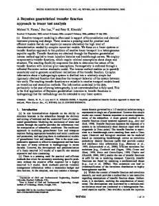
where Q(h)[L 3 /T ] is the flow measured at h, that is the cumulative influx in the interval between the bottom of the borehole (at elevation z o [L]) and the elevation of the EBF (z o + h[L]), and q(ζ )[L 2 /T ] is the flow per unit depth at ζ . All elevations are measured from the same datum. The pumping setup is depicted schematically in Figure 1, where b refers to aquifer saturated thickness. For Dupuit–Forchheimer flow, Darcy’s law can be expressed in radial coordinates as: q(ζ ) = −K (ζ )2πr

dφ dr

(2)

where K (ζ ) is the hydraulic conductivity at ζ , φ is the head, and r is the radial distance from the well. Evaluating Equation (2) at the well: ¯ dφ ¯ q(ζ ) = −2πrw ¯¯ (3) K (ζ ) dr r =rw where rw is the well radius. ) is constant over the depth, the ratio in Equation (3) Assuming the gradient ( dφ dr will be the same for any ζ . Considering the entire thickness of the aquifer, b : q(ζ ) Q(b) = T K (ζ )

(4)

where Q(b) is the total flowrate from the well and T is the aquifer transmissivity.


pp1107-matg-478594

February 10, 2004

15:32



105

Figure 1. Schematic drawing of EBF and pumping setup {not to scale}.

We rearrange to express flowrate per unit depth (unknown) as a function of known (measured) quantities: q(ζ ) =

Q(b) K (ζ ) T

(5)

Substituting Equation (5) into Equation (1), we establish a linear relationship between the quantity we measure (Q(h)) and the unknown quantity we seek (K (ζ )): Z Q(b) zo +h K (ζ ) dζ (6) Q(h) = T zo In this equation, the only unknown is K (ζ ): Q(h) is measured in the EBF, Q(b) is the total flow measured at the pump, and T is known from a constant-rate pump test conducted in one of the boreholes (FW24) and analyzed using Jacob’s straight-line method. Using this formulation, there is not a unique solution for the unknown K (ζ ); the same single-flow measurement could result from one relatively high value of conductivity over a small area, or a small value of conductivity over a larger area. An


pp1107-matg-478594

February 10, 2004

106

15:32



infinite combination of configurations of K (ζ ) could therefore be consistent with observations Q(h 1 ) · · · Q(h n ). A Bayesian approach that considers uncertainty in measurements and in the modeling of spatial variability is therefore well suited to this problem. Initial Setup We can express our forward model in the standard form: y = Hs + v

(7)

where y is an n × 1 vector of measurements (the Q(h) values at discrete measurement depths in this case), H is an n × m algebraic formulation of the forward model function of Equation (6), s is an m × 1 random vector of unknowns, and v is the measurement and model error, modeled as a Gaussian random vector with zero mean and covariance matrix R, in this case: R = vIn where In is an identity matrix of dimension n, and v is the variance. For this work, H is formulated as ( Q(b) 1ζ : ζ j ≥ z i T Hi j = 0 : otherwise

(8)

(9)

where 1ζ is the discretization increment for the m × 1 vector of depths at which the unknown function s is to be estimated, ζ j is the depth of the jth element of s, and z i is the depth of the ith element of the y. In other words, the H matrix serves to implement the integration relating s to y through Riemann sums in a single matrix multiplication. A linear relationship such as Equation (7) allows for the closed-form analytical solutions presented herein to be implemented. As will be shown in the discussion of nonnegativity constraints, some nonlinear problems can be solved using the linear solution form through successive linearizations. In the case of more strongly nonlinear relationships, other methods must be implemented beyond the scope of this work. The variability of s is expressed geostatistically through a Gaussian probability distribution function ( pd f ) constructed using the first two moments: the mean, or prior expected value, and the covariance. The mean of s is: E[s] = Xβ

(10)

where X is a known m × p matrix corresponding to the discretization of the domain in which estimates are to be made, and β are p drift coefficients. In this work,


pp1107-matg-478594

February 10, 2004

15:32



107

p was equal to 2, as discussed below. When p = 2, a zonation approach was employed in which two constant means (β1 and β2 ) apply to two different zones within the domain. The zone locations are defined through the X matrix using the value 1 to indicate a point within a zone, and 0 to indicate a point outside a zone. For example, if the first column in the following matrix indicates zone 1, and the second column zone 2, zone 1 would cover the first two locations, and zone 2 the last three locations (with m = 5 in this example): 

1

 1  X= 0  0 0



0

 0  1   1 1

(11)

Clearly, this approach can be extended for p > 2 to employ more zones. The covariance of s is represented through a generalized covariance function or GCF (Kitanidis, 1997) 1

E[(s − Xβ)(s − Xβ)T ] = Q = κ(η) + C

(12)

where the GCF, κ(η), is a known function of structural parameter η and C is not needed for the solution of the inverse problem. κ(η) was modeled as a linear GCF as described in Kitanidis (1997) κi j = −η|h i − h j | i, j = 1, 2, . . . , m

(13)

where |h i − h j | is the difference in depth of each of the m prediction points from each other within the borehole. Other GCFs could be used, but for this case, the linear GCF was chosen because it is a model imparting a minimum of assumptions about the structure of the function. The linear GCF also yields best estimates with maximum flatness, i.e., that minimize the first derivative of the estimated function (Kitanidis, 1999) thus preventing overshooting of the estimate and resulting in the most direct interpolation between points.

Posterior Probability Density Function The goal of this analysis is to determine the first and second moments of the posterior pdf ( p 00 (s|y)) of the unknown based on the measurements. The posterior


pp1107-matg-478594

February 10, 2004

108

15:32



pdf can be expressed as a function of the prior pdf ( p 0 (s)) and the likelihood function ( p(y|s)) through Bayes’ theorem: p 00 (s | y) = R

p(y | s) p0 (s) p(y | s) p0 (s) ds

(14)

The denominator in Equation (14) is a normalizing constant, and in the linear case, the first two moments of the posterior pdf can be described through the shape (regardless of scaling by a constant) so the equation can be written as: p 00 (s | y) ∝ p(y | s) p0 (s)

(15)

The closed-form solution for Equation (15) is derived in Kitanidis and Vomvoris (1983), Kitanidis (1995), and Snodgrass and Kitanidis (1997) and is summarized in more detail in Appendix A. The equation for ( p 00 (s | y)) is: · ¸ 1 1 p 00 (s | y) ∝ exp − (y − Hs)T R−1 (y − Hs) − (s − Xβ)T Q−1 (s − Xβ) 2 2 (16) where R is the measurement covariance, Q is the prior covariance, and Xβ is the prior mean of s. The posterior pdf is Gaussian so the best estimate is coincident with its peak (or mode). This allows us to disregard the constants and consider only proportionality. Rather than finding the maximum, however, it is easier to find the minimum of the negative logarithm. L ∝ − ln( p 00 (s | y)) L∝

1 1 (y − Hs)T R−1 (y − Hs) + (s − Xβ)T Q−1 (s − Xβ) 2 2

(17) (18)

The drift parameters (β) are also eliminated by working with restricted likelihood (Kitanidis, 1995). The result is: 1 1 (y − Hs)T R−1 (y − Hs) + sT Gs 2 2

(19)

G = Q−1 − Q−1 X(XT Q−1 X)−1 XT Q−1

(20)

L∝ where


pp1107-matg-478594

February 10, 2004

15:32



109

The posterior mean is then found by forming and solving the following cokriging equations "

9 (HX)T

#" # # " HQ HX ΛT = 0p XT M

(21)

where 9 = HQHT + R

(22)

ΛT is an m × n matrix of coefficients, M is a p × n matrix of multipliers, and 0 p is a p × p matrix of zeros. From these results, the posterior mean or best estimate (ˆs) is found as: sˆ = Λy

(23)

V = −XM + Q − QHT ΛT

(24)

with covariance matrix

Confidence intervals are formed using the diagonal elements of V as the variance. For a 95% confidence interval, we form the upper and lower confidence intervals (UCL and LCL) as p UCL = sˆ + 2 diagV p LCL = sˆ − 2 diagV

(25)

Enforcement of Nonnegativity Without constraining the method to yield only positive results, it is possible that conditional realizations of hydraulic conductivity (as manifest in confidence intervals) could extend into negative values. For example, for a mean value near zero applying to a vertical interval, it is entirely possible that large positive values would balance with large negative values, resulting in confidence intervals extending into the negative. The method intrinsically makes no accounting of this and, in many estimation problems, negative values are acceptable. Therefore, nonnegativity must be enforced to reflect the a priori understanding of the physical problem which indicates that negative hydraulic conductivity is not meaningful. Several options for enforcing nonnegativity are available including transforms into logarithmic space (Kitanidis, 1997), normal score transformations (Deutsch


pp1107-matg-478594

February 10, 2004

110

15:32



and Journel, 1992), and Markov Chain Monte Carlo (MCMC) methods with Lagrange multipliers (Michalak and Kitanidis, 2003). The straightforward power transformation (Box and Cox, 1964; Snodgrass and Kitanidis, 1997) was selected: ¡ 1 ¢ s = α kα − 1

(26)

with the back-transformation µ k=

s+α α

¶α

.

(27)

Note that in the limit ¢¢ ¡ ¡ 1 s = lim α k α − 1 = ln(k) α→∞

(28)

and the back-transformation µ k = lim

α→∞

s+α α

¶α

= exp(s)

(29)

For reasonable values of α, any value of s will be back-transformed to a positive value of k. Kitanidis and Shen (1996) provide a method for optimally determining α. However, for this work, a relatively large value of α (102 ) is used to approximate the logarithmic transformation. Using this transformation the measurement equation becomes: µ

s+α y=H α

¶α

+v

(30)

This relationship is not linear, so iterative techniques are necessary for the 1 determination of the best estimate of s = sˆ. For the first iteration, the best estimate sˆ was chosen as the transformed best estimate from the linear case (i.e. the case where nonnegativity was not enforced) using the transformation of Equation (26). In the few instances where a negative best estimate value was encountered, a small positive number was substituted. It is not necessary to first calculate the linear result to use as a seed value, but the value should be close to the final best estimate, and may reduce the number of iterations in the solution. We employ the quasi-linear technique of Kitanidis (1995) using successive linearization. We first must linearize the problem in a Taylor series resulting in yl = Hl s + v

(31)


pp1107-matg-478594

February 10, 2004

15:32



111

where (yl )i = yi −

µ

m X

Hi j

j=1

sˆ j + α α

¶α ·

αˆs j 1− sˆ j + α

¸ (32)

and µ (Hl )i j = Hi j

sˆ j + α α

¶α µ

¶ α . sˆ j + α

(33)

In these equations, sˆ is the best estimate of s about which the Taylor expansion is performed. Details of the Taylor expansion are provided in Appendix B. The linear techniques described above are then applied to this linearized equation iteratively, until the solution converges. From the solution we obtain the best estimate and confidence intervals.

Structural Parameter Optimization Thus far, the two structural parameters in this problem " #! v θ= η

Ã

1

have been assumed known. These parameters describe variability in the model, measurements, and estimation and derive from Equations (8) and (13). In practice, they must be found by optimization by maximizing the probability of the measurements given the parameters: · ¸ 1 1 1 p(y | θ) ∝ (det Ψ)− 2 (det[XT HT 9 −1 HX])− 2 exp − yT Ξy 2

(34)

where Ψ = HQHT + R 4=9

−1

−9

−1

(35)

HX(X H 9 T

T

−1

HX)X H 9 T

T

−1

(36)

It is easier to minimize the logarithm of p(y | θ) as L(θ) =

1 1 1 ln(det Ψ) + ln(det[XHΨHX]) + yT Ξy 2 2 2

(37)


pp1107-matg-478594

February 10, 2004

112

15:32



The minimization is performed by setting the derivatives of Equation (37) equal to zero, and finding the values of θ that satisfy the equation using the Gauss– Newton method. The Gauss–Newton method is performed as described in Kitanidis (1995).

Algorithm Summary Following is a brief summary of the algorithm. 1. Determine an initial estimate of the unknown (ˆs0 ). 2. Select a value for α to be used in the power transformation. If in doubt, use a high value of α to approximate a natural logarithmic transformation. 3. Transform both sˆ0 and the measurements (y) using the power transformation. 4. Determine an initial guess for the structural parameters Ã

" θ=

v0

#!

η0

5. Linearize the problem, obtain a new best estimate by solving the system in Equations (21) and (23) for the Λ, and calculating µ sˆ =

Λyl + α α

¶α

.

6. Set sˆ0 = sˆ, and iterate until the change in sˆ from one iteration to the next is sufficiently small. 7. Using the values yl and Hl , calculate optimal structural parameters as in the linear case. 8. Once the structural parameter optimization has converged, calculate a final best estimate and set of confidence intervals using the optimal parameters and repeat steps 5–7. 9. Back-transform the results to physical space using Equation (27).

First-Difference Method The traditional method for deterministic interpretation of borehole flowmeter tests is the first-difference method, as discussed in the introduction. In this method the flux between two adjoint measurement points is evaluated from the difference between the measured fluxes; then, the average or effective conductivity is


pp1107-matg-478594

February 10, 2004

15:32



113

estimated for the interval K (ζ ) =

Q(h i+1 ) − Q(h i ) T , h i < ζ < h i+1 h i+1 − h i Q(b)

(38)

The value obtained applies to the entire interval (h i to h i+1 ), and for plotting and subsequent calculations, the value was used as a point-value at the center of the vertical section ( h i +h2 i+1 ). Ordinary Kriging Ordinary kriging was performed on the results of the first-difference method to provide an alternative and easier way to account for uncertainty in the estimates of hydraulic conductivity. Variogram fitting and Kriging calculations were implemented following the cR and Q2 optimization methodology in Kitanidis (1997) using code from Erickson (1999). First-difference data were transformed using the power transform in Equation (26). A nugget effect was introduced to accompany the linear variogram in order to suppress small-scale variations in the solution. Although a different variogram may be more appropriate, the linear variogram with nugget was chosen to foster meaningful comparison with the Bayesian results. It was neither possible to perform indicator kriging nor zonation for kriging due to the limited data points in the lower zone in FW24.

DATA AND RESULTS The techniques discussed above were applied to flowmeter test results from the Field Research Center (FRC) at the Oak Ridge Reservation (ORR). First is a discussion of the data obtained, preliminary processing and evaluation of the data, and an explanation of which data were ultimately used for this analysis. Following the discussion of data is the presentation and interpretation of the results from the FRC, and a comparison of results from the three methods. Data The electromagnetic borehole flowmeter (EBF) tests used in this study were performed at the FRC in April and May of 2001 (Waldrop and Pearson, 2001). Two boreholes were tested and are labeled FW24 and FW26. The two boreholes are approximately 3.4 m apart (Fig. 2). Data pertaining to flow measured in the field, and vertically averaged hydraulic conductivity are both needed to determine the vertical distribution of hydraulic conductivity. The vertically averaged hydraulic


114

pp1107-matg-478594

February 10, 2004

15:32



Figure 2. Location of the boreholes FW24 and FW26.

conductivity was independently determined from a constant-rate pumping test in borehole FW24. Ambient or regional flow must be removed because natural vertical gradients may work with or against the pumping and could over- or underestimate the stress induced on the aquifer by pumping (Young and others, 1998). Ambient flow was measured prior to perturbation of the well. The EBF was placed at various intervals starting at the bottom of the borehole, and a packer was inflated isolating the EBF so flow measured at each interval was the total cumulative flow between the bottom of the borehole and the EBF. For this test, positive EBF measurements indicate upward ambient flow, while negative measurements indicate downward ambient flow. Pumping induced flow was also positive, so the following correction for ambient flow was made: Q(h)net = Q(h)pumped − Q(h)ambient

(39)

where the dependence on (h) indicates that flow is measured at various depths. After determining the ambient flowrate, the velocity was measured again using the EBF in the same manner while pumping. First each borehole was pumped at a rate of approximately 1.5 L per min (LPM) until drawdown reached steady


pp1107-matg-478594

February 10, 2004

15:32



115

state. The pump was then placed near the water table and a constant pump rate was maintained. By maintaining a constant total pump rate, variations in flow measured through the EBF as a function of depth are known to result from variations in the hydraulic conductivity of the formation. Several difficulties were encountered in the execution of the field tests resulting in underestimation of flow readings toward the end of the test. These difficulties resulted in limitations to the usability of the data, and some preliminary data selection was necessary as discussed below. Borehole FW24 Flowmeter Data Borehole FW24 was the more successful of the two tests. However, the field crew encountered difficulty in obtaining a proper seal with the packer in loose soil near the top of the borehole. Therefore, some flow likely bypassed the EBF resulting in underestimated flow readings. This hypothesis was qualitatively tested by briefly overinflating the packer and attempting to read the flow on the EBF. The flowrate at the instant of overinflation was observed to be in line with that expected, but a stable reading (the average of several sequential readings) was not possible. Therefore, several data points were disregarded near the top of the column. The shallowest point (near the water table) was replaced by the total flow measured from the well because all flow must have exited the borehole through the shallowest point. The EBF readings are presented in Figure 3 where open squares show all readings recorded, open diamonds show ambient flow, and filled triangles show net corrected flow at the elevations where measurements were retained. Borehole FW26 Flowmeter Data The lithologic similarity and close proximity of borehole FW26 to FW24 suggest that some difficulty obtaining a good seal with the packer in the upper section of the borehole may have been encountered in FW26. However, this concern was eclipsed by more serious problems caused by variations in the pump rate. The pumping rate varied dramatically when the flowmeter was at shallow depth, masking the flowrate signal resulting from variations in lithology. Therefore, at depths shallower than about 11 m, the flow values are not considered reliable (Fig. 4). Fortunately, these shallow points are expected to contribute little to the overall flow, and hence the region of rejected data is interpreted to be of low hydraulic conductivity. Similarly to FW24, the shallowest data point was assigned a value equal to the total pump flowrate. All data points between the shallowest depth and 11 m were not used, with the exception of the data point at 9.14 m (30 ft). This data point was interpreted to be in line with the expected flow rate and was retained in


116

pp1107-matg-478594

February 10, 2004

15:32



Figure 3. Vertical flow profile for FW24.

Figure 4. Vertical flow profile for FW26.


pp1107-matg-478594

February 10, 2004

15:32



117

the analysis. Finally, the deepest point was set to zero due to field observations that there was no flow at this depth (Waldrop and Pearson, 2001). The EBF readings are presented in Figure 4 following the same convention as for FW24 above. RESULTS The results of the three methods are first discussed separately, and then compared. Bayesian Inverse Method The flow profiles (Figs. 3 and 4) were analyzed assuming a single constant mean (i.e. a single zone) throughout the entire depth of the formation. The structural parameters did not converge for FW24, but they did for FW26, resulting in a hydraulic conductivity profile (Fig. 5). The inability of structural parameters to converge in the case of FW24 is a result of the extreme variability in the initial flow profile. In FW24, two regions or zones of flow behavior can be discerned (Fig. 3). A significant increase in flow per unit depth is observed at the bottom of the borehole, indicating high hydraulic conductivity. However, at approximately 10.9 m bls, an abrupt change is seen, and the flow increases with decreasing depth at a much lower rate, indicating lower hydraulic conductivity. It is unreasonable

Figure 5. Hydraulic conductivity in FW26 (Bayesian inverse method): No zonation.


118

pp1107-matg-478594

February 10, 2004

15:32



to expect a linear model of variance to capture two distinct, smoothly varying patterns. Favoring parsimony, the GCF was retained and a zoned approach was followed. This allows the same number of structural parameters to be optimized while also allowing for two mean values (β). We know a priori that the aquifer has fractured zones, and we also expect a weathering contact to be encountered. Such an obvious jump in flow indicates that a distinct difference in lithology is apparent, further suggesting use of a zoned model. The zone boundary was chosen as the depth at which the obvious inflection point in the flow curve was observed. Both data sets were reexamined using the zoned approach because similar geologic conditions are present at both borehole locations. With the zoned approach, the structural parameters for FW24 converged rapidly to reasonable values (Fig. 6). The behavior and results of FW26 were also reasonable when subjected to the zoned approach (Fig. 7). In this borehole, the zone transition was assigned as 11.9 m bls. In general, the results of the best estimate match the pattern expected based on the geology of the site. An increase in hydraulic conductivity with depth was expected within the transition zone before more competent rock was encountered at the bottom of the borehole. The convergence of the structural parameter

Figure 6. Hydraulic conductivity in FW24 (Bayesian inverse method): Range is trimmed at upper end, affecting only three UCL measurements which had a maximum value of 0.0126 cm/s. Zoned approach with zone transition is at 10.9 m bls.


pp1107-matg-478594

February 10, 2004

15:32



119

Figure 7. Hydraulic conductivity in FW26 (Bayesian inverse method): Zoned approach with zone transition set at 11.9 m bls.

optimization (especially in FW24) was very sensitive to the location of the zone boundary. First-Difference and Ordinary Kriging Methods Both the first-difference and ordinary kriging results were computed (Figs. 8 and 9). These results are presented together because the first-difference results were the data used as the basis for the ordinary kriging. Comparison of Results Figures 10 and 11 present the comparison of the first-difference, ordinary kriging, and inverse methods for deconvoluting the hydraulic conductivity profile. Only the best estimates are presented. The general patterns of the best estimates among the three methods are similar. The first-difference method provides one result for each measurement taken which applies to the entire interval sampled in a given event. No uncertainty analysis is possible with the first-difference method. Both the Bayesian inverse method and ordinary kriging provide estimates of the function at intermediate points on an arbitrary discretization. Furthermore, both methods offer formal estimation of uncertainty. Kriging, however, does not allow for a physically relevant forward model to be explicitly incorporated. In a


120

pp1107-matg-478594

February 10, 2004

15:32



Figure 8. Hydraulic conductivity in FW24 (first-difference and ordinary kriging): Range is trimmed at upper end, affecting only two UCL measurements which had a maximum value of 0.0201 cm/s.

Figure 9. Hydraulic conductivity in FW26 (first-difference and ordinary kriging).


pp1107-matg-478594

February 10, 2004

15:32



Figure 10. Hydraulic conductivity in FW24: Comparison of three deconvolution methods.

Figure 11. Hydraulic conductivity in FW26: Comparison of three deconvolution methods.

121


122

pp1107-matg-478594

February 10, 2004

15:32



case as this problem where a simplified forward model is used, the difference in results is not substantial. However, with a more complicated forward model, the explicit incorporation of such a model may result in a superior solution using the Bayesian inverse method rather than kriging. CONCLUSIONS We have developed a Bayesian inverse method for the deconvolution of hydraulic conductivity in borehole flowmeter tests. A linear GCF was an appropriate model of the prior covariance when combined with the zonation approach. Without zonation, it was not possible to obtain results for one borehole (FW24) and results in both boreholes tested were improved through use of the zonation model. The quasi-linear Bayesian inverse method applied here assumes a Gaussian prior distribution, which encounters difficulty at geologic contacts or other discontinuities. A different prior distribution may be better suited to handle such discontinuities without the need for zonation. However, the zonation approach has the advantage of being intuitive with respect to the geology at the site. Ordinary kriging with a linear variogram and nugget effect was also performed for comparison, and the results of the inverse method and kriging were both compared to results of the traditional first-difference method. Both the Bayesian inverse method and kriging take into account errors and variability and provide a best estimate and confidence intervals. Both methods also yielded reasonable results as compared to the traditional first-difference method, and all results of all three methods were consistent with the geology at the site. It was expected that higher hydraulic conductivity would be encountered at depth due to a transition from highly weathered saprolite to fresher fractured shale with increasing depth. The enforcement of nonnegativity through use of a power transformation was critical in obtaining physically reasonable estimates of hydraulic conductivity. For the Bayesian inverse method, successive linearization and optimization using the Gauss–Newton method was effective both in handling the nonlinearity resulting from the power transformation, and in obtaining optimal structural parameters. This method of enforcing nonnegativity suffers from the fact that confidence intervals are dependent on the magnitude of measurements which may not be appropriate with varied magnitudes of best estimates. The ordinary kriging approach has the advantage of being relatively easy to implement using a variety of commercially available programs. This approach is directly dependent on the first-difference results, however, overemphasizing the importance of the midpoints of sampled intervals. The Bayesian inverse method is more involved to implement but, when combined with zonation, provides reasonable and usable results. The Bayesian method also explicitly incorporates the physics of the problem in the forward model. In the instance of the simplified forward model of this case, this advantage was not


pp1107-matg-478594

February 10, 2004


15:32


123

strong, but with a more realistic forward model, the closer honoring of the physics could grow in significance. Preliminary data screening also added to the physical reasonability of the results, as several EBF measurements were rejected as a result of field observations. ACKNOWLEDGMENTS This work was partially funded by the National Defense Science and Engineering Graduate fellowship program, and the United States Department of Energy (DOE), Natural and Accelerated Bioremediation Research (NABIR), Biological and Environmental Research (BER) grant number (#DE-F603-00ER63046). The authors also thank Professor Craig Criddle for ongoing insights, the Oak Ridge National Laboratory Field Research Center for providing the data, and DOE technical representatives Anna Palmisano and Paul Bayer for their financial support. Anna Michalak provided valuable comments which improved the manuscript. REFERENCES Bailey, Z. C., 1988, Preliminary evaluation of ground-water flow in Bear Creek Valley, The Oak Ridge Reservation, Nashville, TN: U.S. Geological Survey Report: WRI 88-4010, 12 p. Box, G. E. P., and Cox, D. R., 1964, An analysis of transformations: J. R. Stat. Soc. B (Methodol.) v. 26, no. 2, p. 211–252. Christakos, G., 1990, A Bayesian/maximum-entropy view to the spatial estimation problem: Math. Geol., v. 22, no. 7, p. 763–777. Deutsch, C. V., and Journel, A. G., 1992, GSLIB: Geostatistical software library and user’s guide: Oxford University Press, New York, 369 p. Dorsch, J., Katsube, T. J., Sanford, W. E., Dugan, B. E., and Tourkow, L. M., 1996, Effective porosity and pore throat sizes of Conasauga Group Mudrock: Application, test and evaluation of petrophysical techniques: U.S. Department of Energy, Report ORNL/GWPO-021, Oak Ridge National Laboratory, Oak Ridge, TN. Erickson, T. A., 1999, Contributions to best linear unbiased estimation: Unpublished Thesis, Stanford University, Department of Civil and Environmental Engineering, 78 p. Jacobs EM Team, 1997, Feasibility study for Bear Creek Valley at the Oak Ridge Y-12 Plant, Oak Ridge, TN: Volume II: Appendixes [sic]: U.S. Department of Energy, Office of Environmental Management, Oak Ridge, p. F-1–F-109. Jardine, P. M., Wilson, G. V., Luxmoore, R. J., and Gwo, J. P., 2001, Conceptual model of vadose-zone transport in fractured weathered shales. Conceptual models of flow and transport in the fractured vadose zone: National Academy Press, Washington, p. 87–114. Kitanidis, P. K., 1995, Quasi-linear geostatistical theory for inversing: Water Resour. Res. v. 31, no. 10, p. 2411–2419. Kitanidis, P. K., 1997, Introduction to geostatistics: Applications in hydrogeology: Cambridge University Press New York, 249 p. Kitanidis, P. K., 1999, Generalized covariance functions associated with the Laplace equation and their use in interpolation and inverse problems: Water Resour. Res. v. 35, no. 5, p. 1361–1367.


pp1107-matg-478594

February 10, 2004

124

15:32



Kitanidis, P. K., and Shen, K. F., 1996, Geostatistical interpolation of chemical concentration: Adv. Water Resour. v. 19, no. 6, p. 369–378. Kitanidis, P. K., and Vomvoris, E. G., 1983, A geostatistical approach to the inverse problem in groundwater modeling (steady state) and one-dimensional simulations: Water Resour. Res. v. 19, no. 3, p. 677–690. Lozier, W. B., Spiers, C. A., and Pearson, R., 1987, Aquifer pump test with tracers: Golder Associates, Atlanta, GA, 98 p. Michalak, A. M., and Kitanidis, P. K., 2003, A method for the enforcing parameter nonnegativity in Bayesian inverse problems with an application to contaminant source identification: Water Resour. Res. v. 39, no. 2, p. 1033–1047. Molz, F. J., Boman, G. K., Young, S. C., and Waldrop, W. R., 1994, Borehole flowmeters; field application and data analysis: J. Hydrol. v. 163, no. (34), p. 347–371. Snodgrass, M. F., and Kitanidis, P. K., 1997, A geostatistical approach to contaminant source identification: Water Resour. Res. v. 33, no. 4, p. 537–546. Solomon, D. K., Moore, G. K., Toran, L. E., Dreier, R. B., and McMaster, W. M., 1992, A hydrologic framework for the Oak Ridge Reservation, Oak Ridge, TN: U.S. Department of Energy, Oak Ridge National Laboratory, Environmental Sciences Division, 70 p. Waldrop, W. R., and Pearson, H. S., 2001, Results of field test with the electromagnetic borehole flowmeter at the Oak Ridge National Laboratory, Oak Ridge, TN: Quantum Engineering Corporation, Loudon, TN, 17 p. Woodbury, A. D., and Ulrych, T. J., 1998, Minimum relative entropy and probabilistic inversion in groundwater hydrology: Stochastic Hydrol. Hydraulics v. 12, no. 5, p. 317–358. Young, S. C., Julian, H. E., Pearson, H. S., Molz, F. J., and Boman, G. K., 1998, Application of the electromagnetic borehole flowmeter: United States Environmental Protection Agency, Cincinnati, OH, 71 p.

APPENDIX A: DERIVATION OF POSTERIOR PDF The Gaussian prior pdf, p 0 (s), can be readily constructed from the expected value and covariance matrix. µ ¶ 1 1 0 T −1 exp − (s − Xβ) Q (s − Xβ) (A1) p (s) = √ 2 det Q The likelihood function (Kitanidis, 1995) can be expressed as µ ¶ 1 1 exp − (y − h(s, r))T R−1 (y − h(s, r)) p(y | s) = √ 2 det R

(A2)

Equation (6) is linear, so we can express the integral and the constant parameters (r) as Riemann sums, and express Equation (7) as y = Hs + v

(A3)

where H is a known matrix representing the function of Equation (6). The constant parameters Ã " #! Q(b) r= T (b)


pp1107-matg-478594

February 10, 2004

15:32



125

are absorbed into H. The expected value of the measurements given the unknowns is found through the discretized forward Equation (A3). The covariance is R, as defined above. Therefore, the likelihood function is expressed as p(y | s) = √

µ

1 det R

exp

¶

1 − (y − Hs)T R−1 (y − Hs) 2

(A4)

Multiplying these pdfs results in the posterior pdf: · ¸ 1 1 p 00 (s | y) ∝ exp − (y − Hs)T R−1 (y − Hs) − (s − Xβ)T Q−1 (s − Xβ) 2 2 (A5)

APPENDIX B: LINEARIZATION OF THE MEASUREMENT EQUATION We introduce a power transformation of the hydraulic conductivity vector k ¡ 1 ¢ s j = α k jα − 1 ,

s j > −α

(A6)

so the observation equation becomes yi =

m X

µ Hi j

j=1

sj + α α

¶α

+ vi ,

i = 1, . . . , n.

(A7)

Equation (A7) is nonlinear, so we expand in a Taylor series about an estimate of s which we call sˆ. The expansion of the nonlinear term is: µ

sj + α α

¶α

µ =

sˆ j + α α

¶α

µ +

sˆ j + α α

¶α µ

α sˆ j + α

¶µ

¶ s j − sˆ j

+ H.O.T. (A8)

where H.O.T. means higher (than linear) order terms. Neglecting the higher-order terms, Equation (A7) becomes, after rearrangement of terms, yi − µ ×

m X j=1

µ Hi j

sˆ j + α α

¶ α s j + vi , sˆ j + α

¶α ·

¸ X ¶ µ m sˆ j + α α αˆs j Hi j = 1− sˆ j + α α j=1

i = 1, . . . , n

(A9)


pp1107-matg-478594

February 10, 2004

126

15:32



Thus, we obtain the linearized system, (yl )i =

m X (Hl )i j s j + vi ,

i = 1, . . . , n

(A10)

j=1

where (yl )i = yi −

m X

µ Hi j

j=1

µ (Hl )i j = Hi j

sˆ j + α α

sˆ j + α α ¶α µ

¶α ·

α sˆ j + α

1−

αˆs j sˆ j + α

¸ (A11)

¶ (A12)

An Application of Bayesian Inverse Methods to ... - Stanford University

An Application of Bayesian Inverse Methods to ... - Stanford University

Suggest Documents

Application of Bayesian Methods to Exposure

An application of Bayesian statistical methods to adaptive ... - Deep Blue

Application of an inverse solution to the ... - University of Utah

Subgradient Methods - Stanford University

Frequentist Accuracy of Bayesian Estimates - Stanford University

Grasping with Application to an Autonomous ... - Stanford University

Envelope condition method with an application to ... - Stanford University

Envelope condition method with an application to ... - Stanford University

Application of Bayesian Methods to Habitat Selection Modeling of the ...

Application of Bayesian Methods to Habitat Selection Modeling of the ...

A Bayesian geostatistical transfer function ... - Stanford University

An Application of Hierarchical Bayesian Modelling - University of Otago

Learning Causal Bayesian Network Structures ... - Stanford University

Learning Causal Bayesian Network Structures ... - Stanford University

Bayesian Ascent - Engineering Informatics Group - Stanford University

Bayesian Inverse Reinforcement Learning

Hierarchical Bayesian Approaches to the Inverse

Application of incremental Gaussian mixture ... - Stanford University

Application of Ion Chromatography to the ... - Stanford University

application of surface impedance approach to ... - Stanford University

Generalized hybrid iterative methods for large-scale Bayesian inverse ...

The application of neuroimaging to social ... - Stanford University

The application of neuroimaging to social ... - Stanford University

application of x-ray tomography to measurement ... - Stanford University