144
JOURNAL OF APPLIED METEOROLOGY
VOLUME 44
An Application of the Variational Method to Computation of Sensible Heat Flux over a Deciduous Forest ZUOHAO CAO
AND
JIANMIN MA
Meteorological Service of Canada, Burlington, Ontario, Canada (Manuscript received 3 December 2003, in final form 18 June 2004) ABSTRACT A variational method is employed to compute surface sensible heat fluxes over a deciduous forest using observed temperature, temperature variance, and wind. Because the variational approach is able to take into account comprehensive observational meteorological conditions over a heterogeneous surface, it is applicable to the computations of sensible heat flux over a forest canopy in which the conventional fluxvariance method is difficult to use. Verifications using the direct eddy-correlation measurements over a deciduous forest during the fully leafed summer of 1988 and the leafless winter of 1990 show that the variational method yields very good agreements between the computed and the measured sensible heat fluxes. It is also shown that the variational method is much more accurate than the flux-variance method in computations of sensible heat flux over a forest canopy.
1. Introduction Surface sensible heat flux is an important quantity to measure energy exchange between the surface and the atmosphere. Many attempts have been made to accurately compute the sensible heat flux over relatively flat and open surfaces. Because of the homogeneous nature of these surfaces, the flux-gradient relations, derived from the Monin–Obukhov similarity theory (MOST) applicable for an equilibrium flow/small eddy activity over a flat homogeneous surface, are applied to estimate the sensible heat flux. However, within and immediately above a forest canopy, the transfer mechanisms for sensible heat are substantially different from those over an open field. Departures of sensible heat fluxes from the flux-gradient relations over a forest have been reported for about 3 decades (e.g., Thom 1975; Raupach 1979). Efforts have been made toward establishing physically sound theories of turbulence and atmospheric transfer processes in forest canopies (e.g., Garratt 1994). Mölder et al. (1999) applied the roughness sublayer corrections with enhanced eddy diffusivities to flux-gradient relationships over a boreal forest. Although some improvements were made with the modified flux-gradient relationship, the corrected fluxes were still scatter compared with observations (Mölder et al. 1999). Field observations (Gao et al.
Corresponding author address: Dr. Zuohao Cao, Meteorological Service of Canada, 867 Lakeshore Road, P. O. Box 5050, Burlington, ON L7R 4A6, Canada. E-mail:
[email protected]
© 2005 American Meteorological Society
JAM2179
1989) and wind tunnel experiments (Raupach et al. 1986) have revealed that large eddy organized turbulent motions dominate the transport of momentum, heat, and moisture within and above forest canopies. In addition, the MOST-based flux-variance relations were developed for computations of sensible heat fluxes (Wyngaard et al. 1971; Wesely 1988; Weaver 1990; Lloyd et al. 1991; de Bruin et al. 1991, 1993; Padro 1993; Katul et al. 1995; Katul and Hsieh 1999). Although some agreements between the measured and the estimated sensible heat fluxes are obtained using the flux-variance relations for bare soil, fallow savannah, and tiger bush surfaces (Lloyd et al. 1991), the variance techniques do not always produce reliable estimates of fluxes of scalar quantities (Wesely 1988), particularly if the surface is nonuniform where the heat advection may occur or a flux is small in magnitude (Weaver 1990; Wesely 1988; Katul et al. 1995). As an alternative, the variational method appears promising in computing sensible heat flux (Xu and Qiu 1997; Xu et al. 1999; Zhou and Xu 1999). The variational method, in principle, minimizes the differences between the calculated and the measured quantities of meteorological variables so that it can adjust the calculated flux toward the observed one. By doing this, one can make full use of the observed meteorological information over a heterogeneous surface. In other words, the influences of actual meteorological conditions and surface heterogeneities on the computations of surface fluxes can be automatically taken into account in the procedures of implementing the variational method. To date, most (if not all) successful computations of
JANUARY 2005
sensible heat flux using the variational method are performed over a flat homogeneous surface (Xu and Qiu 1997; Xu et al. 1999; Zhou and Xu 1999). Little work has been done using the variational approach to compute sensible heat flux over a heterogeneous surface. In this study, we intend to extend the variational method to the computation of sensible heat fluxes over a forest canopy and to obtain reliable estimations of the sensible heat flux based on measurements of temperature, temperature variance, and wind. Furthermore, we attempt to verify the variational-method-computed sensible heat flux against direct eddy-correlation measurements and to compare with those computed by the conventional flux-variance method. Section 2 briefly reviews two conventional methods and the variational method for computations of sensible heat flux. After describing the datasets used for computation of sensible heat flux in section 3, we present the computational results of sensible heat fluxes and compare the calculated fluxes with the eddycorrelation measured fluxes in section 4. The conclusions are then given in section 5.
2. Methodology a. Flux-gradient relation The flux-gradient relation used for computation of heat flux Fh can be described in the following two coupled equations (e.g., Yaglom 1977): u⫽
冋冉
冊 冉 冊 冉 冊册
u* z2 ⫺ d z2 z0m ln ⫺ m ⫹ m z0m L L
T2 ⫽ T1 ⫺
冋冉
and
冉冊
冉 冊 冉 冊
z2 1 ⫹ x2 1 ⫹ x22 ⫽ 2 ln ⫹ ln L 2 2 ⫺ 2 tan⫺1共x2兲 ⫹
2
h
冉冊
冉
z2 1 ⫹ y2 ⫽ 2 ln L 2
冊
for unstable conditions (z/L ⬍ 0), where
冉
x2 ⫽ 1 ⫺ ␥m
z2 L
冊
1Ⲑ4
冋
and y2 ⫽ 1 ⫺ ␥h
冉 冊册 z2 L
1Ⲑ2
,
and
m
冉冊
冉冊
z2 z2 ⫽ ⫺m L L
and h
冉冊
冉冊
z2 z2 ⫽ ⫺h L L
for stable conditions (z/L ⬎ 0). The constants ␥m, ␥h, m, and h are equal to 15, 9, 4.7, and 6.35, respectively (Businger et al. 1971). Since the Borden data used in this study are only available at z2 (⫽33.4 m), there are essentially three unknowns in Eqs. (1) and (2): the friction velocity u*, the heat flux Fh, and the temperature T1. If these three unknowns need to be determined from these two equations, the mathematical problem is intrinsically underdetermined. Under this circumstance, the flux-gradient relation itself cannot be properly applied to computation of sensible heat flux. However, Eqs. (1) and (2) can be used in the flux-variance-based and variationalmethod-based computations, as described in the next sections. It should be mentioned that the zero-plane displacement height d ⫽ 13 m (e.g., Lo 1995) is used in this study. The results show that the variationalmethod-computed sensible heat fluxes are not sensitive to the zero-plane displacement.
b. Flux-variance relation
共2兲
There exist several types of the flux-variance equations for computation of heat flux (e.g., Wesely 1988; Tillman 1972). In this study, we use the approach that employs a normalized variance to compute the heat flux:
冊 冉 冊 冉 冊册
Fh z2 ⫺ d z2 z1 ln ⫺ h ⫹ h u* z1 ⫺ d L L
and
共1兲 ,
where , L, u*, z0m, and d are, respectively, the von Kármán constant (⫽0.4), the Monin–Obukhov length, the friction velocity, the aerodynamic roughness length [z0m ⫽ 1 m for a forest canopy (see Lo 1995; Padro et al. 1991)], and the zero-plane displacement (Lo 1995). In Eq. (2), Fh ⫽ (w⬘T⬘)0 (⫽⫺u*T*, where T* is the flux temperature scale) is the heat flux; T1 and T2 are the air temperature at two vertical levels z1 (⫽18 m) and z2 (⫽33.4 m); and m and h in Eqs. (1) and (2) are integral forms of the departure of the wind speed and the temperature from their neutral values, defined at z2 as
m
145
CAO AND MA
| Fh | ⫽ T
u*
共zⲐL兲
共3兲
,
where T is a temperature variance, and is a dimensionless universal function of stability z/L (Panofsky and Dutton 1984). Based on Panofsky and Dutton (1984), Hicks (1981), Padro et al. (1992), Wesely (1988), and Weaver (1990),
共zⲐL兲 ⫽ a1 ⫺1Ⲑ3
⫽ a2共⫺zⲐL兲
for
zⲐL ⬎ 0
for
zⲐL ⬍ 0,
共4兲
where a1 and a2 are 1.85 and 1.0, respectively (Wyngaard et al. 1971; Panofsky and Dutton 1984). Following Weaver (1990), we use the first equation in Eq. (4) for stable and near-neutral conditions, and the second equation in Eq. (4) for unstable conditions. According
146
JOURNAL OF APPLIED METEOROLOGY
to Katul et al. (1995), the Monin–Obukhov length can be computed as follows: L⫽⫺
g
冉
u3* H ⫹ 0.61E cpT2
冊
,
共5a兲
where is the air density, cp is the specific heat of air at constant pressure, g is the gravitational acceleration, H is the sensible heat flux, and E is the evaporation rate. If the experiment site is assumed to be dry, the Monin– Obukhov length can be simplified as u3T2 L⫽⫺ * . gFh
共5b兲
In Eqs. (1) and (3), two unknown variables, u* and Fh, can be solved by an iterative procedure (e.g., de Bruin et al. 1993).
c. Variational method The MOST-based flux-gradient and flux-variance methods are, in principle, applicable for small eddy activities in the atmospheric boundary layer over a homogeneous terrain, but the variational method can allow us to fully utilize actual observed meteorological conditions over a heterogeneous surface through a procedure to minimize the difference between observed and computed meteorological variables. This difference is defined herein as a cost function J to measure errors between the computed and observed temperature, temperature variance, and wind speed (e.g., Xu and Qiu 1997; Xu et al. 1999; Zhou and Xu 1999; Ma and Daggupaty 2000): 1 obs 2 2 J ⫽ 关WT 共T2 ⫺ T obs 2 兲 ⫹ W共T ⫺ T 兲 2 ⫹ Wu共u ⫺ uobs兲2兴.
共6兲
The cost function J defined by the differences in Eq. (6) is actually considered as the function of (u*, Fh, T1) in obs obs the variational method. In Eq. (6), T obs 2 , T , and u are the observed temperature at z2 (⫽33.4 m), the temperature variance, and the wind speed at z2 (⫽33.4 m), respectively; WT, W, and Wu are weights for the temperature, the temperature variance, and the wind speed. The weights are, in general, chosen to be inversely proportional to their respective maximally tolerated observation error variances (Xu and Qiu 1997) so that J is minimized to give the optimal estimates of the temperature, the temperature variance, and the wind speed. The weights are usually difficult to determine precisely because of uncertainties in measurement errors. In reality, the weights can be specified empirically and even arbitrarily (Daley 1996). In this study, the estimated values of weights are used as follows: WT ⫽ 0.8 (K⫺2), W ⫽ 12 (K⫺2) and Wu ⫽ 10 (m⫺2 s2). As shown in section 4, the variational computations are not
VOLUME 44
very sensitive to the choice of the weights. To determine u, T2, and T in the cost function, the flux-gradient relations [Eqs. (1) and (2)] and the flux-variance relation in Eq. (3) are employed. It should be pointed out that the constants a1 and a2 in the universal function Eq. (4) have been found to be quite sensitive to source (or sink) heterogeneity of a scalar (Katul et al. 1995; Andreas et al. 1998). Using the Borden datasets and Weaver’s (1990) method, Padro et al. (1992) obtained different values of a1 ranging from 1.9 to 12.37 and of a2 ranging from 0.65 to 4.23 for different scalar quantities. These values are different from the common values of a1 ⫽ 1.85 and a2 ⫽ 1. Padro et al. (1992) claimed that adjusting the values of a1 and a2 could result in better agreement between estimated fluxes using Eq. (3) and measured fluxes. In this study, a1 ⫽ 2.54 and a2 ⫽ 1 (Padro et al. 1992) are used. The choice of physical constraints in the cost function may vary in terms of targeting parameters and variables to be retrieved (Ma and Daggupaty 2000). In the present study, the minimization of the cost function J is carried out to give optimal estimates of Fh, u*, and T1, which requires that the gradients of J with respect to unknown variables Fh, u*, and T1 become zero: ⭸J ⭸J ⭸J ⫽ ⫽ 0. ⫽ ⭸Fh ⭸u* ⭸T1
共7兲
The analytic formulations of these gradient components are presented in the appendix. A quasi-Newton method is applied to find the minimum of the cost function J. This method requires an iterative procedure to compute the cost function Eq. (6) and its gradients Eq. (7), that is, Eqs. (A1)–(A12), and to determine the minimum of J along a search direction. For Eq. (6), the inputs are the measured u, T2, and T, and the outputs are calculated u, T2, and T and estimated Fh, u*, and T1. The following iterative procedure is used to compute the cost function and its gradient and to derive Fh, u*, and T1: 1) Set up initial guesses of unknowns, say, u* ⫽ 0.4 m s⫺1, Fh ⫽ 0.2 K m s⫺1, and T1 ⫽ 280 K. 2) Calculate and L from Eqs. (4) and (5b). 3) Calculate u, T2, and T from Eqs. (1)–(3). 4) Calculate the cost function Eq. (6) and its gradients with respect to Fh from Eqs. (A1) and (A4)–(A6), with respect to u* from Eqs. (A2) and (A7)–(A9), and with respect to T1 from Eqs. (A3) and (A10)– (A12). 5) Perform the quasi-Newton method to search for zeros of the gradients so as to minimize the cost function J; the expected Fh, u*, and T1 are reached at the minimum of the cost function. 6) After new values of Fh, u*, and T1 are obtained, repeat steps 2–5 until the procedure converges. The convergence criterion is set to 10⫺4, and the convergence requirement on searching zeros of gradients is set to 10⫺7.
JANUARY 2005
147
CAO AND MA
It is clear that the variational method simultaneously takes into account all observational information of the temperature, temperature variance, and wind speed, and that it makes full use of the information provided by MOST by incorporating the flux-gradient and fluxvariance method into its procedure. Neither the fluxgradient nor the flux-variance method is able to fully use the above information simultaneously.
3. Data Two datasets are used in this study. The first dataset was collected during July and August 1988 over a fully leafed deciduous forest located at the Canadian Forces Base Borden (44°19⬘N, 80°56⬘W; referred to as Borden 88). The average height of the forest is 18 m (Neumann et al. 1989). The types of measured variables were reported in Padro et al. (1992), and the methods of measurement were described in Shaw et al. (1988). The data collected in the field campaign include sensible heat flux, latent heat flux, wind speed and direction, temperature, temperature variance, water vapor, and vertical velocity. The second dataset was also collected over the Borden Forest when the forest was leafless during the latter part of the winter of 1990 (referred to as Borden 90). The same types of variables were measured as in the Borden 88 dataset. In the Borden datasets, sensible heat fluxes were measured with the eddy-correlation technique, and all the measurements were taken over a 30-min interval with a sampling rate of 10 Hz. All data used in this study were measured at a height of 33.4 m, or 15.4 m above the average height of the forest. As indicated by Brutsaert and Parlange (1992), this height may not be high enough to apply the MOST to computation of the heat flux. The variational method employed in this study, however, considers all actual observational information of the wind speed u, the temperature T, and the temperature variance T, and it minimizes the errors between computed and observed u, T, and T through adjusting Fh, u*, and T1. The size of the observational datasets was drastically reduced after a data quality control (Padro et al. 1992). The Borden 88 and Borden 90 data were collected for 55 and 40 days, spanning yeardays 189–243 in the summer of 1988 and yeardays 77–116 during the latter part of the winter of 1990, respectively. The original 2640 and 1920 data samples of the Borden 88 and the Borden 90 collected every 0.5 h were reduced to 908 and 247 samples, respectively, after the data quality control.
4. Results a. Sensible heat flux The flux-variance and variational methods described in section 2 are used to compute the sensible heat flux,
FIG. 1. Observed sensible heat fluxes of Borden 88 vs those computed by (a) the variational method and (b) the flux-variance method.
defined as H ⫽ CpFh, with inputs from Borden 88 and Borden 90 data. The computed flux is then directly compared with the measured sensible heat flux using the eddy-correlation technique. The results are presented in the following subsections.
1) SCATTERPLOTS Figure 1 shows correlation diagrams between the observed and the computed sensible heat flux during the summer of 1988 over a fully leafed deciduous forest at Borden. It is evident that the agreements between the measured and the variational-method-computed sensible heat flux are good. The correlation coefficient between the observed and calculated sensible heat flux is 0.77 (see Table 1), whereas the correlation coefficient for the flux-variance method is 0.56. As shown in Fig. 1b, the correlation points are mostly distributed above the diagonal line when the flux-variance method is applied. This indicates that this method underestimates the sensible heat flux. To quantify the performance of two methods in computing sensible heat flux, we have
TABLE 1. Correlation coefficients (rxy) between the observed sensible heat fluxes (W m⫺2) of Borden 88 and those computed by the two methods, and bias in computing the sensible heat fluxes. Method
Variational
Flux variance
rxy Bias
0.77 ⫺9.3
0.56 ⫺34.9
148
JOURNAL OF APPLIED METEOROLOGY
FIG. 2. Same as Fig. 1 but for Borden 90.
calculated the bias, defined as an average of differences between computed and observed sensible heat fluxes: bias ⫽
1 N
N
兺 共F
ic
⫺ Fio兲,
i⫽1
where Fic and Fio are ith (i ⫽ 1,. . .,N, where N is the number of the total time level of measurements) computed and observed sensible heat fluxes. It is shown from Table 1 that the flux-variance method has the negative bias of ⫺34.9 W m⫺2. The large bias, however, is reduced to ⫺9.3 W m⫺2 when the variational method is applied. It is also noticed from Fig. 1b that a number of points show large deviations from the diagonal line. This happens when the atmospheric stratification is unstable. Clearly, the flux-variance method fails under these circumstances, but the variational method still works well. The two methods have also been applied to computation of the sensible heat flux over the winter season when the forest was leafless. Comparisons between Fig. 2 and Fig. 1 indicate that performance of the variational method is better during the wintertime than during the summertime, whereas the flux-variance method yields reverse scenarios. As can be seen from Table 2, the
VOLUME 44
FIG. 3. Time series of observed sensible heat fluxes for yearday 199 of Borden 88 vs those computed by (a) the variational method and (b) the flux-variance method.
correlation coefficient for the variational method is increased from 0.77 in the summertime to 0.85 in the wintertime. However, the correlation coefficient for the flux-variance method is substantially reduced from 0.56 in the summertime to 0.27 in the wintertime. The variational method has a positive bias of 40.9 W m⫺2 during
TABLE 2. Same as Table 1 but for Borden 90. Method rxy Bias
Variational
Flux variance
0.85 40.9
0.27 ⫺157.6
FIG. 4. Same as Fig. 3 but for yearday 113 of Borden 90.
JANUARY 2005
149
CAO AND MA TABLE 3. List of experiments and parameters of WT (K⫺2), W (K⫺2), and Wu (m⫺2 s2).
Expt
1
2
3
4
5
Parameters
WT ⫽ 0.8 W ⫽ 12 Wu ⫽ 10
WT ⫽ 0.4 W ⫽ 10 Wu ⫽ 10
WT ⫽ 0.8 W ⫽ 8 Wu ⫽ 10
WT ⫽ 0.8 W ⫽ 24 Wu ⫽ 20
WT ⫽ 3.2 W ⫽ 48 Wu ⫽ 20
the winter, whereas the flux-variance method has a negative bias of ⫺157.6 W m⫺2 over the same time period. Similar to the summer case, the flux-variance method fails when the atmospheric stratification during the wintertime becomes unstable, but the variational method handles these circumstances very well (Fig. 2).
2) TIME
SERIES
Figures 3 and 4 present the calculated and measured sensible heat fluxes for two days in the summer of 1988 and in the latter part of the winter of 1990, respectively. Since some of the data were eliminated through the quality control procedure, the results shown in Fig. 3 and 4 only include the samples that passed the quality control. For yearday 199 of Borden 88 (Fig. 3), the variational-method-computed sensible heat flux agrees very well with the observed one. The flux-variance method, however, cannot capture the magnitude and the evolution of the measured sensible heat flux at all, as shown in Fig. 3. The large bias caused by the fluxvariance method mainly occurs under the unstable condition, which is consistent with the finding presented in the previous section. Similar results are obtained for the winter case, that is, yearday 113 of Borden 90 (see Fig. 4).
b. Sensitivity experiments Four sensitivity experiments have been conducted to see how sensitive the sensible heat flux computed by the variational method to choices of the weights in the cost function J is. In these sensitivity experiments (Table 3), we set different values for three weights so that the effects of these weights on the variationalmethod-computed sensible heat flux can be evaluated. Since observational errors can be specified either through observational variables or through weights in the cost function J, the changes in values of three weights also reflect observational errors that are introduced in the cost function. For the summer case (Table 4), the correlation coefficients for four experiments TABLE 4. Correlation coefficients (rxy) between the observed sensible heat fluxes (W m⫺2) of Borden 88 and those provided by the experiments (see Table 3), and bias in computing the sensible heat fluxes.
vary from 0.71 to 0.80, whereas for the winter case (Table 5), the correlation coefficients range from 0.71 to 0.86. The bias ranges from ⫺15.8 to 3.6 W m⫺2 for the summer case and from 20 to 40.9 W m⫺2 for the winter case. The bias in all these experiments is much smaller than one computed by the flux-variance method. All experiments with a wide range of variations of the weights produce accurate results of the sensible heat flux. It should be mentioned that another way to introduce observational errors is to directly assign “data errors” to the variables in the cost function. Following Xu and Qiu (1997), we specified “data errors” in the variational computations. In an agreement with Xu and Qiu (1997), the resulting errors are small (not shown).
5. Conclusions A variational method is explored in this paper to compute the sensible heat flux over a deciduous forest. Since the conventional MOST-based flux-variance method is applicable for small eddy activities over a flat homogeneous surface, the variational method takes advantages of the existing MOST and of fully utilizing measured meteorological conditions over a heterogeneous surface. The latter is critical for computations of sensible heat flux over a forest canopy. The computed sensible heat fluxes are verified against the direct eddy-correlation measurements during the summer of 1988, when a deciduous forest was fully leafed, and during the winter of 1990, when it was leafless. The results show that the variational method is much more accurate than the conventional method. For the summer and the winter cases, the variational method yields much higher correlations between the computed and the measured sensible heat flux than the flux-variance method, whereas the variational method is of much less bias in computing sensible heat flux than the conventional method. When the atmospheric stratification is unstable, the flux-variance method underestimates considerably the sensible heat fluxes for both the summer and the winter cases, whereas the variational method works very well under these situations.
TABLE 5. Same as Table 4 but for Borden 90.
Expt
1
2
3
4
5
Expt
1
2
3
4
5
rxy Bias
0.77 ⫺9.3
0.71 ⫺12.0
0.78 ⫺7.2
0.80 3.6
0.71 ⫺15.8
rxy Bias
0.85 40.9
0.80 32.2
0.86 39.1
0.82 40.1
0.71 20.0
150
JOURNAL OF APPLIED METEOROLOGY
Sensitivity experiments have been carried out in this study to examine the effects of changing the weights in the cost function on the variational-method-computed sensible heat flux. The results show that although the weights are varied in a wide range, the variationalmethod-computed sensible heat flux yields accurate values when compared with the eddy-correlation measurements. It is suggested that the variational method is very useful in computations of sensible heat flux, especially over a forest canopy where the conventional MOST is difficult to apply. Applications of the variational method to computations of surface fluxes over other heterogeneous surfaces are planned for future studies. Acknowledgments. We are grateful to Dr. J. Padro for providing Borden 88 and 90 data.
APPENDIX Formulations for the Gradient Components The detailed analytic expression of the gradient components in Eq. (7) can be derived as follows. From Eq. (6), we have ⭸T2 ⭸T ⭸J ⫽ WT 共T2 ⫺ T obs ⫹ W共T ⫺ obs 2 兲 T 兲 ⭸Fh ⭸Fh ⭸Fh ⫹ Wu共u ⫺ uobs兲
⭸u , ⭸Fh
共A1兲
⭸J ⭸T2 ⭸T ⫽ WT 共T2 ⫺ T obs ⫹ W共T ⫺ obs 2 兲 T 兲 ⭸u* ⭸u* ⭸u* ⫹ Wu共u ⫺ uobs兲
⭸u , ⭸u*
⭸T2 ⭸T ⭸J ⫽ WT 共T2 ⫺ T obs ⫹ W共T ⫺ obs 2 兲 T 兲 ⭸T1 ⭸T1 ⭸T1 ⫹ Wu共u ⫺ uobs兲
The derivative of h at z1 with respect to the heat flux can be derived in the same manner. The derivative of the temperature variance with respect to the heat flux can be obtained from Eq. (3): a1 ⭸T ⫽⫺ , zⲐL ⬎ 0 共Fh ⬍ 0兲, ⭸Fh u* ⭸T 2 共zⲐL兲 ⫽ , ⭸Fh 3 u*
⭸u . ⭸T1
⭸m共z2ⲐL兲 g ⫽ mz2 3 , ⭸Fh u*T
zⲐL ⬎ 0,
g ␥hz2 ⭸h共z2ⲐL兲 ⫽ , ⭸Fh y2共1 ⫹ y2兲 u3T *
zⲐL ⬍ 0.
冊
zⲐL ⬍ 0.
The derivative of m with respect to Fh at z0m can be derived in the same manner. The derivatives of T2, T, and u with respect to u* are given by
冋 冉 冊 冉 冊 冉 冊册 冋 册
⭸T2 z2 ⫺ d Fh ⫽ 2 ln ⭸u* u z1 ⫺ d * ⫹
⫺ h
z2 L
⫹ h
z1 L
Fh ⭸h共z2ⲐL兲 ⭸h共z1ⲐL兲 , ⫺ u* ⭸u* ⭸u*
共A7兲
where z2 ⭸h共z2ⲐL兲 , ⫽ 3h ⭸u* u*L
zⲐL ⬎ 0,
⭸h共z2ⲐL兲 z2 3␥h , ⫽ ⭸u* y2共1 ⫹ y2兲 u*L
共A4兲
and
共A6兲
and
冉
and ⭸h共z2ⲐL兲 g ⫽ hz2 3 , ⭸Fh u*T
zⲐL ⬎ 0,
x2 ⫺ 1 ␥mgz2 1 ⭸m共z2ⲐL兲 , ⫽ ⫹ 3 ⭸Fh 1 ⫹ x 1 ⫹ x22 2共u*x2兲 T 2
冊 冉 冊 冉 冊册 册
where
册
In Eq. (A6), the derivative of m with respect to Fh at z2 is given by
共A3兲
Fh ⭸h共z2ⲐL兲 ⭸h共z1ⲐL兲 ⫺ , u* ⭸Fh ⭸Fh
共A5a兲 共A5b兲
冋
1 z2 z1 ⭸T2 z2 ⫺ d ⫽⫺ ln ⫺ h ⫹ h ⭸Fh u* z1 ⫺ d L L ⫹
zⲐL ⬍ 0.
u* ⭸m共z2ⲐL兲 ⭸m共z0mⲐL兲 ⭸u ⫽⫺ ⫺ . ⭸Fh ⭸Fh ⭸Fh
Based on Eq. (2), the derivative of T2 with respect to the heat flux Fh in Eq. (A1) can be expressed as
冋冉 冋
and
The derivative of the wind speed with respect to the heat flux is deduced from Eq. (1):
共A2兲
and
VOLUME 44
and
zⲐL ⬍ 0;
⭸T a1 ⫽ ⫺ 2 | Fh |, zⲐL ⬎ 0, ⭸u* u*
共A8a兲
⭸T ⫽ 0, zⲐL ⬍ 0; ⭸u*
共A8b兲
冋 冉 冊 冉 冊 冉 冊册 冋 册
z2 ⫺ d 1 ⭸u ln ⫽ ⭸u* z0m ⫺
⫺ m
z2 L
⫹ m
u* ⭸m共z2ⲐL兲 ⭸m共z0mⲐL兲 , ⫺ ⭸u* ⭸u*
z0m L
共A9兲
JANUARY 2005
CAO AND MA
where z2 ⭸m共z2ⲐL兲 , ⫽ 3m ⭸u* u*L
zⲐL ⬎ 0,
冉
冊
x2 ⫺ 1 1 ⭸m共z2ⲐL兲 3 ␥mz2 , ⫹ ⫽ 3 ⭸u* 2 u Lx2 1 ⫹ x2 1 ⫹ x22 *
zⲐL ⬍ 0.
The derivatives of m and h with respect to u* at z0m and z1 can be derived in the same manner. Similarly, the derivatives of T2, T, and u with respect to T1 can be formulated as follows:
冋
册
Fh ⭸h共z2ⲐL兲 ⭸h共z1ⲐL兲 ⭸T2 ⫽1⫺ ⫺ ⫹ , ⭸T1 u* ⭸T1 ⭸T1
共A10兲
where ⭸h共z2ⲐL兲 hu3*z2 ⫽⫺ , ⭸T1 2gFhL2
zⲐL ⬎ 0,
z2 ⭸h共z2ⲐL兲 ␥hu3* ⫽⫺ , 2 ⭸T1 2gFhL y2共1 ⫹ y2兲 ⭸T ⫽ 0, ⭸T1
and zⲐL ⬍ 0;
zⲐL ⬎ 0,
冉 冊
z ⭸T | Fh | a2u2* ⫽⫺ ⫺ ⭸T1 6gFhL L
共A11a兲 ⫺1Ⲑ3
,
zⲐL ⬍ 0; 共A11b兲
and
冋
册
u* ⭸m共z2ⲐL兲 ⭸m共z0mⲐL兲 ⭸u ⫽ ⫺ ⫹ , ⭸T1 ⭸T1 ⭸T1
共A12兲
where ⭸m共z2ⲐL兲 mu3*z2 ⫽⫺ , ⭸T1 2gFhL2
zⲐL ⬎ 0,
冋
and
册
2共x2 ⫺ 1兲 ⫺3 ⭸m共z2ⲐL兲 2 ␥mu3*z2 ⫽⫺ ⫹ x2 , 2 1⫹x ⭸T1 8gFhL 1 ⫹ x22 2 zⲐL ⬍ 0. The derivatives of m and h with respect to T1 at z0m and z1 can be derived in the same manner. REFERENCES Andreas, E. L, R. J. Hill, J. R. Gosz, D. I. Moore, W. D. Otto, and W. D. Sarma, 1998: Statistics of surface-layer turbulence over terrain with metre-scale heterogeneity. Bound.-Layer Meteor., 86, 379–408. Brutsaert, W., and M. B. Parlange, 1992: The unstable surface layer above forest—Regional evaporation and heat flux. Water Resour. Res., 28, 3129–3134. Businger, J. A., J. C. Wyngaard, Y. Izumi, and E. F. Bradley, 1971: Flux profile relationships in the atmospheric surface layer. J. Atmos. Sci., 28, 181–189. Daley, R., 1996: Atmospheric Data Analysis. Cambridge University Press, 457 pp. de Bruin, H. A. R., N. L. Bink, and L. J. M. Kroon, 1991: Fluxes
151
in the surface layer under advective conditions. Workshop on Land Surface Evaporation, Measurement and Parameterization, T. J. Schmugge and J. C. Andrè, Eds., Springer-Verlag, 157–160. ——, W. Kohsiek, and B. J. J. M. van den Hurk, 1993: A verification of some methods to determine the fluxes of momentum, sensible heat, and water vapour using standard deviation and structure parameter of scalar meteorological quantities. Bound.-Layer Meteor., 63, 231–257. Gao, W., R. H. Shaw, and K. T. Paw U, 1989: Observation of organized structure in turbulent flow within and above a forest canopy. Bound.-Layer Meteor., 47, 349–377. Garratt, J. R., 1994: The Atmospheric Boundary Layer. Cambridge University Press, 316 pp. Hicks, B. B., 1981: An examination of turbulence statistics in the surface boundary layer. Bound.-Layer Meteor., 21, 389–402. Katul, G. G., and C. I. Hsieh, 1999: A note on the flux-variance similarity relationships for heat and water vapour in the unstable atmospheric surface layer. Bound.-Layer Meteor., 90, 327–338. ——, S. M. Goltz, C. I. Hsieh, Y. Cheng, R. Mowry, and G. Sigmon, 1995: Estimation of surface heat and momentum fluxes using the flux-variance method above uniform and non-uniform terrain. Bound.-Layer Meteor., 74, 237–260. Lloyd, C. R., A. D. Culf, J. J. Dolman, and J. H. C. Gash, 1991: Estimates of sensible heat flux from observations of temperature fluctuations. Bound.-Layer Meteor., 57, 311–322. Lo, A. K., 1995: Determination of zero-plane displacement and roughness length of a forest canopy using profiles of limited height. Bound.-Layer Meteor., 75, 381–402. Ma, J., and S. M. Daggupaty, 2000: Using all observed information in a variational approach to measuring z0m and z0t. J. Appl. Meteor., 39, 1391–1401. Mölder, M., A. Grelle, A. Lindroth, and S. Halldin, 1999: Fluxprofile relationship over a boreal forest—Roughness sublayer corrections. Agric. For. Meteor., 98-99, 645–658. Neumann, H. H., G. den Hartog, and R. H. Shaw, 1989: Leaf area measurements based on hemispheric photographs and leaflitter collection in a deciduous forest during autumn leaf-fall. Agric. For. Meteor., 45, 325–345. Padro, J., 1993: An investigation of flux-variance methods and universal functions applied to three land-use types in unstable conditions. Bound.-Layer Meteor., 66, 413–425. ——, G. den Hartog, and H. H. Neumann, 1991: An investigation of the ADOM dry deposition module using summertime O3 measurements above a deciduous forest. Atmos. Environ., 25A, 1689–1704. ——, ——, ——, and D. Woolridge, 1992: Using measured variances to compute surface fluxes and dry deposition velocities: A comparison with measurements from three surface types. Atmos.–Ocean, 30, 363–382. Panofsky, H. A., and J. A. Dutton, 1984: Atmospheric Turbulence, Models and Methods for Engineering Applications. John Wiley and Sons, 397 pp. Raupach, M. R., 1979: Anomalies in flux-gradient relationships over forest. Bound.-Layer Meteor., 16, 467–486. ——, P. A. Coppin, and P. J. Legg, 1986: Experiments on scalar dispersion within a plant canopy. Part I: The turbulence structure. Bound.-Layer Meteor., 35, 21–52. Shaw, R. H., G. den Hartog, and H. H. Neumann, 1988: Influence of foliar density and thermal stability on profiles of Reynolds stress and turbulence intensity in a deciduous forest. Bound.Layer Meteor., 45, 391–409. Thom, A. S., 1975: Momentum, mass and heat exchange of plant communities. Vegetation and Atmosphere, Vol. 1, J. L. Monteith, Ed., Academic Press, 57–109. Tillman, J. E., 1972: The indirect determination of stability, heat, and momentum fluxes in the atmospheric boundary layer from simple scalar variables during dry unstable conditions. J. Appl. Meteor., 11, 783–792.
152
JOURNAL OF APPLIED METEOROLOGY
Weaver, H. L., 1990: Temperature and humidity flux-variance relations determined by one-dimensional eddy correlation. Bound.-Layer Meteor., 53, 77–91. Wesely, M. L., 1988: Use of variance techniques to measure dry air–surface exchange rates. Bound.-Layer Meteor., 44, 13–31. Wyngaard, J. C., O. R. Cote, and Y. Izumi, 1971: Local free convection, similarity, and the budgets of shear stress and heat flux. J. Atmos. Sci., 28, 1171–1182. Xu, Q., and C. J. Qiu, 1997: A variational method for computing
VOLUME 44
surface heat fluxes from ARM surface energy and radiation balance systems. J. Appl. Meteor., 36, 3–11. ——, B. Zhou, S. D. Burk, and E. H. Barker, 1999: An air–soil layer coupled scheme for computing surface heat fluxes. J. Appl. Meteor., 38, 211–223. Yaglom, A. M., 1977: Comments on wind and temperature fluxprofile relationships. Bound.-Layer Meteor., 11, 89–102. Zhou, B., and Q. Xu, 1999: Computing surface fluxes from mesonet data. J. Appl. Meteor., 38, 1370–1383.