An Approach for Minimal Perfect Hash Functions for Very Large Databases Fabiano C. Botelho
Yoshiharu Kohayakawa
Nivio Ziviani
Dept. of Computer Science Federal Univ. of Minas Gerais Belo Horizonte, Brazil
Dept. of Computer Science Univ. of Sao ˜ Paulo Sao ˜ Paulo, Brazil
Dept. of Computer Science Federal Univ. of Minas Gerais Belo Horizonte, Brazil
[email protected]
[email protected]
[email protected] 0
ABSTRACT We propose a novel external memory based algorithm for constructing minimal perfect hash functions h for huge sets of keys. For a set of n keys, our algorithm outputs h in time O(n). The algorithm needs a small vector of one byte entries in main memory to construct h. The evaluation of h(x) requires three memory accesses for any key x. The description of h takes a constant number of up to 9 bits for each key, which is optimal and close to the theoretical lower bound, i.e., around 2 bits per key. In our experiments, we used a collection of 1 billion URLs collected from the web, each URL 64 characters long on average. For this collection, our algorithm (i) finds a minimal perfect hash function in approximately 3 hours using a commodity PC, (ii) needs just 5.45 megabytes of internal memory to generate h and (iii) takes 8.1 bits per key for the description of h.
Categories and Subject Descriptors H3.3 [Information Storage and Retrieval]: Performance
General Terms Algorithms, Performance, Design, Experimentation
Keywords Minimal Perfect Hash Functions, Large Databases
1.
INTRODUCTION
A perfect hash function maps a static set of n keys into a set of m integer numbers without collisions, where m is greater than or equal to n. If m is equal to n, the function is called minimal. Figure 1(a) illustrates a perfect hash function and Figure 1(b) illustrates a minimal perfect hash function (MPHF). Minimal perfect hash functions are widely used for memory efficient storage and fast retrieval of items from static sets, such as words in natural languages, reserved words in programming languages or interactive systems, universal
1
2
...
n−1 Key Set
(a)
0
1
2 0
1
2
... ...
Hash Table m−1 n−1 Key Set
(b)
0
1
2
...
Hash Table n−1
Figure 1: (a) Perfect hash function (b) Minimal perfect hash function (MPHF)
resource locations (URLs) in web search engines, or item sets in data mining techniques. Search engines are nowadays indexing tens of billions of pages and algorithms like PageRank [3], which uses the web link structure to derive a measure of popularity for Web pages, would benefit from a MPHF for storage and retrieval of URLs. Another interesting application for MPHFs is its use as an indexing structure for databases. The B+ tree is very popular as an indexing structure for dynamic applications with frequent insertions and deletions of records. However, for applications with sporadic modifications and a huge number of queries the B+ tree is not the best option, because it performs poorly with very large sets of keys such as those required for the new frontiers of database applications [19]. Therefore, there are applications for MPHFs in information retrieval systems, database systems, language translation systems, electronic commerce systems, compilers, operating systems, among others. Until now, because of the limitations of current algorithms, the use of MPHFs is restricted to scenarios where the set of keys being hashed is small. However, in many cases it is crucial to deal in an efficient way with very large sets of keys. In the IR community, the work with huge collections is a daily task. For instance, the simple assignment of number identifiers to web pages of a collection can be a challenging task. While traditional databases simply cannot handle more traffic once the working set of URLs does not fit in main memory anymore, the algorithm we propose here to construct MPHFs can easily scale to billions of entries. As there are many applications for MPHFs, it is important to design and implement space and time efficient algorithms
• h is a perfect hash function if it is one-to-one on S, i.e., if h(k1 ) 6= h(k2 ) for all k1 6= k2 from S.
machine word, and arithmetic operations and memory accesses have unit cost. Randomized algorithms in the FKS model can construct a perfect hash function in expected time O(n): this is the case of our algorithm and the works in [4, 16]. Mehlhorn [15] showed that at least Ω((1/ ln 2)n + ln ln u) bits are required to represent a MPHF (i.e, at least 1.4427 bits per key must be stored). To the best of our knowledge our algorithm is the first one capable of generating MPHFs for sets in the order of billion of keys, and the generated functions require less than 9 bits per key to be stored. Some work on minimal perfect hashing has been done under the assumption that the algorithm can pick and store truly random functions [2, 4, 16]. Since the space requirements for truly random functions makes them unsuitable for implementation, one has to settle for pseudo-random functions in practice. Empirical studies show that limited randomness properties are often as good as total randomness. We could verify that phenomenon in our experiments by using the universal hash function proposed by Jenkins [13], which is time efficient at retrieval time and requires just an integer to be used as a random seed (the function is completely determined by the seed). Pagh [16] proposed a family of randomized algorithms for constructing MPHFs where the form of the resulting function is h(x) = (f (x) + d[g(x)]) mod n, where f and g are universal hash functions and d is a set of displacement values to resolve collisions that are caused by the function f . Pagh identified a set of conditions concerning f and g and showed that if these conditions are satisfied, then a minimal perfect hash function can be computed in expected time O(n) and stored in (2 + ǫ)n log 2 n bits. Dietzfelbinger and Hagerup [6] improved [16], reducing from (2 + ǫ)n log2 n to (1 + ǫ)n log 2 n the number of bits required to store the function, but in their approach f and g must be chosen from a class of hash functions that meet additional requirements. Fox et al. [8, 9] studied MPHFs that bring down the storage requirements we got to between 2 and 4 bits per key. However, it is shown in [5, Section 6.7] that their algorithms have exponential running times. Our previous work [2] improves the one by Czech, Havas and Majewski [4]. We obtained more compact functions in less time. Although it is the fastest algorithm we know of, the resulting functions are stored in O(n log n) bits and one needs to keep in main memory at generation time a random graph of n edges and cn vertices, where c ∈ [0.93, 1.15]. Using the well known divide to conquer approach we use that algorithm as a building block for the new one presented hereafter.
• h is a minimal perfect hash function (MPHF) if it is one-to-one on S and n = m.
4. THE ALGORITHM
for constructing such functions. The attractiveness of using MPHFs depends on the following issues: 1. The amount of CPU time required by the algorithms for constructing MPHFs. 2. The space requirements of the algorithms for constructing MPHFs. 3. The amount of CPU time required by a MPHF for each retrieval. 4. The space requirements of the description of the resulting MPHFs to be used at retrieval time. This paper presents a new external memory based algorithm for constructing MPHFs that is very efficient in the four requirements mentioned previously. First, the algorithm is linear on the size of keys to construct a MPHF, which is optimal. For instance, for a collection of 1 billion URLs collected from the web, each one 64 characters long on average, the time to construct a MPHF using a 2.4 gigahertz PC with 500 megabytes of available main memory is approximately 3 hours. Second, the algorithm needs a small a priori defined vector of ⌈n/b⌉ one byte entries in main memory to construct a MPHF. For the collection of 1 billion URLs and using b = 175, the algorithm needs only 5.45 megabytes of internal memory. Third, the evaluation of the MPHF for each retrieval requires three memory accesses and the computation of three universal hash functions. This is not optimal as any MPHF requires at least one memory access and the computation of two universal hash functions. Fourth, the description of a MPHF takes a constant number of bits for each key, which is optimal. For the collection of 1 billion URLs, it needs 8.1 bits for each key, which is close to the theoretical lower bound of 1/ ln 2 ≈ 1.4427 bits per key [15].
2.
NOTATION AND TERMINOLOGY
The essential notation and terminology used throughout this paper are as follows. • U : key universe. |U | = u. • S: actual static key set. S ⊂ U , |S| = n ≪ u. • h : U → M is a hash function that maps keys from a universe U into a given range M = {0, 1, . . . , m − 1} of integer numbers.
3.
RELATED WORK
Czech, Havas and Majewski [5] provide a comprehensive survey of the most important theoretical and practical results on perfect hashing. In this section we review some of the most important results. Fredman, Koml´ os and Szemer´edi [10] showed that it is possible to construct space efficient perfect hash functions that can be evaluated in constant time with table sizes that are linear in the number of keys: m = O(n). In their model of computation, an element of the universe U fits into one
The main idea supporting our algorithm is the classical divide and conquer technique. The algorithm is a two-step external memory based algorithm that generates a MPHF h for a set S of n keys. Figure 2 illustrates the two steps of the algorithm: the partitioning step and the searching step. The partitioning step takes a key set S and uses a universal hash function h0 proposed by Jenkins [13] to transform each key k ∈ S into an integer h0 (k). Reducing h0 (k) modulo ⌈n/b⌉, we partition S into ⌈n/b⌉ buckets containing at most 256 keys in each bucket (with high probability). The searching step generates a MPHFi for each bucket i,
0
1
n-1
...
Key Set S
00 11 00 11 11 00 00 11 00 11 00 11 00 11 00 11 00 11 00 11 00 11 ... 00 11 00 Buckets 11 00 11 00 11 0 1 2 ⌈n/b⌉ − 1
Partitioning
Searching
MPHF0
0
1
MPHF1
11 0 0 ...00 111 01 0 01 1 0 11 001 00 1 Hash Table 01 1 0 11 001 01 0 n-1 MPHF2
MPHF⌈n/b⌉−1
we place the pointers to the keys in bucket 0, followed by the pointers to the keys in bucket 1, and so on). To find the bucket address of a given key we use the universal hash function h0 (k) [13]. Key k goes into bucket i, where lnm . (2) i = h0 (k) mod b
a)
0
Figure 2: Main steps of our algorithm
b)
0 ≤ i < ⌈n/b⌉. The resulting MPHF h(k), k ∈ S, is given by h(k) = MPHFi (k) + offset[i],
(1)
where i = h0 (k) mod ⌈n/b⌉. The ith entry offset[i] of the displacement vector offset, 0 ≤ i < ⌈n/b⌉, contains the total number of keys in the buckets from 0 to i − 1, that is, it gives the interval of the keys in the hash table addressed by the MPHFi . In the following we explain each step in detail.
4.1 Partitioning step The set S of n keys is partitioned into ⌈n/b⌉ buckets, where b is a suitable parameter chosen to guarantee that each bucket has at most 256 keys with high probability (see Section 4.3). The partitioning step works as follows: ◮ Let β be the size in bytes of the set S ◮ Let µ be the size in bytes of an a priori reserved internal memory area ◮ Let N = ⌈β/µ⌉ be the number of key blocks that will be read from disk into an internal memory area ◮ Let size be a vector that stores the size of each bucket 1. for j = 1 to N do 1.1 Read block Bj of keys from disk 1.2 Cluster Bj into ⌈n/b⌉ buckets using a bucket sort algorithm and update the entries in the vector size 1.3 Dump Bj to the disk into File j 2. Compute the offset vector and dump it to the disk.
1
0 1 0 Logical View 1 1 0 0 1 0 1 0 0 ... 1 1 0 1 0 1 1 −1 0 2 ⌈n/b⌉
11 00 00 11 00 11 11 Physical View .. .. ...00 00 ... . . 11 0 1 00 11 0 1 00 00 011 1 00 11 11 00 11 File 1 File 2 File N
Figure 4: Situation of the buckets at the end of the partitioning step: (a) Logical view (b) Physical view Figure 4(a) shows a logical view of the ⌈n/b⌉ buckets generated in the partitioning step. In reality, the keys belonging to each bucket are distributed among many files, as depicted in Figure 4(b). In the example of Figure 4(b), the keys in bucket 0 appear in files 1 and N , the keys in bucket 1 appear in files 1, 2 and N , and so on. This scattering of the keys in the buckets could generate a performance problem because of the potential number of seeks needed to read the keys in each bucket from the N files in disk during the searching step. But, as we show later in Section 5, the number of seeks can be kept small using buffering techniques. Considering that only the vector size, which has ⌈n/b⌉ one-byte entries (remember that each bucket has at most 256 keys), must be maintained in main memory during the searching step, almost all main memory is available to be used as disk I/O buffer. The last step is to compute the offset vector and dump it to the disk. We use the vector size to compute the offset displacement vector. The offset[i] entry contains the number of keys in the buckets 0, 1, . . . , i − 1. As size[i] stores the number of keys in bucket i, where 0 ≤ i < ⌈n/b⌉, we have
Figure 3: Partitioning step offset[i] = Statement 1.1 of the for loop presented in Figure 3 reads sequentially all the keys of block Bj from disk into an internal area of size µ. Statement 1.2 performs an indirect bucket sort of the keys in block Bj and at the same time updates the entries in the vector size. Let us briefly describe how Bj is partitioned among the ⌈n/b⌉ buckets. We use a local array of ⌈n/b⌉ counters to store a count of how many keys from Bj belong to each bucket. The pointers to the keys in each bucket i, 0 ≤ i < ⌈n/b⌉, are stored in contiguous positions in an array. For this we first reserve the required number of entries in this array of pointers using the information from the array of counters. Next, we place the pointers to the keys in each bucket into the respective reserved areas in the array (i.e.,
i−1 X
size[j]·
j=0
4.2 Searching step The searching step is responsible for generating a MPHF for each bucket. Figure 5 presents the searching step algorithm. Statement 1 of Figure 5 inserts one key from each file in a minimum heap H of size N . The order relation in H is given by the bucket address i given by Eq. (2). Statement 2 has two important steps. In statement 2.1, a bucket is read from disk, as described in Section 4.2.1. In statement 2.2, a MPHF is generated for each bucket i, as described in Section 4.2.2. The description of MPHFi is a
◮ Let H be a minimum heap of size N , where the order relation in H is given by Eq. (2), that is, the remove operation removes the item with smallest i 1. for j = 1 to N do { Heap construction } 1.1 Read key k from File j on disk 1.2 Insert (i, j, k) in H 2. for i = 0 to ⌈n/b⌉ − 1 do 2.1 Read bucket i from disk driven by heap H 2.2 Generate a MPHF for bucket i 2.3 Write the description of MPHFi to the disk Figure 5: Searching step vector gi of 8-bit integers. Finally, statement 2.3 writes the description gi of MPHFi to disk.
4.2.1 Reading a bucket from disk In this section we present the refinement of statement 2.1 of Figure 5. The algorithm to read bucket i from disk is presented in Figure 6. 1. while bucket i is not full do 1.1 Remove (i, j, k) from H 1.2 Insert k into bucket i 1.3 Read sequentially all keys k from File j that have the same i and insert them into bucket i 1.4 Insert the triple (i, j, x) in H, where x is the first key read from File j that does not have the same bucket index i Figure 6: Reading a bucket Bucket i is distributed among many files and the heap H is used to drive a multiway merge operation. In Figure 6, statement 1.1 extracts and removes triple (i, j, k) from H, where i is a minimum value in H. Statement 1.2 inserts key k in bucket i. Notice that the k in the triple (i, j, k) is in fact a pointer to the first byte of the key that is kept in contiguous positions of an array of characters (this array containing the keys is initialized during the heap construction in statement 1 of Figure 5). Statement 1.3 performs a seek operation in File j on disk for the first read operation and reads sequentially all keys k that have the same i and inserts them all in bucket i. Finally, statement 1.4 inserts in H the triple (i, j, x), where x is the first key read from File j (in statement 1.3) that does not have the same bucket address as the previous keys. The number of seek operations on disk performed in statement 1.3 is discussed in Section 5.1, where we present a buffering technique that brings down the time spent with seeks.
4.2.2 Generating a MPHF for each bucket To the best of our knowledge the algorithm we have designed in our previous work [2] is the fastest published algorithm for constructing MPHFs. That is why we are using that algorithm as a building block for the algorithm presented here. Our previous algorithm is a three-step internal memory based algorithm that produces a MPHF based on random
graphs. For a set of n keys, the algorithm outputs the resulting MPHF in expected time O(n). For a given bucket i, 0 ≤ i < ⌈n/b⌉, the corresponding MPHFi has the following form: MPHFi (k) a b t
= = = =
gi [a] + gi [b] hi1 (k) mod t hi2 (k) mod t c × size[i]
(3)
where hi1 (k) and hi2 (k) are the same universal function proposed by Jenkins [13] that was used in the partitioning step described in Section 4.1. In order to generate the function above the algorithm involves the generation of simple random graphs Gi = (Vi , Ei ) with |Vi | = t = c × size[i] and |Ei | = size[i], with c ∈ [0.93, 1.15]. To generate a simple random graph with high probability1 , two vertices a and b are computed for each key k in bucket i. Thus, each bucket i has a corresponding graph ˘ Gi = (Vi , Ei ), where ¯ Vi = {0, 1, . . . , t − 1} and Ei = {a, b} : k ∈ bucket i . In order to get a simple graph, the algorithm repeatedly selects hi1 and hi2 from a family of universal hash functions until the corresponding graph is simple. The probability of getting a simple graph 2 is p = e−1/c . For c = 1, this probability is p ≃ 0.368, and the expected number of iterations to obtain a simple graph is 1/p ≃ 2.72. The construction of MPHFi ends with a computation of a suitable labelling of the vertices of Gi . The labelling is stored into vector gi . We choose gi [v] for each v ∈ Vi in such a way that Eq. (3) is a MPHF for bucket i. In order to get the values of each entry of gi we first run a breadthfirst search on the 2-core of Gi , i.e., the maximal subgraph of Gi with minimal degree at least 2 (see, e.g., [1, 12, 17]) and a depth-first search on the acyclic part of Gi (see [2] for details).
4.3 Determining b The partitioning step can be viewed as the well known “balls into bins” problem [18, 7] where n keys (the balls) are placed independently and uniformly into ⌈n/b⌉ buckets (the bins). The main question related to that problem we are interested in is: what is the maximum number of keys in any bucket? In fact, we want to get the maximum value for b that makes the maximum number of keys in any bucket no greater than 256 with high probability. This is important, as we wish to use 8 bits per entry in the vector gi of each MPHFi , where 0 ≤ i < ⌈n/b⌉. Let BS max be the maximum number of keys in any bucket. Clearly, BS max is the maximum of ⌈n/b⌉ random variables Zi , each with binomial distribution Bi(n, p) with parameters n and p = 1/⌈n/b⌉. However, the Zi are not independent. Note that Bi(n, p) has mean and variance ≃ b. To give an upper estimate for the probability of the event BS max ≥ γ, we can estimate the probability that we have Zi ≥ γ for a fixed i, p and then sum these estimates √ over all i. Let γ = b + σ b ln(n/b), where σ = 2. Approximating Bi(n, p) by the normal distribution with mean p and variance b, we obtain the estimate (σ 2π ln(n/b))−1 × exp(−(1/2)σ 2 ln(n/b)) for the probability that Zi ≥ γ occurs, which, summed over all i, gives that the probability 1 We use the terms ‘with high probability’ to mean ‘with probability tending to 1 as n → ∞’.
n 1.0 × 10⁶ 4.0 × 10⁶ 1.6 × 10⁷ 6.4 × 10⁷ 5.12 × 10⁸ 1.0 × 10⁹
Worst Case 177 182 184 195 196 197
b=128 Average 172.0 177.5 181.6 185.2 191.7 191.6
Eq. (4) 176 179 183 186 190 192
Worst Case 232 241 241 244 251 253
b=175 Average 226.6 231.8 236.1 239.0 246.3 248.9
Eq. (4) 230 234 238 242 247 249
Table 1: Values for BS max : worst case and average case obtained in the experiments and using Eq. (4), considering b = 128 and b = 175 for different number n of keys in S. p that BS max ≥ γ occurs is at most 1/(σ 2π ln(n/b)), which tends to 0 as n → ∞. Thus, we have shown that, with high probability, r n (4) BS max ≤ b + 2b ln . b In our algorithm the maximum number of keys in any bucket must be at most 256. Table 1 presents the values for BS max obtained experimentally and using Eq. (4). The table presents the worst case and the average case, considering b = 128, b = 175 and Eq. (4), for several numbers n of keys in S. The estimation given by Eq. (4) is very close to the experimental results. Now we estimate the biggest problem our algorithm is able to solve for a given b. Table 2 shows the biggest problem the algorithm can solve. The values were obtained from Eq. (4), considering b = 128 and b = 175 and imposing that BS max ≤ 256. b 128 175
Problem size (n) 1030 keys 1010 keys
Table 2: Using Eq. (4) to estimate the biggest problem our algorithm can solve.
5.
ANALYTICAL RESULTS
The purpose of this section is fourfold. First, we show that our algorithm runs in expected time O(n). Second, we present the main memory requirements for constructing the MPHF. Third, we discuss the cost of evaluating the resulting MPHF. Fourth, we present the space required to store the resulting MPHF.
5.1 The linear time complexity First, we show that the partitioning step presented in Figure 3 runs in O(n) time. Each iteration of the for loop in statement 1 runs in O(|Bj |) time, 1 ≤ j ≤ N , where |Bj | is the number of keys that fit in block Bj of size µ. This is because statement 1.1 just reads |Bj | keys from disk, statement 1.2 runs a bucket sort like algorithm that is well known to be linear in the number of keys it sorts (i.e., |Bj | keys), and statement 1.3 just dumps |Bj | keys to the disk into P File j. Thus, the for loop runs in O( N j=1 |Bj |) time. As PN |B | = n, then the partitioning step runs in O(n) time. j j=1 Second, we show that the searching step presented in Figure 5 also runs in O(n) time. The heap construction in statement 1 runs in O(N ) time, for N ≪ n. We have assumed that insertions and deletions in the heap cost O(1)
because N is typically much smaller than n (see Table 5). P⌈n/b⌉−1 Statement 2 runs in O( i=0 size[i]) time (remember that size[i] stores the number of keys in bucket i). As P⌈n/b⌉−1 size[i] = n, if statements 2.1, 2.2 and 2.3 run in i=0 O(size[i]) time, then statement 2 runs in O(n) time. Statement 2.1 reads O(size[i]) keys of bucket i and is detailed in Figure 6. As we are assuming that each read or write on disk costs O(1) and each heap operation also costs O(1), statement 2.1 takes O(size[i]) time. However, the keys of bucket i are distributed in at most BSmax files on disk in the worst case (recall that BSmax is the maximum number of keys found in any bucket). Therefore, we need to take into account that the critical step in reading a bucket is in statement 1.3 of Figure 6, where a seek operation in File j may be performed by the first read operation. In order to amortize the number of seeks performed we use a buffering technique [14]. We create a buffer j of size = µ/N for each file j, where 1 ≤ j ≤ N (recall that µ is the size in bytes of an a priori reserved internal memory area). Every time a read operation is requested to file j and the data is not found in the jth buffer, bytes are read from file j to buffer j. Hence, the number of seeks performed in the worst case is given by β/ (remember that β is the size in bytes of S). For that we have made the pessimistic assumption that one seek happens every time buffer j is filled in. Thus, the number of seeks performed in the worst case is 64n/, since each URL is 64 bytes long on average. Therefore, the number of seeks is linear on n and amortized by . It is important to emphasize two things. First, the operating system uses techniques to diminish the number of seeks and the average seek time. This makes the amortization factor to be greater than in practice. Second, almost all main memory is available to be used as file buffers because just a small vector of ⌈n/b⌉ one-byte entries must be maintained in main memory, as we show in Section 5.2. Statement 2.2 runs our internal memory based algorithm in order to generate a MPHF for each bucket. That algorithm is linear, as we showed in [2]. As it is applied to buckets with size[i] keys, statement 2.2 takes O(size[i]) time. Statement 2.3 has time complexity O(size[i]) because it writes to disk the description of each generated MPHF and each description is stored in c × size[i] + O(1) bytes, where c ∈ [0.93, 1.15]. In conclusion, our algorithm takes O(n) time because both the partitioning and the searching steps run in O(n) time.
5.2 Space used for constructing a MPHF The vector size is kept in main memory all the time. The vector size has ⌈n/b⌉ one-byte entries. It stores the number of keys in each bucket and those values are less than or equal
n (millions) Average time (s) SD (s)
1 6.1 ± 0.3 2.6
2 12.2 ± 0.6 5.4
4 25.4 ± 1.1 9.8
8 51.4 ± 2.0 17.6
16 117.3 ± 4.4 37.3
32 262.2 ± 8.7 76.3
Table 3: Internal memory based algorithm: average time in seconds for constructing a MPHF, the standard deviation (SD), and the confidence intervals considering a confidence level of 95%. to 256. For example, for a set of 1 billion keys and b = 175 the vector size needs 5.45 megabytes of main memory. We need an internal memory area of size µ bytes to be used in the partitioning step and in the searching step. The size µ is fixed a priori and depends only on the amount of internal memory available to run the algorithm (i.e., it does not depend on the size n of the problem). The additional space required in the searching step is constant, once the problem was broken down into several small problems (at most 256 keys) and the heap size is supposed to be much smaller than n (N ≪ n). For example, for a set of 1 billion keys and an internal area of µ = 250 megabytes, the number of files is N = 248.
5.3 Evaluation cost of the MPHF Now we consider the amount of CPU time required by the resulting MPHF at retrieval time. The MPHF requires for each key the computation of three universal hash functions and three memory accesses (see Eqs. (1), (2) and (3)). This is not optimal. Pagh [16] showed that any MPHF requires at least the computation of two universal hash functions and one memory access. However, our algorithm is the first one in the literature that is able to solve problems in the order of billions of keys.
5.4 Description size of the MPHF The number of bits required to store the MPHF generated by the algorithm is computed by Eq. (5). We need to store each gi vector presented in Eq. (3), where 0 ≤ i < ⌈n/b⌉. As each bucket has at most 256 keys, each entry in a gi vector has 8 bits. In each gi vector there are c × size[i] entries (recall c ∈ [0.93, 1.15]). When we sum up the number of P⌈n/b⌉−1 entries of ⌈n/b⌉ gi vectors we have c i=0 size[i] = cn entries. We also need to store 3⌈n/b⌉ integer numbers of log 2 n bits referring respectively to the offset vector and the two random seeds of h1i and h2i . In addition, we need to store ⌈n/b⌉ 8-bit entries of the vector size. Therefore, Required Space = 8cn +
n (3 log 2 n + 8) bits. b
(5)
Considering c = 0.93 and b = 175, the number of bits per key to store the description of the resulting MPHF for a set of 1 billion keys is 8.1. If we set b = 128, then the bits per key ratio increases to 8.3. Theoretically, the number of bits required to store the MPHF in Eq. (5) is O(n log n) as n → ∞. However, for sets of size up to 2b/3 keys the number of bits per key is lower than 9 bits (note that 2b/3 > 258 > 1017 for b = 175). Thus, in practice the resulting function is stored in O(n) bits.
6.
EXPERIMENTAL RESULTS
In this section we present the experimental results. We start presenting the experimental setup. We then present experimental results for the internal memory based algorithm [2] and for our algorithm. Finally, we discuss how the
amount of internal memory available affects the runtime of our algorithm.
6.1 The data and the experimental setup The algorithms were implemented in the C language and are available at http://cmph.sf.net under the GNU Lesser General Public License (LGPL). All experiments were carried out on a computer running the Linux operating system, version 2.6, with a 2.4 gigahertz processor and 1 gigabyte of main memory. In the experiments related to the new algorithm we limited the main memory in 500 megabytes. Our data consists of a collection of 1 billion URLs collected from the Web, each URL 64 characters long on average. The collection is stored on disk in 60.5 gigabytes.
6.2 Performance of the internal memory based algorithm Our three-step internal memory based algorithm presented in [2] is used for constructing a MPHF for each bucket. It is a randomized algorithm because it needs to generate a simple random graph in its first step. Once the graph is obtained the other two steps are deterministic. Thus, we can consider the runtime of the algorithm to have the form αnZ for an input of n keys, where α is some machine dependent constant that further depends on the length of the keys and Z is a random variable with geometric 2 distribution with mean 1/p = e1/c (see Section 4.2.2). All results in our experiments were obtained taking c = 1; the value of c, with c ∈ [0.93, 1.15], in fact has little influence in the runtime, as shown in [2]. The values chosen for n were 1, 2, 4, 8, 16 and 32 million. Although we have a dataset with 1 billion URLs, on a PC with 1 gigabyte of main memory, the algorithm is able to handle an input with at most 32 million keys. This is mainly because of the graph we need to keep in main memory. The algorithm requires 25n + O(1) bytes for constructing a MPHF (details about the data structures used by the algorithm can be found in http://cmph.sf.net). In order to estimate the number of trials for each value of n we use a statistical method for determining a suitable sample size (see, e.g., [11, Chapter 13]). As we obtained different values for each n, we used the maximal value obtained, namely, 300 trials in order to have a confidence level of 95%. Table 3 presents the runtime average for each n, the respective standard deviations, and the respective confidence intervals given by the average time ± the distance from average time considering a confidence level of 95%. Observing the runtime averages one sees that the algorithm runs in expected linear time, as shown in [2]. Figure 7 presents the runtime for each trial. In addition, the solid line corresponds to a linear regression model obtained from the experimental measurements. As we can see, the runtime for a given n has a considerable fluctuation. However, the fluctuation also grows linearly with n. The observed fluctuation in the runtimes is as expected;
500
Linear regression
3.09 hours. In this case, our algorithm is just 34% slower in this setup. Figure 8 presents the runtime for each trial. In addition, the solid line corresponds to a linear regression model obtained from the experimental measurements. As we were expecting the runtime for a given n has almost no variation. 15000
100
Time (s) 200 300
400
Experimental times
Linear regression
0
10 20 Number of keys (millions)
30
0
Figure 7: Time versus number of keys in S for the internal memory based algorithm. The solid line corresponds to a linear regression model.
Time (s) 5000 10000
0
Experimental times
0
recall that this runtime has the form αnZ with Z a geometric random variable with mean 1/p = e. Thus, the p runtime has mean αn/p = αen and standard deviation αn (1 − p)/p2 = p αn e(e − 1). Therefore, the standard deviation also grows linearly with n, as experimentally verified in Table 3 and in Figure 7.
6.3 Performance of the new algorithm The runtime of our algorithm is also a random variable, but now it follows a (highly concentrated) normal distribution, as we discuss at the end of this section. Again, we are interested in verifying the linearity claim made in Section 5.1. Therefore, we ran the algorithm for several numbers n of keys in S. The values chosen for n were 1, 2, 4, 8, 16, 32, 64, 128, 512 and 1000 million. We limited the main memory in 500 megabytes for the experiments. The size µ of the a priori reserved internal memory area was set to 250 megabytes, the parameter b was set to 175 and the building block algorithm parameter c was again set to 1. In Section 6.4 we show how µ affects the runtime of the algorithm. The other two parameters have insignificant influence on the runtime. We again use a statistical method for determining a suitable sample size to estimate the number of trials to be run for each value of n. We got that just one trial for each n would be enough with a confidence level of 95%. However, we made 10 trials. This number of trials seems rather small, but, as shown below, the behavior of our algorithm is very stable and its runtime is almost deterministic (i.e., the standard deviation is very small). Table 4 presents the runtime average for each n, the respective standard deviations, and the respective confidence intervals given by the average time ± the distance from average time considering a confidence level of 95%. Observing the runtime averages we noticed that the algorithm runs in expected linear time, as shown in Section 5.1. Better still, it is only approximately 60% slower than our internal memory based algorithm. To get that value we used the linear regression model obtained for the runtime of the internal memory based algorithm to estimate how much time it would require for constructing a MPHF for a set of 1 billion keys. We got 2.3 hours for the internal memory based algorithm and we measured 3.67 hours on average for our algorithm. Increasing the size of the internal memory area from 250 to 600 megabytes (see Section 6.4), we have brought the time to
200
400 600 800 Number of keys (millions)
1000
Figure 8: Time versus number of keys in S for our algorithm. The solid line corresponds to a linear regression model. An intriguing observation is that the runtime of the algorithm is almost deterministic, in spite of the fact that it uses as building block an algorithm with a considerable fluctuation in its runtime. A given bucket i, 0 ≤ i < ⌈n/b⌉, is a small set of keys (at most 256 keys) and, as argued in Section 6.2, the runtime of the building block algorithm is a random variable Xi with high fluctuation. However, the runtime P Y of the searching step of our algorithm is given by Y = 0≤i 400, the variation on the time is not as significant as for µ ≤ 400. This can be explained by the fact that the kernel 2.6 I/O scheduler of Linux has smart policies for avoiding seeks and diminishing the average seek time (see http://www.linuxjournal.com/article/6931).
7. CONCLUDING REMARKS This paper has presented a novel external memory based algorithm for constructing MPHFs that works for sets in the
n (millions) Average time (s) SD n (millions) Average time (s) SD
1 6.9 ± 0.3 0.4 32 284.3 ± 1.1 1.6
2 13.8 ± 0.2 0.2 64 587.9 ± 3.9 5.5
4 31.9 ± 0.7 0.9 128 1223.6 ± 4.9 6.8
8 69.9 ± 1.1 1.5 512 5966.4 ± 9.5 13.2
16 140.6 ± 2.5 3.5 1000 13229.5 ± 12.7 18.6
Table 4: Our algorithm: average time in seconds for constructing a MPHF, the standard deviation (SD), and the confidence intervals considering a confidence level of 95%. µ (MB) N (files) (buffer size in KB) β/ (# of seeks in the worst case) Time (hours)
100 619 165 384, 478 4.04
200 310 661 95, 974 3.64
300 207 1, 484 42, 749 3.34
400 155 2, 643 24, 003 3.20
500 124 4, 129 15, 365 3.13
600 104 5, 908 10, 738 3.09
Table 5: Influence of the internal memory area size (µ) in our algorithm runtime. order of billions of keys. The algorithm outputs the resulting function in O(n) time and, furthermore, it can be tuned to run only 34% slower (in our setup) than the fastest algorithm available in the literature for constructing MPHFs [2]. In addition, the space requirement of the resulting MPHF is of up to 9 bits per key for datasets of up to 258 ≃ 1017.4 keys. The algorithm is simple and needs just a small vector of size approximately 5.45 megabytes in main memory to construct a MPHF for a collection of 1 billion URLs, each one 64 bytes long on average. Therefore, almost all main memory is available to be used as disk I/O buffer. Making use of such a buffering scheme, our algorithm can produce a MPHF for a set of 1 billion keys in approximately 3 hours using a commodity PC. For any key, the evaluation of the resulting MPHF takes three memory accesses and the computation of three universal hash functions. In future work, we will exploit the fact that the searching step intrinsically presents a high degree of parallelism and requires 73% of the construction time. Therefore, a parallel implementation of our algorithm will allow evaluation of the resulting function in parallel and it will also scale to sets of hundreds of billions of keys.
8.
REFERENCES
[1] B. Bollob´ as. Random graphs, volume 73 of Cambridge Studies in Advanced Mathematics. Cambridge University Press, Cambridge, second edition, 2001. [2] F. Botelho, Y. Kohayakawa, and N. Ziviani. A practical minimal perfect hashing method. In 4th International Workshop on Efficient and Experimental Algorithms, pages 488–500. Springer Lecture Notes in Computer Science vol. 3503, 2005. [3] S. Brin and L. Page. The anatomy of a large-scale hypertextual web search engine. In Proceedings of the 7th International World Wide Web Conference, pages 107–117, April 1998. [4] Z. Czech, G. Havas, and B. Majewski. An optimal algorithm for generating minimal perfect hash functions. Information Processing Letters, 43(5):257–264, 1992. [5] Z. Czech, G. Havas, and B. Majewski. Fundamental study perfect hashing. Theoretical Computer Science, 182:1–143, 1997. [6] M. Dietzfelbinger and T. Hagerup. Simple minimal perfect hashing in less space. In The 9th European Symposium on Algorithms (ESA), volume 2161 of
[7]
[8]
[9]
[10]
[11]
[12] [13]
[14]
[15] [16]
[17]
[18]
[19]
Lecture Notes in Computer Science, pages 109–120, 2001. E. Drinea, A. Frieze, and M. Mitzenmacher. Balls and bins models with feedback. Symposium on Discrete Algorithms (ACM SODA), pages 308–315, 2002. E. Fox, Q. Chen, and L. Heath. A faster algorithm for constructing minimal perfect hash functions. In Proceedings of the 15th Annual International ACM SIGIR Conference on Research and Development in Information Retrieval, pages 266–273, 1992. E. Fox, L. S. Heath, Q. Chen, and A. Daoud. Practical minimal perfect hash functions for large databases. Communications of the ACM, 35(1):105–121, 1992. M. L. Fredman, J. Koml´ os, and E. Szemer´edi. Storing a sparse table with O(1) worst case access time. J. ACM, 31(3):538–544, July 1984. R. Jain. The art of computer systems performance analysis: techniques for experimental design, measurement, simulation, and modeling. John Wiley, first edition, 1991. S. Janson, T. Luczak, and A. Ruci´ nski. Random graphs. Wiley-Inter., 2000. B. Jenkins. Algorithm alley: Hash functions. Dr. Dobb’s Journal of Software Tools, 22(9), september 1997. D. E. Knuth. The Art of Computer Programming: Sorting and Searching, volume 3. Addison-Wesley, second edition, 1973. K. Mehlhorn. Data Structures and Algorithms 1: Sorting and Searching. Springer-Verlag, 1984. R. Pagh. Hash and displace: Efficient evaluation of minimal perfect hash functions. In Workshop on Algorithms and Data Structures, pages 49–54, 1999. B. Pittel and N. C. Wormald. Counting connected graphs inside-out. J. Combin. Theory Ser. B, 93(2):127–172, 2005. M. Raab and A. Steger. “Balls into bins” — A simple and tight analysis. Lecture Notes in Computer Science, 1518:159–170, 1998. M. Seltzer. Beyond relational databases. ACM Queue, 3(3), April 2005.