An Architecture for Proactive Timed Web Service Compositions

An Architecture for Proactive Timed Web Service Compositions Johann Eder1 , Horst Pichler2 , and Stefan Vielgut2 1

Department of Knowledge and Business Engineering University of Vienna, Austria 2 Department of Informatics-Systems University of Klagenfurt, Austria

Abstract. Web Services-based business processes spread over the boundaries of companies, requiring the integration of customers, suppliers and partners to achieve inter-organizational business goals. According to organizational rules temporal constraints, like deadlines, must be defined for processes. Violation of these constraints usually results in increased cost and reduced quality of service. Advanced workflow time management approaches allow the prediction of eventually arising time constraint violations and enables proactive initiation of evasive ”self healing” actions. This saves time, avoids unnecessary task-compensations and therefor decreases costs. In this paper we present an architecture for Web Service Composition environments which enables the usage of advanced predictive and proactive time management features.

1

Introduction

The next step in the evolution of web services are composite web services to support business processes within organizations as well as business processes spanning several organizations like supply chains. Thus the most critical need in companies will be to provide services with a better quality than their competitors. To assess the quality of service (QoS) it is necessary to define measures which are significant indicators for certain quality aspects, where expected or guaranteed process duration ranks among the most important characteristics [15]. Slow web services, invoked by a composite web service, can have an disastrous impact on the overall process response time and even worse result in the violation of time constraints, like a process deadlines. Thus techniques are needed to predict these durations and possible constraint violations based on the anticipated response time of participating web services, enabling us too exchange certain services or to optimize them for faster execution. These are established problems in workflow management, a closely related application area. Workflow management systems, are used to improve processes by automating tasks and getting the right information to the right place for a specific job function. Additionally it is a necessity to control the flow of information and work in a timely manner by using time-related restrictions, such as bounded execution durations and absolute deadlines, which are often associated J. Eder, S. Dustdar et al. (Eds.): BPM 2006 Workshops, LNCS 4103, pp. 323–335, 2006. c Springer-Verlag Berlin Heidelberg 2006 

324

J. Eder, H. Pichler, and S.Vielgut

with process activities and sub-processes [10]. However, arbitrary time restrictions and unexpected delays can lead to time violations, which typically increase the execution time and cost of business processes because they require some type of exception handling [21]. Although currently available commercial products offer sophisticated modelling tools for specifying and analyzing workflow processes, their time-related functionality is still rudimentary and mostly restricted to monitoring of constraint violations and simulation for process re-engineering purposes [6]. Workflow time management deals with these problems and allows for instance the prediction of response times or proactive avoidance of constraint violations. In research several attempts have been made to provide solutions to time management problems (e.g. [5,6,8,11,14,19]). Nowadays inter-organizational workflows are likely to be assembled from several external processes and services. This can be accomplished by aggregating distributed web services into a web service composition. More than ever slow external services will have a disastrous impact on the overall process response time, cause deadline violations and increase the cost of the process. It seems to be an obvious idea to apply time management approaches to avoid these problems, which requires some adaptations to the original algorithms. In this paper we present a novel time manager architecture for web service composition environments, where we focus on BPEL executable processes [4,1]. We list and explain required build time and run time components, along with a brief introduction into the necessary parts of time management theory. The paper is organized as follows. In Section 2 we describe basic workflow time management concepts. Section 3 gives an overview of the architecture. Sections 4 explains already implemented build time components in detail, whereas 5 outlines run time components along with some ideas for still unsolved problems. The paper finishes with some conclusions and a brief outlook in Section 6.

2

Workflow Time Management in a Nutshell

The basic concepts of workflow time management are rooted in project planning methods like the Critical Path Method (CPM) or the Program Evaluation Review Technique (PERT) [10]. They determine, among other things, a valid execution interval for each activity in the process. This interval is delimited by the earliest point in time an activity can start, which is determined by preceding activities, and the latest point in time it must end, in order to meet the process deadline. The intervals are calculated based on the knowledge about process control flow structure, the average or estimated durations of activities and time constraints. The phases of time management, its concepts and main ideas are best explained with an example. 2.1

Process Build Time

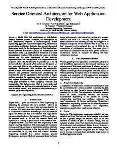
Process Modelling. An expert or process designer models the process and augments it with necessary temporal information. Figure 1 visualizes a workflow

An Architecture for Proactive Timed Web Service Compositions Start

4 A

4 B

End

3 C

deadline= 13 deadline

B.st A.d

325

B.d C.d time

0

1

2

3

4 B.eps

5

6

7

8

9

10 11 B.lae

12

13

Fig. 1. Valid Execution Interval of Activity B

consisting of three activities executed in sequence. Explicit time properties are the estimated duration of activities in basic time units, which are A.d = 4, B.d = 4 and C.d = 3 and a deadline of δ = 13, stating that the overall workflow execution must not exceed 13 time units.1 Calculation of the Timed Graph. The output of this phase is called Timed Graph which augments the process model with valid execution intervals for each node or activity. The time line in Figure 1 shows these execution intervals for activity B. A relative time model is used, where 0 denotes the start time of the process. All other points in time are declared or calculated relative to this start time [16]. Based on this information the valid execution interval for activity B is calculated as follows: an activity must not start until all predecessors are finished (since we assume that there is no delay between activities), therefore the earliest possible time B may start is determined by the sum of predecessor durations: B.eps = 4. To take the deadline of 13, into account, the point of view has to be reversed, now starting from the end of the workflow. By subtracting the durations of succeeding activities from the deadline, the latest allowed end B.lae of activity B is determined: B.lae = 13 − 3 = 10. In the figure one can also spot the time span B.st, which depicts the slack or buffer time; this time may be consumed by B without endangering the deadline.2 The EPS-values for all activities are calculated in a forward pass and the LAE-values in a backward pass, as described in e.g. [14], where along with simple sequences also conditional, alternative and parallel execution structures are considered, as well as upper and lower bound constraints. In order to cope with run time uncertainties like varying execution durations and branching and looping behavior (treatment of blocked loops) a stochastic model was introduced in [11,12], where each time value is represented as histogram, which allows statements for certain confidence thresholds. 1

2

Although it can not be recommended to represent durations with simple scalar time values, we will still use this representation to reduce the complexity of explanations. In the prototypical implementation we used the probabilistic model presented in e.g. [11,12], where time values are represented as histograms, which allow more differentiated statements about the temporal status of a process. Slack time is produced by relaxed deadlines or on shorter branches of parallel structures.

326

2.2

J. Eder, H. Pichler, and S.Vielgut

Process Instantiation

The workflow engine starts, controls and terminates the control flow of process instances. When starting a new process instance the time manager has to load the according timed graph and adjust it to the current date and time. This step is called Calendar Mapping, which in its simplest form just adds the current date and time to each EPS and LAE-value in the timed graph. 2.3

Process Run Time

Monitor State of Execution. During process execution a time management component must map each currently executed activity with its counterpart-node in the timed graph. Predictive Time Management. The prediction component has several functions: it may be used to predict the rest execution time of the process [11] or to forecast the arrival time of future tasks for certain workflow participants (based on EPS-values) [9]. For this paper the most important feature is the prediction of eventually arising future deadline violations based on LAE-values. E.g. if B ends later than 13 (time units after the start of the process) one can state that it is likely that the deadline will be violated after finishing C. In contrast to reactive time management, which solely reacts on constraint violations that already occurred, predictive time management forecasts violations and enables the system to initiate evasive actions [14]. Proactive Time Management. Proactive time management will be started after the prediction of violations. Its purpose is to trigger appropriate evasive actions. Consider our running example: before C is even started according evasive actions can be invoked in order to hold the deadline, for instance exchanging activity C with an alternative shorter activity C  . We claim that early prediction of time constraint violations and their pro-active treatment saves costs and therefor increases the quality of service [12].

3

Architecture for Timed Web Service Compositions

Figure 2 proposes an architecture for a BEPL-based web service environment which enables proactive time management. The architecture consists of the Process Engine and the Time Managers Build Time and Run Time components. Time Manager Build Time Components 1. The Parser loads the BPEL-definition, parses it and generates an according Process Graph. 2. The Data Collector augments the graph with additional temporal process information, like expected activity durations and time constraints.

An Architecture for Proactive Timed Web Service Compositions

Process Graph

Extended Graph

Timed Graph

1hour

Time Manager - Build Time Components

9hours

Parser

Data Collector

2hours

327

1hour 5hours

9hours

2hours

5hours

Timed Graph Calculator

Duration, Branching, Constraints

Process Definition BPEL

Start Process

3d Party QoS

History

Model DB

Experts Instance Models (Calendar Mapped)

Log Events

Instance 1

Events

Instance Model Mapper

Intervention

Proaction

Instance Graph 3

Instance Graph 1

Instance 2 Instance 3

Prediction Process Engine

Instance Graph 2

Time Manager Run Time Components

Temporal Status

User, Administrator

Fig. 2. Time Manager Architecture

3. The resulting Extended Graph is fed into the Timed Graph Calculator, which generates the Timed Graph. 4. And finally the Timed Graph is stored in the Model Database. Process Engine 1. The BPEL-Process Engine starts new process instances and controls their execution (communication with web services). 2. During the execution of process instances certain events, like start or termination of process activities, are signaled to the run time component of the time manager. 3. In order to avoid possible future violations of time constraints the process engine reacts to intervention signals from the time manager. Time Manager Run Time Components 1. When a process is started by the process engine an according signal will be sent to the time manager. 2. The Instance-Model Mapper loads the according timed graph from the model database and generates a calendar-mapped copy, called Timed Instance Graph, for the process instance.

328

J. Eder, H. Pichler, and S.Vielgut

3. Each time an activity of the process instance starts or ends an according signal will be sent to the instance-model mapper. 4. The Prediction Component periodically checks the temporal status of the instance and raises an exception if time constraints are likely to be violated. Additionally it provides an interface to monitor the temporal status of each process instance (e.g. likelihood of deadline violations, expected remaining execution time) which may be accessed by users, service requestors or process administrators. 5. In this case the Proactive Component jumps into action, tries to find an alternative (shorter) execution plans in order to prevent a future deadline violation, and sends according intervention instructions to the process engine. The current status of the prototypical implementation and research tasks is as follows: the build time components are completed and now we focus on the proactive part, namely service exchange algorithms. For the Java-based implementation of the prototype the following tools and technologies were used: Oracle BPEL Server, Eclipse + Oracle BPEL Designer Plugin, Apache Tomcat, Axis Soap Engine and the Xerces2 XML-Parser [22].

4 4.1

Build Time Components Parser: Generating the Process Graph

The first step is to parse the web services-based process definition in order to generate a graph-based process representation, which is necessary for the time management calculations performed later. In a service oriented architecture enterprizes or their applications respectively communicate via loosely coupled web services, which are described by standards like the Web Service Description Language (WSDL) [24,1]. As these services do very often not operate in isolation, but in the context of a business process, a description language must be used to define e.g. the data flow between and the execution order of web services. The Process Execution Language for Web Services (BPEL, BPELWS) is such a language [4,1]. Note that we concentrate on executable business processes, which require, similar to processes in workflow systems, a central process execution engine that enacts and controls process instances. In a services-based scenario the engine communicates either synchronously or asynchronously with external web services, which form the steps in a business process. BPEL provides several base activities to communicate with web services, like invoke, receive or reply. Additionally it provides so called structural activities to define the control flow between base activities, like sequence, switch, flow or while. As BPEL originates from block-structured (XLANG) and activity diagram-based (WSFL) languages the control flow of a BPEL process definition can be represented a directed graph with control nodes [3]. Therefore the transformation of a BPEL-definition into a process graph poses no further problems for the Parser.

An Architecture for Proactive Timed Web Service Compositions

4.2

329

Data Collector: Generating the Extended Graph

In many workflow systems activities have additional attributes holding expected execution durations, which are mainly used for simulation and process reengineering purposes [23,18]. Additionally time constraints can be defined to e.g. enable the enforcement of organizational rules. Extended Information. In addition to the control flow structure defined in the process definition, time management algorithms need the following information to calculate their temporal models: – Response Time: Each activity must be augmented with the expected duration, or since we talk about services, call it response time. – Time Constraints: Several types of time constraints exist. An overall process deadline is a time constraint which restricts the execution duration of the whole process. A lower bound constraint is defined between a source and a target activity which are not necessarily adjacent in the graph. It defines a minimum time that must pass after finishing the source activity, before the target activity is allowed to start. An an Upper Bound Constraint defines a maximum time that is allowed to pass between the source and the target activity. Data Sources. The function of the Data Collector is to gather this additional information and extend the process graph with it, where the following data sources may be accessed: – Experts: Information stemming from organizational rules, like time constraints, must be introduced by expert process modelers. If no other sources are available experts may additionally make estimations about service response times. – Process History: If knowledge about past process execution exists, response times can also be extracted from the process history. The process history (or process log) stores events which occur during process execution, for instance the start or end of activities, along with according time stamps. – Third Party: Sometimes the extraction of response times tends to be a problem, especially in flexible environments where autonomous web services, accessed by the composition, are frequently changing. For these cases response times could also be stored and administered by trusted third parties, which offer an interface to access statistics, similar to or as an extension of a (Web) Service Level Agreement-architecture [7,15]. In order to automate data collection we extended the original WSDL of each service contained in the composition with a time management interface which provides methods (e.g. getResponseTime) to access extended data. The (hidden) implementation of these methods provides access to one of the above mentioned types of the data sources and can be uniformly accessed via the web service interface. The implementation may for instance be a query to an experts database or forwarding the request to a third party interface.

330

4.3

J. Eder, H. Pichler, and S.Vielgut

Timed Graph Calculator

As BPEL-definitions can be represented as graphs and all possible structural activities are supported by according control flow structures, as addressed in e.g. [14,11,12], it already seems that time management algorithms as explained in Section 2 can be applied without further adaptations. Unfortunately existing workflow time management approaches are based on one assumption: activities are interpreted as basic execution units which must be finished in order to proceed with workflow execution. But in Web Service scenarios external services, applications or sub-processes are started, using a blocking (synchronous) or nonblocking (asynchronous) communication model. To enable our time management algorithms to cope with these models it was necessary to examine the structure of communication scenarios and how they affect EPS- and LAE-values. Recent publications on web service communication and web service composition, e.g. [1,20,3], already identified several basic synchronous and asynchronous communication patterns, which we had to consider in our time management calculation algorithms. A detailed description of how to handle each pattern can be found in [13]. Synchronous Patterns. In a synchronous or blocking model the requester waits for the response of the provider before it continues execution. The advantage of this model is its simplicity, as the process state does not change until the response has been received. The obvious disadvantage is that blocking the execution of the main process, especially when long running external processes are involved, increases its execution duration tremendously. For synchronous communication patterns no special mapping is necessary since after the invocation of an external service process execution will be blocked until the response is received, which is exactly the behavior of so called atomic activities in workflow systems. Asynchronous Patterns. Although synchronous communication is appropriate in many situations it may be suboptimal when long-running external services or sub-processes are called. In an asynchronous or non-blocking model the main process sends a request to the provider and continues execution without delay. At a later point in time it receives a response (callback) from the provider, which of course implies that the main process contains an activity which waits to receive this response. Asynchronous communication loosely couples sender and receiver. This accelerates process execution and compensates communication problems (e.g. network problems). But for time management it poses a problem as visualized on the left-hand side in Figure 3: a web service composition consists of a sequence of activities, where the first one invokes an external web service, which itself hides a process. As the communication is non-blocking, the process engine continues execution with succeeding activities (which may for instance be blocking calls to other services). The last activity receive synchronizes the external web service, as it waits for the response message.3 3

For details on callbacks and how response messages are correlated to their appropriate process instances, e.g. using correlation-ids, we refer to [1].

An Architecture for Proactive Timed Web Service Compositions

Deadline: 10

Composition invoke request

5 B

4 C

9 X

3 Y

External Web Service

receive response

Deadline: 10

Composition invoke

331

5 B

4 C

receive

lbc: 12

Response Time: 12

Fig. 3. Invocation of an External Web Service

Assuming that the duration of invoke and receive is 0, one could be tempted to state that the overall execution duration of the composition is 9, which is less than the deadline of 10. But of course it is necessary to consider the response time of the invoked service which is 12, therefore the deadline will be violated. One can see that the time span between invoke and receive is determined by the maximum of the duration of the regular path and the duration of the external service. Please note that in this scenario an external web service with a response time less than 9 hours (which is the sum of durations of B and D) would have had no effect on the execution duration of the workflow and the execution intervals of its activities, as in this case the longer regular path via B and D would determine these values. In order to calculate the timed graph we have to introduce a temporal relationship between the invoking and the receiving activity, where asynchronous communication with a web service can be easily mapped to a lower bound constraint (see right-hand side in Figure 3). The forward and backward calculations may then be performed as explained in [14], which states that for activities which are connected by a lower bound constraint the longest path determines the according time intervals. A required prerequisite is to connect the invoke and the adhering receive activity with a lower bound. This can be automated during parsing if the BPEL-definition contains according partner links and bindings [1,22]. Note also that since the invoked service may reside anywhere its structure will be unknown and it must therefore be treated as a black box. The only knowledge required is its expected response time which can for instance be determined by retrieving the QoS-information on this service from a trusted third party. 4.4

Model Database

At the last step of the build time phase the timed graph must be stored in the Model Database. The model database holds a timed graph for each time-managed process. The model is stored as an XML-representation of the timed graph model, which consists of nodes, edges and temporal relations. Nodes hold temporal information (EP- and LA-values) and a mapping to the WSDL-specification and according partner links. Edges connect nodes and temporal relations represent time constraints like lower bounds.

332

5 5.1

J. Eder, H. Pichler, and S.Vielgut

Run Time Components Instance-Model Mapper

To monitor the progress of a process instance and its temporal status the time manager needs to be notified of certain events, which are: start of a process or activity, end of a process or activity and the abnormal termination of a process. Each of these events must be signaled to the Instance-Model Mapper which reacts as follows: Start Process. The mapper generates a copy, called Timed Instance Graph, of the according timed graph which it loads from the model database. Afterwards each EPS and LAE-value in this graph is mapped to the real calendar, which means that the current date and time is added. Consider the example from Section 2: in the original model the valid execution interval is defined as relative distance to the start time 0 of the process, e.g. B.eps = 4 and B.lae = 10. Assuming that the time unit used is hours and the (current) time at the start of the process is M onday 1st, 8am the interval in the instance graph will be calendarmapped as follows: B.eps = M onday 1st, 12am and B.lae = M onday 1st, 6pm. Of course this applies for the intervals of all activities the timed instance graph, as well as for the overall deadline which is mapped to M onday 1st, 9pm. Additionally the execution pointer is initialized with a reference to the start activity (in the timed instance graph). Start Activity, End Activity. The mapper updates the execution pointer such that it references the currently executed activity (in the timed instance graph). End Process, Cancel Process, Termination Due to Failure. The mapper discards the timed instance graph. 5.2

Predictive Time Manager

This component checks periodically and on arrival of certain events if the current execution status is likely to cause time constraint violations in the future. E.g. activity B finishes at time M onday 1st, 7pm and the process enginge signals end of activity B to the time manager. By comparing the actual end time of B with its latest allowed end time B.lae = 6pm the time manager finds out that a deadline violation is likely to occur. Actually it predicts that after the execution of C the process will most likely finish at 10pm, which is 1 hour after the calendar-mapped deadline, and therefore 1 hour to late. It raises an according exception which must be handled by the Proactive Time Manager. As an additional feature the prediction componentent provides an interface to monitor the temporal information and status of each process instance which

An Architecture for Proactive Timed Web Service Compositions

333

may be accessed by users, service requestors or process administrators. Service requestors might for instance be interested in the expected completion date/time of a certain process instance. Process administrators might want to know the temporal status of an instance. In [14] the traffic light model was introduced, which proposes different temporal states that are set according to the likelihood of a deadline violation: green (everything ok), yellow (problems possible) and red (violation most likely to occur). 5.3

Proactive Time Manager

When this component catches an exception the process is already late, which means that the rest of the process must be sped-up in order to reach the given deadline. We just started to research methods to exchange services with faster alternatives. Of course it is possible that these alternative services have some drawbacks (which is the reason that they were not chosen in the first place), e.g. they might be more expensive. The first input parameter for such an algorithm is the amount of time that must be saved; consider the running example: activity B is late by one hour, therefore the succeeding activities must be accelerated by at least one hour, in order to meet the deadline. Additionally such an algorithm will need to know which services are exchangeable, along with a set of alternative services for each of them (we plan to realize a static approach in the prototypical implementation). The next step is the generation of an alternative constraintviolation free process execution plan. This is not so straightforward as it seems at first glance. E.g. exchanging a service with a shorter alternative might not affect the execution duration of the process at all, if it for example resides on a path where still slack time is available. Additionally it might be necessary to exchange more than one service. However, in every case a partial recalculation of the timed instance graph will be necessary. Finally the process engine must be informed about the changes it has to apply on the (still running) process instance.

6

Current Work, Future Work and Conclusions

The prediction and proactive avoidance of deadline violations decreases costs of processes and increases their quality of service. In this paper we proposed a time manager architecture for web service composition environments, showed how to apply workflow time management algorithms, explained in detail how build time and some run time components work and provided some ideas of how to solve still open run time problems. To prove the feasibility of our concepts we implement a web services-based time management framework, where we currently concentrate on the run time aspects, especially on repair and service exchange algorithms. Additionally we examine the applicability of proactive time management features on other quantifiable quality dimensions, like cost or reliability. The integration of proactive repair mechanisms into process automation environments is subject of ongoing research.

334

J. Eder, H. Pichler, and S.Vielgut

References 1. G. Alonso, F. Casati, H. Kuno, V. Machiraju. Web Services: Concepts, Architectures and Applications. Springer Verlag, ISBN 3-540-44008-9, 2005. 2. W. M. P. van der Aalst and H. A. Reijers. Analysis of discrete-time stochastic petrinets. In Statistica Neerlandica, Journal of the Netherlands Society for Statistics and Operations Research, Volume 58 Issue 2, 2003. 3. Petia Wohed and Wil M.P. van der Aalst and Marlon Dumas and Arthur H.M. ter Hofstede. Pattern Based Analysis of BPEL4WS. QUT Technical report, FIT-TR2002-04, Queensland University of Technology, Brisbane, 2002. 4. Business Process Execution Language for Web Services Version 1.1 - BPEL4WS Specification. BEA, IBM, Microsoft, SAP and Siebel, 2004. 5. G. Baggio and J. Wainer and C. A. Ellis. Applying Scheduling Techniques to Minimize the Number of Late Jobs in Workflow Systems. In Proc. of the 2004 ACM Symposium on Applied Computing (SAC). ACM Press, 2004. 6. C. Combi and G. Pozzi. Temporal conceptual modelling of workflows. LNCS 2813. Springer, 2003. 7. J. Cardoso and A. Sheth and J. Miller. Workflow Quality of Service. Proceedings of the International Conference on Integration and Modeling Technology and International Enterprise Modeling Conference (IEIMT/IEMC’02), Kluwer Publishers, 2002. 8. P. Dadam and M. Reichert. The ADEPT WfMS Project at the University of Ulm. In Proc. of the 1st European Workshop on Workflow and Process Management (WPM’98). Swiss Federal Institute of Technology (ETH), 1998. 9. J. Eder, W. Gruber, M. Ninaus, and H. Pichler. Personal Scheduling for Workflow Systems. LNCS 2678, Springer Verlag, 2003. 10. J. Eder and E. Panagos. Managing Time in Workflow Systems. Workflow Handbook 2001. Future Strategies Inc. Publ. in association with Workflow Management Coalition (WfMC), 2001. 11. J. Eder and H. Pichler. Duration Histograms for Workflow Systems. In Proc. of the Conf. on Engineering Information Systems in the Internet Context 2002, Kluwer Academic Publishers, 2002. 12. J. Eder and H. Pichler. Probabilistic Workflow Management. Technical report, Universitt Klagenfurt, Institut fr Informatik Systeme, 2005. 13. J. Eder and H. Pichler. Avoidance of Deadline Violations for Interorganizational Business Processes. Seventh International Baltic Conference on Databases and Information Systems DB&IS, Technika, 2006. 14. J. Eder, E. Panagos, and M. Rabinovich. Time constraints in workflow systems. LNCS 1626. Springer, 1999. 15. M. Gillmann, G. Weikum, and W. Wonner. Workflow management with service quality guarantees. In Proceedings of the 2002 ACM SIGMOD International Conference on Management of Data. ACM Press, 2002. 16. H. Jasper and O. Zukunft. Time Issues in Advanced Workflow Management Applications of Active Databases. In Proc. of the 1st International Workshop on Active and Real-Time Database Systems. Workshops in Computing, 1995. 17. B. Kiepuszewski, A. ter Hofstede, C. Bussler. On Structured Workflow Modeling. In: Proceedings of the 12th Conference on Advanced Information Systems Engineering (CAISE). Stockholm, Sweden, June 2000. 18. M. Laguna and J. Marklund. Business Process Modeling, Simulation and Design. ISBN 0-13-091519-X. Pearson Prentice Hall, 2005.

An Architecture for Proactive Timed Web Service Compositions

335

19. O. Marjanovic and M. Orlowska. On modeling and verification of temporal constraints in production workflows. Knowledge and Information Systems, 1(2), 1999. 20. E. Newcomer. Understanding Web Services. Verlag: Addison-Wesley, ISBN 0-20175081-3, 2002. 21. E. Panagos and M. Rabinovich. Predictive workflow management. In Proc. of the 3rd Int. Workshop on Next Generation Information Technologies and Systems, Neve Ilan, ISRAEL, 1997. 22. S. Vielgut. Time Management in Web Service Orchestrations. Master Thesis, University of Klagenfurt, 2005. 23. Workflow Process Definition Interface. A Workflow Management Coalition Specification. Document number WFMC-TC-1025, 2002. 24. E. Christensen and F. Curbera and G. Mereditih and S. Weerawarana Web Service Definition Language 1.1 - WSDL Specification IBM, Microsoft, 2001.