Edsger W. Dijkstra and C. S. Scholten. Termination detection for diffusing computations. Info. Proc. Lett., ll(l):l-4, August 1980. 10. Yogen K. Dalal y Robert M.
An Architecture to Connect Disjoint Multimedia Networks Based on node’s Capacity Jaime Lloret, Juan R. Diaz, Jose M. Jimenez, Fernando Boronat Department of Communications, Polytechnic University of Valencia Camino Vera s/n, Valencia, Spain {jlloret, juadasan, jojiher, fboronat}@dcom.upv.es
Abstract. TCP/IP protocol suite allows building multimedia networks of nodes according to nodes’ content sharing. Some of them have different types of protocols (some examples given in unstructured P2P file-sharing networks are Gnutella 2, FastTrack, OpenNap, eDonkey and so on). This paper proposes a new protocol to connect disjoint multimedia networks using the same resource or content sharing to allow multimedia content distribution. We show how nodes connect with nodes from other multimedia networks based on nodes’ capacity. The system is scalable and fault-tolerant. The designed protocol, its mathematical model, the messages developed and their bandwidth cost are described. The architecture has been developed to be applied in multiple types of multimedia networks (P2P file-sharing, CDNs and so on). We have developed a general-purpose application tool with all designed features. Results show the number of octets, the number of messages and the number of broadcasts sent through the network when the protocol is running. Keywords: P2P, Architecture, content distribution, groups.
1 Introduction and Motivation Today, the grouping of nodes in multimedia networks is more and more extended in Internet. They could be grouped based on content sharing, or according to similar characteristics, functionalities or even social trends. Many researchers try to find the best application layer protocol and architecture to organize and join nodes in a multimedia network [1], [2]. Once they are grouped, data are kept inside the multimedia network and only nodes joined to the network can download or stream data shared inside. Let’s consider a set of autonomous multimedia networks. All nodes in the multimedia networks run their application layer protocol. Each node shares or streams content using the application layer protocol. All application layer protocols can be translated to other protocols and they are not encrypted using signatures or private keys. An interconnection system over those multimedia networks will give some benefits for the whole system such as: (1) Content availability will be increased. (2) It will facilitate data or content replication in other multimedia networks. (3) When a new multimedia network is added to the system, existing
desktop applications will not be changed. (4) Network measurements could be taken from any multimedia network. (5) Desktop applications could search and download from every multimedia network using only one open service. Once the interconnection system is working, when a node looks for some data, first it will try to get it from its network. In case of no result, the search could be sent to other networks. If it is found, the data can be downloaded or transferred to the first network. Once the node has that data, it will act as a cache for its network sharing the data. The existing systems are based on a desktop application which knows several protocols and is able to join several networks. Examples are Shareaza [3], MLDonkey [4], giFT [5], Morpheus [6] and cP2Pc [7]. To use those solutions, taking “search for a file” as an example, the user has to be permanently connected to all networks. The computer that joins all networks needs a lot of processing capacity. In addition, if a new P2P file sharing network is developed, a new plugin is required to support the new architecture; and, all users will have to update their clients to join the new network. On the other hand, this solution allows a node to join several multimedia networks, but those networks will not be interconnected. This paper is structured as follows. Section 2 describes our proposal architecture, the mathematical model, its components and its parameters. Section 3 explains the protocol and recovery mechanisms. Messages designed and their bandwidth are shown in section 4. Section 5 shows an application tool developed using our protocol and measurements taken for different events. Related works and differences with them are explained in section 6. Finally, section 7 gives the conclusions.
2 Mathematical description When a node joins the proposed architecture, it has the following parameters previously defined: (1) A multimedia network identifier (networkID). All nodes in the same network have the same networkID. (2) Upstream and downstream bandwidth. (3) Maximum number (Max_num) of supported connections from other nodes. (4) Maximum % of CPU load used for joining the architecture by the desktop application (Max_load). (4) What kind of content or data shared are in its network. Nodes could have 2 types of roles. Nodes with first role (Dnodes) establish connections with Dnodes from other networks as a hub-and-spoke. Dnodes are used to send searches and data transfers between networks. Nodes with second role (Onodes) are used to organize connections between Dnodes from different networks. For scalability reasons, Onodes could have 2 roles: to organize Dnodes in zones (level-1 Onodes) and to have connections with Onodes from other networks (level-2 Onodes). This paper considers only one type of Onode which has both roles. More details about an interconnection system using two levels of Onodes are shown in [8]. First node, from a new multimedia network, will be Onode and Dnode. New nodes will be Dnodes, but they could acquire higher roles because of some parameters discussed later. A node identifier (nodeID) is assigned sequentially, using a timestamp by the Onode, to every new node. Then, the new node calculates 2 parameters: - δ parameter. It depends on the node bandwidth and its age in the system. It is used to know which node is the best one to have a higher role. A node with
higher bandwidth and older is preferred, so it will have higher δ. The number of nodes needed to promote a node depends on the type of multimedia network. Equation 1 gives δ parameter. δ = ( BWup + BWdown )·K1 + (32 − age)·K 2
-
(1)
Where age=log2(nodeID), so age varies from 0 to 32. K1 and K2 adjust the weigh of the bandwidth and the node’s age. We can see that older nodes will have more architecture functionalities than new ones unless they have low bandwidth. Nodes with high bandwidth and relatively new ones could have higher δ values. λ parameter. It represents the node capacity, and depends on: the node’s upstream and downstream bandwidth (in Kbps), its number of available connections (Available_Con) and its maximum number of connections (Max_Con) and its % of available load. It is used to determine the best node. It is given in equation 2. ⎡ (BWup + BWdown ) ⎤ int ⎢ + 1⎥· Available _ Con ⋅ (100 − load ) + K 3 256 ⎦ λ= ⎣ Max _ Con
(2)
Where 0 ≤ Available_Con ≤ Max_Con. Load varies from 0 to 100. A load of 100% indicates the node is overloaded. K3 give λ values different from 0 in case of a 100% load or Available_Con=0. Dnodes take the Onode election based on δ parameter. There could be more than one Onode per network. It depends on the number of Dnodes in the multimedia network. From a practical point of view, we can consider a big multimedia network, which is split into smaller zones (different multimedia networks). Every node has 5 parameters (networkID, nodeID, δ, λ, role) that characterize the node. The following describes how every node works depending on its role. 2.1 Onodes organization We have chosen the routing algorithm SPF to route searches for providing Dnodes adjacencies. The cost of the ith-Onode (Ci) is based on the inverse of the ith-Onode λ parameter. It is given by equation 3. C=
K4 λ
(3)
With K4=103, we obtain C values higher than 1 for λ values given in equation 2. Nodes with Available_Con=0 and/or load=100 will give C=32. The metric, to know which is the best path to reach a destination, is based on the number of hops to the destination and the cost of the Onodes involved in that path. It is given by equation 4. n
Metric = ∑ C i
(4)
i =1
Where Ci is the ith node virtual-link cost and n is the number of hops to a destination.
Given G = (V, C, E), an Onodes network, where V is a set of Onodes V= {0, 1,…, n}, C is a set of costs (Ci is the cost of the ith-Onode and Ci≠0 ∀ i-Onode) and E is a set of their connections. Let D=[Mij] be the metric matrix, where Mij is the sum of the costs of the Onodes between vi and vj. We assume Mii=0 ∀ vi, i.e., the metric is 0 when the source Onode is the destination. On the other hand, vi and vj ∈ V, and Mij =∞ if there is not any connection between vi y vj. So, supposing n hops between vi and vj. The Onode Mij matrix is given by equation 5. n
When ∃ a path between vi and vj ⎧ min( ∑ cos t (v k )) ⎪ k =1 Mij = ⎨ (5) ⎪ ⎩ ∞ In other case In order to calculate the number of messages sent by the whole network, we consider that the ith-Onode has CN(i) neighbours, where CN(i)={j |{i,j} ∈ E}. On the other hand, every Onode calculates Mij ∀ j and builds its topological using Dijkstra algorithm. Then, every i Onode sends its topological database to its CN(i) neighbours and they to their neighbours until the network converges. Finally, all Onodes can calculate their lower metric paths to the rest of the Onodes, i.e., Mij [9]. When there is a fixed topology where all Onodes have to calculate the lower metric path to the others, the number of messages sent by every Onode is O(V·D+E), where D is the network diameter. In the proposed system, Onodes can join and leave the topology any time, so the metric matrix is built as the Onodes join and leave the topology. When a new Onode joins the system, it will build its topological database and its neighbours will send the update to its neighbours except to the new Onode. Neighbour Onodes will send the update to all their neighbours except to the one from who has received the update. In addition, the update is sent only if the update is received from the Onode in the lower metric path to the one who has started the update (Reverse Path Forwarding [10]). Taking into account considerations aforementioned, given n=|V| Onodes in the whole network, m=|E| the number of connections in the network, d the diameter of the network and supposing that the ith-Onode has CN(i) neighbours, we obtain results shown in table 1 (tp is the average propagation time). Table 1. Results for Onodes organization. Number of messages sent by an Onode because an update Number of updates sent in the whole network Time to converge
CN(i)-1 n d·tp
Metric
∑ λ (i )
Number of messages sent by an Onode because an update
CN(i)-1
n
1
i =1
2.2 Dnodes organization Given G = (V, λ, E) a network of nodes, where V is a set of Dnodes, λ is a set of capacities (λ(i) is the i-Dnode capacity and λ(i)≠0 ∀ i-Dnode) and E is a set of connections between Dnodes. Let k be a finite number of disjoint subsets of V, ∀ V=Union(Vk). Given a Dnode vki (Dnode i from the k subset), there is not any
connection between Dnodes from the same subsets (eki-kj=0 ∀ Vk). Every vki Dnode has a connection with one vri from other subset (r≠k). Let D=[Mki] be the capacity matrix, where Mki is the capacity of the i-Dnode from the k subset. Let’s suppose n=|V| and k the number of subsets of V, then we obtain equation 6. k
n = ∑ | Vk |
(6)
i =1
On the other hand, the number of connections m=|E| depends on the number of subsets (k), the number of Dnodes in each subset (km) and the number connections that a Dnode has with Dnodes from other subsets (we will suppose that a Dnode has k-1 connections). Equation 7 gives m value. m=
1 k k m k −1 ∑∑∑ vkm (l ) 2 i =1 j =1 l =1
(7)
Where vkm(l) is the l-connection from the m-Dnode from the k subset. Let’s suppose there are n multimedia networks and only one Onode per multimedia network. When a Dnode sends a request to its Onode, it broadcasts this request to all other Onodes, so, taking into account results from subsection B, there will be n messages. When this message arrives to the Onode from other network, it will elect its two connected Dnodes with higher λ and they acknowledge the message, so, it is needed 2 messages. Then, Dnodes from other networks will send a connection message to the requesting Dnodes and they confirm this connection, so it is needed 2 messages more (it is explained in section 3). This process is done in every network. The sum of all messages, when a Dnode requests adjacencies, is shown in equation 9. messages = 1+ 5·n
(9)
3 Protocol description and recovery algorithms When a Dnode joins the interconnection system, it sends a discovery message with its networkID to Onodes known in advance or by bootstrapping [11]. Only Onodes with the same networkID will reply with their λ parameter. Dnode will wait for a hold time and choose the Onode with highest λ. If there is no reply for a hold time, it will send a discovery message again. Next, Dnode sends a connection message to the elected Onode. This Onode will reply a welcome message with the nodeID assigned. Then, the Onode will add this information to its Dnodes’ table (it has all Dnodes in its area). Onodes use this table to know Dnode’s δ and λ parameters. Finally, Dnode will send keepalive messages periodically to the Onode. If an Onode does not receive a keepalive message from a Dnode for a dead time, it will erase this entry from its database. Steps explained can be seen in figure 1. First time a Dnode establishes a connection with an Onode, it will send to that Onode a requesting message to establish connections with Dnodes from all other networks. This message contains destination networkID, or a 0xFF value (broadcast), sender’s networkID, sender’s nodeID and its network layer address. When the Onode
receives the request, it will broadcast the message to all Onodes from other networks. The message is propagated using Reverse Path Forwarding Algorithm. Only Onodes from other networks will process the message. When an Onode receives this message, it will choose its two connected Dnodes with higher λ and it will send them a message informing they have to establish a connection with a Dnode from other network. This message contains the nodeID and the requesting Dnode’s network layer address. When these Dnodes receive that message, they will send a message to connect with the Dnode from the first network. When the connection is done, Dnodes from the second network will send a message to its Onode to inform they have established a connection with the requesting Dnode. If Onode does not receive this message for a hold time, it will send a new message to the next Dnode with highest λ. This process will be repeated until Onode receives both confirmations. When the requesting Dnode receives these connection messages, it will add Dnode with highest λ as its first neighbor and the second one as the backup. If the requesting Dnode does not receive any connection from other Dnode for dead time, it will send a requesting message again. Then, both Dnodes will send keepalive messages periodically. If a Dnode does not receive a keepalive message from the other Dnode for a dead time, it will erase this entry from its database. Every time a Dnode receives a search or data transfer for other networks, it looks up its Dnodes’ distribution table to know to which Dnode send the search or data. Figure 2 shows all steps explained. When an Onode receives a new networkID, it will send a message to all Dnodes in its zone. Subsequently, Dnodes will begin the process to request Dnodes from the new network. Dnode with highest δ will be the backup Onode and it will receive Onode backup data by incremental updates. This information is used in case of Onode failure. Onode sends keepalive messages to the backup Dnode periodically. When an Onode fails, backup Onode will check it because of the lack of keepalive messages for a dead time, so, it will start Onode functionalities using the backup information. When an Onode leaves the architecture voluntarily, it will send a message to the backup Dnode. The backup Dnode will send it an acknowledgement, and, when it receives the ack message, it will send a disconnection message to its neighbours and leave the architecture. Then, the Dnode that is the backup Onode starts Onode functionalities using the backup information. When a Dnode leaves the architecture voluntarily or fails down, Onode and adjacent Dnodes will ckeck it because they do not receive a keepalive message for a hold time. They will delete this entry from their Dnodes’ database and adjacent Dnodes will request a new Dnode for this network as explained in figure 2. Dnode
Several Onodes with the same networkID
Onodes with higher λ
Network 1 Dnode
DDB request
Wait
D discovery ACK D connect
Wait
Added to Dnodes’ Table
Welcome D Keepalive D
Network 2 Dnode
DDB request
D discovery
Wait
Network 2 Onode
Network 1 Onode
Keepalive reset to 0
Figure 1. Messages when a new Dnode joins the architecture.
Elected Dnode
DD connect DD Welcome Elected Dnode Ack
Keepalive reset to 0
Keepalive DD Keepalive DD
Figure 2. Messages to request Dnode’s connections.
4 Messages Bandwidth We have developed 31 messages for the interconnection system. They can be classified in 2 classes: (1) Fixed size messages. (2) Messages which size depends on the number of neighbours, the size of the topological database or the backup information (O neighbors, ODB, Backup O in table 2). In order to know the bandwidth consumed by those messages, let’s suppose they are sent using TCP/IP over Ethernet headers. The sum of those headers is 58 Bytes (as is has been considered for other P2P protocols [12]). We have considered that networkID, nodeID, λ and δ parameters use 32 bits and, in order to calculate messages that depends on other parameters, every Onode has 4 neighbors, Dnode’s table has 28 entries and the topological database may use the available TCP/IP over Ethernet payload. On the other hand, the limit of the TCP/IP over Ethernet payload is 1460 Bytes. Table II shows messages classified taking into account their number of bits. Figure 3 shows their bandwidth (we have used the numbers shown in table 2). Table 2. Message classification.
Bytes
1600
Nº Messages 1 D discovery, D connect y O request 2 D discovery ACK, Elected Dnode ACK, O discovery, Failed O, Failed O ACK, New O, Change nodeID, O disconnect, O conversion. 3 New Network, O discovery ACK, O connect. 4 Welcome D, Keepalive D, DDB Request, DD connect, Welcome DD, Keepalive DD, Keepalive O, O reply. 5 Elected Dnode, Welcome O, O replace. 6 O neighbors 7 ODB 8 Backup O
1400 1200 1000 800 600 400 200 0 1
2
3
4
5
6
7
8 Messages
Figure 3. Messages bandwidth consumption.
Messages with higher bandwidth are the ones that send the topological database and the backup information. Because of it, we have designed the system in such a way that these are only sent when changes take place. First time, both messages send the whole information, next times only updates are sent.
5 Measurements We have developed a desktop application tool, using Java programming, to run and test the designed protocol. We have programmed Dnode and Onode functionalities. The application allows us to choose the multimedia network to be connected with. We can configure the type of files or data to download. We can vary some parameters for δ and λ calculation and the maximum number of connections, maximum CPU load, upstream and downstream bandwidth, keepalive time and so on. We have used 24 Intel ® Celeron computers (2 GHz, 256 RAM) with Windows 2000 Professional © OS to know the protocol bandwidth consumption. They were connected to a Cisco Catalyst 2950T-24 Switch over 100BaseT link. One port was configured in a monitor mode (receives the same frames as all other ports) to be able to capture data using a sniffer application. We have tested three scenarios:
1. First scenario has only one group. It has only one Onode and there are 23 Dnodes in the group. We began to take measurements before we started the Onode. 2. Second scenario has two groups. Every group has one Onode. There are 11 Dnodes in each group. We began to take measurements before we started 1st Onode. We started a Onode from 1st group, 20 seconds later we started a Onode from the 2nd group, 20 seconds later we started 11 Dnodes from the 1st group and 20 seconds later we started 11 Dnodes from the 2nd group. 3. Third scenario has three groups. Every group has one Onode. There are 7 Dnodes each group. We began to take measurements before we started the Onodes. We started a Onode from 1st group, 10 seconds later we started 7 Dnodes from the 1st group, 10 seconds later, we started a Onode from the 2nd group, 10 seconds later, we started 7 Dnodes from the 2nd group, 10 seconds later, we started a Onode from the 3rd group, finally, 10 seconds later, we started 7 Dnodes from the 3rd group. Figure 5 shows the bandwidth consumed inside one group (1st scenario). There are some peaks because of the sum of joining discovery and keepalive messages (every 60 seconds) between Dnodes and the Onode. There are also DDB Request messages from Dnodes to other groups. Figure 6 shows the number of messages per second sent in the 1st scenario. Figure 7 shows the bandwidth consumed in the 2nd scenario. First peak (around 1 minute) shows when we joined 11 Dnodes from the 2nd group. Since this point, the number of octets in the network is higher because of keepalive messages. Figure 8 shows the number of messages per second sent in the 2nd scenario. Figure 9 shows the bandwidth consumed in the 3rd scenario. First peak (around 30 seconds) shows when we joined 7 Dnodes from the 2nd group. Once the 3rd group is started the bandwidth consumed is higher, but peaks are just bit higher than other scenarios. Figure 10 shows the number of messages per second in the 3rd scenario. Octets
Packe ts
14000
140
12000
120
10000
100
8000
80
6000
60
4000
40
2000
20
0 0:00
0:30
1:00
1:30
2:00
2:30
3:00
3:30
4:00
4:30 Time
0 0:00
Figure 5. 1st scenario bandwidth.
0:30
1:00
1:30
2:00
2:30
3:00
3:30
4:00 Time
Figure 8. 2nd scenario # of messages. Octets
Packe ts 120 100 80 60 40 20 0 0:00
0:30
1:00
1:30
2:00
2:30
3:00
3:30
4:00 Time
20000 18000 16000 14000 12000 10000 8000 6000 4000 2000 0 0:00
st
0:30
1:00
1:30
2:00
2:30
3:00
3:30
4:00
4:30 Time
rd
Figure 6. 1 scenario # of messages.
Figure 9. 3 scenario bandwidth.
Octets
Packets
16000
140
14000
120
12000
100
10000
80
8000 60
6000
40
4000
20
2000 0 0:00
0:30
1:00
1:30
nd
2:00
2:30
3:00
3:30
4:00
Figure 7. 2 scenario bandwidth.
4:30 Time
0 0:00
0:30
1:00
1:30
rd
2:00
2:30
3:00
3:30
Figure 10. 3 scenario # of messages.
4:00 Time
7 Related Works A. Wierzbicki et al. presented Rhubarb [13] in 2002. Rhubarb organizes nodes in a virtual network, allowing connections across firewalls/NAT, and efficient broadcasting. The nodes could be active or passive. This system has only one coordinator per group and coordinators could be grouped in groups in a hierarchy. The system uses a proxy coordinator, an active node outside the network, and Rhubarb nodes inside the network make a permanent TCP connection to the proxy coordinator, which is renewed if it is broken by the firewall or NAT. If a node from outside the network wishes to communicate with a node that is inside, it sends a connection request to the proxy coordinator, who forwards the request to the node inside the network. Rhubarb uses a three-level hierarchy of groups, may be sufficient to support a million nodes but when there are several millions of nodes in the network it could not be enough, so it suffers from scalability problems. On the other hand, all nodes need to know the IP of the proxy coordinator nodes to establish connections with nodes from other virtual networks. Z. Xiang et al. presented a Peer-to-Peer Based Multimedia Distribution Service [14] in 2004. The paper proposes a topology-aware overlay in which nearby hosts or peers self-organize into application groups. End hosts with in the same group have similar network conditions and can easily collaborate with each other to achieve QoS awareness. When a node in this architecture wants to communicate with a node from other group, the information is routed through several groups until it arrives to the destination. In our proposal, when a Dnode wants to communicate with a particular node from other group, it sends the information to the adjacent Dnode from that group which will contact with the node of that group, so there will be fewer hops to reach a destination (Onodes’ network is used to organize Dnodes’ connections only).
8 Conclusions We have presented a protocol to join multimedia networks that are sharing the same type of resources or content. It is based on two layers: Organization and distribution layer. First one joins all multimedia networks, organizes nodes in zones and helps to establish connections between Dnodes. Second one allows send searches and data transfers between networks. Once the connections are established, content or resource searches and data transfer could be done without using organization layer nodes. We have defined several parameters to know the best node to promote to higher layers or to connect with. The recovery algorithm when any type of node leaves the architecture or fails down is also described. We have shown that messages with more bandwidth are the backup message and the one which sends the topological database, so, they are maintained by incremental updates and we have designed taking into account that only first message will have all information. Measurements taken, for 2 and 3 multimedia networks interconnection, show the time needed when a Dnode fails. The protocol does not consume so much bandwidth. A multimedia network can be split into smaller zones to support a large number of nodes. The architecture proposed could be applied easily in that kind of networks.
This system has several adaptabilities such as CDNs [15] and railway sensor networks [16]. Now we are trying to interconnect P2P file-sharing networks using protocol signatures instead of the use of network identifiers. In future works we will adapt the architecture to sensor networks, using very short keepalive and dead time intervals, in order to have a fast recovery algorithm for critical systems.
References 1. E. K. Lua, J. Crowcroft, M. Pias, R. Sharma and S. Lim, “A Survey and Comparison of Peer to-Peer Overlay Network Schemes”. IEEE Communications Survey and Tutorial. 2004. 2. A. Vakali, G. Pallis, “Content delivery networks: status and trends”. Internet Computing, IEEE, Vol. 7, Issue 6. Pp. 68-74. 2003. 3. Shareaza, available at, http://www.shareaza.com/ 4. MLDonkey, at http://mldonkey.berlios.de/ 5. Morpheus, available at, http://www.morpheus.com 6. The giFT Project, at http://gift.sourceforge.net/ 7. Benno J. Overeinder, Etienne Posthumus, Frances M.T. Brazier. Integrating Peer-to-Peer Networking and Computing in the AgentScape Framework. Second International Conference on Peer-to-Peer Computing (P2P'02). September, 2002 8. J. Lloret, F. Boronat, C. Palau, M. Esteve, “Two Levels SPF-Based System to Interconnect Partially Decentralized P2P File Sharing Networks”, International Conference on Autonomic and Autonomous Systems International Conference on Networking and Services. 2005. 9. Edsger W. Dijkstra and C. S. Scholten. Termination detection for diffusing computations. Info. Proc. Lett., ll(l):l-4, August 1980. 10. Yogen K. Dalal y Robert M. Metcalfe, “Reverse path forwarding of broadcast packets”, Communications of the ACM. Volume 21, Issue 12 Pp: 1040 – 1048. 1978. 11. C. Cramer, K. Kutzner, and T. Fuhrmann. “Bootstrapping Locality-Aware P2P Networks”. The IEEE International Conference on Networks, Vol. 1. Pp. 357-361. 2004. 12. Beverly Yang and Hector Garcia-Molina. Improving Search in Peer-to-Peer Networks. Proceedings of the 22nd International Conference on Distributed Computing Systems (ICDCS’02). 2002. 13. Adam Wierzbicki, Robert Strzelecki, Daniel Świerczewski, Mariusz Znojek, Rhubarb: a Tool for Developing Scalable and Secure Peer-to-Peer Applications, Second IEEE International Conference on Peer-to-Peer Computing, P2P2002, Linköping, Sweden, 2002. 14. Xiang, Z., Zhang, Q., Zhu, W., Zhang Z., and Zhang Y.: Peer-to-Peer Based Multimedia Distribution Service, IEEE Transactions on Multimedia, Vol. 6. No.2, (2004) 15. J. Lloret, C. Palau, M. Esteve. “A New Architecture to Structure Connections between Content Delivery Servers Groups”. 15th IEEE High Performance Distributed Computing. June 2006. 16. J. Lloret, F. J. Sanchez, J. R. Diaz and J. M. Jimenez, “A fault-tolerant protocol for railway control systems”. 2nd Conference on Next Generation Internet Design and Engineering. April 2006.