An Automated Approach for Creating Workload ...

An Automated Approach for Creating Workload Models From Server Log Data Fredrik Abbors, Dragos Truscan, Tanwir Ahmad ˚ Akademi University, Joukahaisenkatu 3-5 A, Turku, Finland Department of Information Technologies, Abo {fredrik.abbors, dragos.truscan, tanwir.ahmad}@abo.fi

Keywords:

Workload model generation, Log file analysis, Performance testing, Probabilistic Timed Automata

Abstract:

We present a tool-supported approach for creating workload models from historical web access log data. The resulting workload models are stochastic, represented as Probabilistic Timed Automata (PTA), and describe how users interact with the system. Such models allow one to analyze different user profiles and to mimic real user behavior as closely as possible when generating workload. We provide an experiment to validate the approach.

1

INTRODUCTION

The primary idea in performance testing is to establish how well a system performs in terms of responsiveness, stability, resource utilization, etc, under a given synthetic workload. The synthetic workload is usually generated from some kind of workload profile either on-the-fly or pre-generated. However, Ferrari states that synthetic workload should mimic the expected workload as closely as possible (Ferrari, 1984), otherwise it is not possible to draw any reliable conclusions from the results. This means that if load is generated from a workload model, then the model must represent the real-world user behavior as closely as possible. In addition, Jain points out that one of the most common mistakes in load testing is the use of unrepresentative load (Al-Jaar, 1991). There already exists a broad range of well established web analytics software both as open source (Analog, AWStats, Webalyzer), proprietary (Sawmill, NetInsight, Urchin), as well as web hosted ones (Google Analytics, Analyzer, Insight). All these tools have different pricing models and range from free up to several hundred euros per month. These tools provide all kinds of information regarding the user clients, different statistics, daily number of visitors, average site hits, etc. Some tools can even visualize paths that visitors take on the site. However, this usually requires a high-priced premium subscription. What the above tools do not provide is a deeper classification of the users or even a artefact that can directly be used for load testing. Such an artefact, based on real user data, would be the ideal source for gener-

ating synthetic load in a performance testing environment. Instead, the performance tester have to interpret the provided information and build his own artefact, from where load is generated. Automatically creating this artefact would also significantly speed up the performance testing process by removing the need of manual labour, and thus saving time and money. This paper investigates an approach for automatically creating a workload model from web server log data. More specifically, we are targeting HTTPbased systems with RESTful (Richardson and Ruby, 2007) interfaces. The proposed approach uses the Kmeans algorithm to classify users into groups based on the requested resources and a probabilistic workload model is automatically built for each group. The presented approach and its tool support integrates with our performance testing process using the MBPeT (Abbors et al., 2012) tool. The MBPeT tool generates load in real-time by executing the workload models in parallel. The parallel execution is meant to simulate the concurrent nature of normal web requests coming from real-world users. The tool itself has a distributed master/slave architecture which makes it is suitable for cloud environments. However, the approach proposed in this paper can be used independently for analyzing and classifying the usage of a web site. The rest of the paper is structured as follow: In Section 2, we give an overview of the related work. In Section 3, we present the formalism behind the workload models that we use. In Section 4, we cover the methodology whereas, in Section 5, we present the tool support. Section 6 shows our approach applied

on a real-world example. In Section 7, we demonstrate the validity of our work. Finally, in Section 8, we present our conclusions and discuss future work.

2

RELATED WORK

Load testing is still often done manually by specifying load scripts that describe the user behavior in terms of a subprogram (Rudolf and Pirker, 2000), (Subraya and Subrahmanya, 2000). The subprogram is then run for each virtual user, possibly with the data being pre-generated or randomly generated. With regard to the data, theses types of approaches exhibit a certain degree of randomization. However, the behavior of each virtual user is a mainly a repetition of predefined traces. Most of these approaches are prone to errors due to much manual work and lack of abstraction that stochastic models offer. However, the question: ”How to create a realistic stochastic performance model?” remains. There exists a plethora of tools on the market that can analyze HTTP-based logs and provide the user with statistical information and graphs regarding the system. Some tools might even offer the user with common and reoccurring patterns. However, to the best of our knowledge, there is no web analytics software that will create a stochastic model from log data. Kathuria et al. proposed an approach for clustering users into groups based on the intent of the web query or the search string (Kathuria et al., 2010). The authors divide the user intent into three categories: navigational, informational, and transactional. The proposed approach clusters web queries into one of the three categories based on a K-means algorithm. Our approach differs from this one in the sense that we cluster the users by their behavior by looking at the request pattern and accessed resources, whereas in their approach, the authors cluster users based on the intent or meaning behind the web query. Vaarandi (Vaarandi, 2003) proposes a Simple Logfile Clustering Tool consequently called SLCT. SLCT uses a clustering algorithm that detects frequent patterns in system event logs. The event logs typically contain log data in various formats from a wide range of devices, such as printers, scanners, routers, etc. The tool automatically detects common patterns in the structure of the event log. The approach is using data mining and clustering techniques to detect normal and anomalous log file lines. The approach is different from ours in the sense that we assume that the logging format is known and we build a stochastic model that can be used for performance testing from common patterns found in the log.

Shi (Shi, 2009) presents an approach for clustering users interest in web pages using the K-means algorithm. The author uses fuzzy linguistic variables to describe the time duration that users spend on web pages. The final user classification is then done using the K-means algorithm based on the time the users spend on each page. This research is different from ours in the sense that we are not classifying users based on the amount of time they spend on a web page but rather on their access pattern. The solutions proposed by Mannila et al. (Mannila et al., 1997) and Ma and Hellerstein (Ma and Hellerstein, 2001) are targeted towards discovering temporal patterns from event logs using data mining techniques and various association rules. Both approaches assume a common logging format. Although association rules algorithms are powerful in detecting temporal associations between events, they do not focus on user classification and workload modeling for performance testing. Another approach is presented by Anastasiou and Knottenbelt (Anastasiou and Knottenbelt, 2013). Here, the authors propose a tool, PEPPERCORN, that will infer a performance model from a set of log files containing raw location tracking traces. From the data, the tool will automatically create a Petri Net Performance Model (PNPM). The resulting PNPM is used to make an analysis of the system performance, identify bottlenecks, and to compute end-toend response times by simulating the model. The approach differs from our in the sense that it operates on different structured data and that the resulting Petri Net model is used for making a performance analysis of the system and not for load generation. In addition, we construct probabilistic time automata (PTA) model from which we later on generate synthetic load. Lutteroth and Weber describe a performance testing process similar to ours (Lutteroth and Weber, 2008). Load is generated from a stochastic model represented by a form chart. The main differences between their and our approach is that we use different type of models and that we automatically infer our models from log data while they create the models manually. In addition, due to their nature, form chart models are less scalable compared to PTAs.

3

WORKLOAD MODELS

The work presented in this paper connects to our previous model-based performance testing process using the MBPeT (Abbors et al., 2012) tool. A workload model is the central element in this process, being used for distributed load generation. Pre-

viously, the model was created manually from the performance requirements of the system and based on an estimated user behavior. In order to model as realistic workload as possible, we use historic usage data extracted from web-server logs.

1 0.6 / 0 /

0.4 / 0 /

2

3

1.0 / 3 / action1()

3.1

Workload models

4

5 1.0 / 0 /

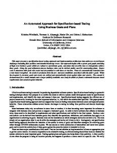
Traditionally, performance testing starts first with identifying key performance scenarios, based on the idea that certain scenarios are more frequent than others or certain scenarios impact more on the performance of the system than other scenarios. A performance scenario is a sequence of actions performed by an identified group of users (Petriu and Shen, 2002). However, this has traditionally been a manual step in the performance testing process. Typically, the identified scenarios are put together in a model or subprogram and later executed to produce load that is sent to the system. In our approach, we use probabilistic timed automata (PTA) (Jurdzi´nski et al., 2009) to model the likelyhood of user actions. The PTA consists of a set of locations interconnected to each other via a set of edges. A PTA also includes the notion of time and probabilities (see Figure 1(a)). Edges are labeled with different values: probability value, think time, and action. The probability value represents the likelihood of that particular edge being taken based on a probability mass function. The think time describes the amount of time that a user thinks or waits between two consecutive actions. An action is a request or a set of requests that the user sends to the system. Executing an action means making a probabilistic choice, waiting for the specified think time, and executing the actual action. In order to reduce complexity of the PTA, we use a compact notation where the probability value, think time, and action are modeled on the same edge (see Figure 1(b)).

4

AUTOMATIC WORKLOAD MODEL CREATION

In this section, we describe the method for automatically creating the workload model from log data and we discuss relevant aspects in more detail. The starting point of our approach is a web server log provided by web servers such as Apache or Microsoft Server. A typical format for a server log is shown in Table 1. The log is processed in several steps and a workload model is produced.

1 1.0 / 4 / action2()

0.6 / 3 / action1() 0.4 / 4 / action2()

1.0 / 0 /

6

2

7

3 1.0 / 6 / exit() 1.0 / 8 / exit()

1.0 / 6 / exit() 1.0 / 8 / exit() 8

4

(a) Original PTA (b) Compact PTA Figure 1: Example of a probabilistic timed automata

4.1

Data Cleaning

Before we start parsing the log file we prepare and clean up the data. This entails that irrelevant data is removed from the log. Nowadays, it is not uncommon to encounter requests made by autonomous machines, also referred to as bots, usually used to crawl the web and index web sites. These types of requests are identified and removed from the log into a separate list. At the moment, we are only interested in HTTP requests that result in a success or redirect (i.e., response codes that start with 2xx or 3xx). Requests that result in an error, typically response codes that start with 4xx or 5xx, are usually not part of the intended behavior and are also put in a separate list.

4.2

Parsing

The cleaned log file is parsed line by line using a pattern that matches the logging format. In our approach, a new virtual user is created when a new client IPaddress1 is encountered in the log. For each request made to the sever, the requested resource is stored in a list associated with a virtual user. The date and time information of the request together with the time difference to the previous request is also stored. The latter is what we denote as think time between two requests.

4.3

Pre-processing

From the previous step, we obtain a list of virtual users and for each virtual user a list of requests made 1 Our approach uses IP-addresses for user classification since the UserId is only available for authenticated users and usually not present in the log.

Client IP-address 87.153.57.43 87.153.57.43 87.153.57.43 136.242.54.78 136.242.54.78 136.242.54.78

User-Identifier example.site.com example.site.com example.site.com example.site.com example.site.com example.site.com

User Id bob bob bob alice alice alice

Date [20/Aug/2013:14:22:35 -0500] [20/Aug/2013:14:23:42 -0500] [20/Aug/2013:14:23:58 -0500] [21/Aug/2013:23:44:45 -0700] [21/Aug/2013:23:46:27 -0700] [21/Aug/2013:23:57:02 -0700]

Method GET GET GET GET GET GET

Resource /browse /basket/book/add /basket/book/delete /browse” /basket/phone/add /basket/view.html

Protocol HTTP/1.0 HTTP/1.0 HTTP/1.0 HTTP/1.0 HTTP/1.0 HTTP/1.0

Status Code 200 200 200 200 200 200

Size of Object 855 685 936 855 685 1772

Table 1: Requests to be structured in a tree

from the same client IP-address. In the pre-processing phase, these lists of requests are split up into shorter lists called sessions. A session is a sequence of requests made to the web server which represent the user activity in a certain time interval. It is not always trivial to say when one session ends and another begins, since the time interval varies from session to session. Traditionally, a session ends when a certain period of inactivity is detected, (e.g., 30 minutes). Hence, we define a session timeout value which is used to split the list of requests of a given user into sessions. In other words, we are searching for a time gap between two successive requests from the same virtual user that is greater than the specified timeout value. When a gap is found, the request trace is split into a new session. An example using a timeout of 30 minutes is shown in Figure 2.

Time Out Value 30 min Req1

Req2 1 min

Req3 3 min

Req4 32 min

Req5 12 min

Req6 5 min

35 min

GAP

Req1

Req2 1 min

Req3 3 min

Req7

Req8 22 min

GAP

Req4 12 min

Req5

Req6 5 min

Req7

Req8 22 min

Figure 2: Example of splitting a list of requests into shorter sessions

4.4

Building a Request Tree

Visitors interact with web sites by carrying out actions. Actions can be seen as abstract transactions or templates that fit many different requests. These requests can be quite similar in structure, yet not identical to each other. For example, consider a normal web shop where users add products to the basket. Adding two different products to the basket will result in two different web requests even though the action is the same. In this step, we group similar requests into actions. To achieve this, we first put the requests into a tree structure. For example, consider the example in Ta-

/

[Collection] [Resource]

/ /basket

/basket

action

/book

/book, phone /add 1 /delete 1

/phone

/add 2 /delete 1 /view.html 1

/add 1 /browse 2 /view.html 1 /browse 2

Figure 3: Example of request tree reduction.

ble 1. We split the string of the requested resource by the ”/” separator and structure it into a tree. Figure 3-left shows how the requests in Table 1 would be structured. We always keep count of how many times we end up in a leaf node. For each new log line, we try to fit the request into the tree, otherwise a new branch is created. After parsing a large log file, we obtain a large tree that might be difficult to manage. However, the tree can be reduced into a smaller tree by grouping together nodes. The algorithm is recursive and nodes at the same level in the tree are grouped together if they share joint sub-nodes. Figure 3-right shows how a tree can be reduced into a smaller tree. Once the request tree has been reduced as much as possible, every path in the reduced tree, that reaches a leaf node, is then considered as an action that can be executed against the system. Consider the second request made by both Bob and Alice in Table 1. These two requests are basically the same type of request. They both request a resource from the same collection. This is similar to a REST interface where one uses collections and resources. It would seem obvious that these two requests are the result of the same action, only that the user requested different resources. Hence, by grouping together requests of the same type to the same resources, the tree can be reduced to a smaller tree. Similar requests are grouped into an action. Requests in the tree can also be joined by manually inspecting the tree and grouping nodes that are a result of the same action. If a node in the path has more than one parameter, (e.g., it is a result of

grouping two resources) that part of the request can be parameterized. For example, the request ”/basket/book,phone/add” is a parameterized action where either book or phone should be used when sending the actual request to the system.

4.5

User Classification

Before we start constructing a workload model representing the user behavior, we cluster different virtual users into groups according to their behavior. By user behavior we mean a behavioral pattern that a group of web site visitors have in common. A User Type can be seen as a group abstracting several visitors of a web site. To group visitors based on the actions they perform we use the K-means algorithm (MacQueen, 1967). Table 2 shows the properties used for clustering. The properties are the actions obtained from the reduced request tree and the numbers represent the number of times a visitor has performed that action. Figure 5 show how the different visitors in Table 2 would be clustered into groups (or User Types) using the K-means algorithm. The only input in this step is the number of desired clusters which has to be specified a priori. Figure 4 depicts a typical example of clustering data into two groups using K-means. K-means clustering is an old method that involves assigning data points to k different clusters so that it minimizes the total squared distance between each point and its closest cluster center. One of the most widely used algorithms is simply referred to as ”Kmeans” and it is a well documented algorithm that have several proposed optimization to it. The clustering is executed as follows: 1. Choose k clusters and initialize the centroid by uniformly choosing a random value from the data points. 2. For every sample in the data set, assign it to the closest cluster using the Euclidean distance. 3. Calculate a new centroid for every cluster by computing the average of all samples in the cluster. 4. Repeat step 2 and 3 until the clusters no longer change. Virtual User Visitor 1 Visitor 2 Visitor 3 Visitor 4 Visitor 5 Visitor 6

Action1 2 0 1 4 0 5

Action2 0 3 0 6 0 2

Action3 0 4 1 0 4 0

Action4 3 3 8 0 8 7

Action5 3 3 9 1 7 0

Table 2: Example showing the number of actions that different visitors perform.

Figure 4: Example of two dimensional K-means clustering User Type 2 User Type 1

Visitor 3

Visitor 1 Visitor 4

Visitor 5

Visitor 6

Visitor 2

Figure 5: K-means clustering on data from Table 2.

Our approach also allows us to cluster virtual users based on other characteristics. Table 3 shows an example using different clustering parameters. Here the variable #Get means the total number of GET requests sent to the system and #Post means the total number of POST requests sent to the system. ATT stands for Average Think Time, ASL stands for Average Session Length, and ADT stands for Average Response Size. Virtual User Visitor 1 Visitor 2 Visitor 3 Visitor 4

#Get 25 17 31 19

#Post 3 0 3 1

ATT 44 25 54 23

ASL 653 277 1904 444

ARS 696 1353 473 943

Table 3: Example showing different clustering parameters.

This method, however, gives a different clustering result than the method presented previously and can be used as a complement if the first method gives an unsatisfactory result.

4.6

Removing Infrequent Sessions

Before we start building the workload model for each selected cluster, we filter out low frequency sessions. If we would include all possible sessions in the final workload model it would become too cluttered and difficult to understand and would include actions which do not contribute significantly to the load due to their low frequency rate. We are mainly interested in the common group behavior among visitors in the same cluster. Removing sessions that have low frequency is achieved by sorting the sessions in descending order according to their execution rate. We filter out

low frequent sessions according to a Pareto probability density function (Arnold, 2008) by cutting off the tail beneath a certain threshold value. The threshold value is given as a percentage value. That means that sessions below the threshold are simply ignored and treated as irrelevant. The threshold value can however be adjusted on-the-fly to include more or fewer sessions in the workload model. Table 4 shows an example of sessions listed in a descending order according to their execution count. There is a total of 20 sessions, some of them have been executed several times, (e.g., session 1 has been executed 7 times). A threshold value of 0.7 would in this case mean that we want 70 percent of the most executed sessions included in our model, meaning a total of 14 sessions. Thus, we would have to construct a model with (Session1 * 7) + (Session2 * 6) + (Session3 * 1). Session Session 1 Session 2 Session 3 Session 4 Session 5 Session 6 Total

Number of times executed 7 6 3 2 1 1 20

Table 4: Sessions listed in a descending order according to number of times executed.

4.7

Building the Workload Model

The workload models that we create describes the common behavior of all virtual users belonging to the same cluster. We say that the model describes the behavior of a particular User Type. Creating the model for a particular user type is a step-wise process where we overlap sessions of all visitors belonging to the same cluster. Session by session we gradually build a model, while reusing existing nodes in the model as much as possible. At each step, we note the number of times an edge has been traversed, the action, and the think time value. We use this information to calculate the probability and average think time of each edge in the model. Figure 6 depicts how the workload model is gradually built. One session at a time is included in the workload model. An edge represents an action being sent to the system. The numbers associated to the edges represent session IDs. Each node represents a place, where the visitor waits before sending the next action. One by one we include all the session belonging to the same cluster, while reusing existing nodes as much as possible. Identical sessions will be laid on top of each other and at each step, we note the number of times an edge has been traversed, the action, and

the think time value. We use this information to calculate the probability and average think time of each edge.

Figure 6: Model built in a step-wise manner.

We calculate the probability for an action as the ratio of a particular action to all the actions going out from a node. In a similar way, we calculate the think time of an action by computing the average of all think time values of an action. In order to guarantee that the workload generated from the workload model matches the workload present in the log file, we calculate the user arrival rate. This information together with the distribution between user types is described in a higher level model called the root model. Figure 7 depicts such a model. 1 0.1 / 45 / user_type1

0.4 / 60 / user_type2 0.5 / 20 / user_type3 2

Figure 7: Root model describing different user types their waiting times and probability

The labels on the edges are separated by a ”/” and refer to the probability, waiting time, and user type, respectively. The probability value describes the distribution between different user types. The waiting time describes the average waiting time between sessions. The user type value simply denotes what workload model to execute. To calculate the waiting time of a user type, we first have to study the waiting time between different sessions of a particular user. We then calculate the user waiting time by computing an

average time between sessions for every user belonging to a cluster.

5

TOOL SUPPORT

Tool support for our approach was implemented using the Python (Python, 2014) programming language. To increase the performance of the tool and make use of as many processor cores as possible for the most computation intensive tasks, we made use of Python’s multiprocessing library. Our tool has a set of pre-defined patterns for common logging formats that are typically used in modern web servers (e.g., Apache and Microsoft Server). However, if the pattern of the log file is not automatically recognized (e.g., due to a custom logging format) the user can manually specify a logging pattern via a regular expression. Once the log is parsed, the data is stored into a database. This way we avoid having to re-parse large log files from one experiment to another. Before parsing a log file, the tool prompts the user for a session time out value and the number of user clusters. This information, however, has to be provided a priori. Once the file has been parsed and the reduced request tree has been built, the user has a chance to manually inspect the tree. Requests can be grouped manually by dragging one node on top of the other. Figure 8 shows an example of such a request tree. When the workload models have been built for each cluster they are presented to the user. Figure 9 shows an example where 2 clusters have been used. The left pane shows the number of concurrent users detected throughout the logging period. The slider bar at the bottom of the figure can be used to adjust the threshold value, which determines how many sessions to include in the model. A higher threshold value usually means more sessions are included in the model, leading to a more complex model. When saving the model, the tool will create two artifacts: the workload models and the Python adapter code. The latter contains the mapping of each action in the models in a parameterized form and is used to interface our MBPeT tool with the system under test.

6

Example

In this section, we apply our approach to a web log file containing real-users data.

Figure 8: Example of the request tree

The web site2 used in this example maintains scores of football games played in the football league called pubiliiga. It also stores information about where and when the games are played, rules, teams, etc. The web site has been created using the Django framework (Django Framework, 2012) and runs on top of an Apache web server.

6.1

Data Cleaning

The log that we used was 323 MB in size and contained roughly 1.3 million lines of log data. The web site was visited by 20,000 unique users that resulted in 365,000 page views between April 25th of 2009 and August 23rd of 2013. However, most of the users only visited the web site once or twice and there were only about 2,000 frequent users that regularly visited the web site. Also, since the web site is updated frequently on the same platform on which it is running, the log contained a significant amount of data from erroneous requests made by the simple method of trail and error during development. All erroneous requests and requests made from known robots were filtered out. The results that we are going to show in this section are generated from a selected section of the log data containing a mere 30,000 lines of log data, gen2 www.pubiliiga.fi

Figure 9: The output window

1 0.44 / 6 / action27 0.20 / 5 / action26 4

0.097 / 0 / exit()

8

0.17 / 11 / action23

0.55 / 0 / exit()

5

0.043 / 5 / action24 0.086 / 0 / action22

0.29 / 5 / action22 1 / 22 / action22

3

0.043 / 0 / action20

6

0.16 / 23 / action22

1 / 0 / exit() 0.84 / 0 / exit()

0.032 / 22 / action25 9

1 / 4 / action20

1 / 0 / exit()

7

0.054 / 0 / action23

10

1 / 0 / exit()

1 / 0 / exit()

2

Figure 10: Workload models recreated from log data.

erated by 1092 unique users.

6.2

Pre-Processing

We used a session timeout value of 60 minutes to determine where to split the list of requests into ses-

sions. In this experiment, we clustered the users into two different groups. The total time to parse and preprocess the data was around 10 seconds. The computer was equipped with a 8 core Intel i7 2.93 GHz processor and had 16 GB of memory.

6.3

Results

We used a threshold value of 0.3 when reconstructing the workload model for both clusters, meaning that 30 percent of most executed traces are included in the models. Figure 10 shows the workload model for cluster 1. A total of 985 virtual users were grouped into this cluster. For confidentiality reasons the actual request types have been left out and replaced by abstract types. Creating the model took approximately 2 seconds. However, the execution time may hugely vary depending on the number of sessions that need to be included in the workload model. That number of sessions included in the model depends on what threshold value is selected.

7

VALIDATION

In this section, we demonstrate the validity of our approach on an auctioning web service, generically called YAAS (Yet Another Auction Site). The YAAS web service was developed as a university stand-alone project. The web service has a RESTful interface and has 5 simple actions: • Browse: Returns all active auctions. • Search: Returns auctions that matches the search query. • Get Auction: Returns information about a particular auction. • Get Bids: Returns all the bids made to a particular auction. • Bid: Allows an authenticated user to place a bid on an auction. During this experiment we preformed two load tests. First, we generated load from workload models that we built manually. We then re-created the workload models from the log data that was produced during first load test. In the second load test, load was generated from the re-created workload models. Finally, we compared the load that was generated during both tests. In the first step, we manually created models for two different user types. To test if the clustering works as expected, we made the workload models almost identical except for one request. One user type is doing distinctively a browse request while the other user type is always doing a search request. Figure 11(a) depicts the model for user type 1, the one that is performing distinctively a browse request. A similar model was also created for user type 2. If the algorithm can cluster users into different groups when only one action distinguishes them, then we consider the clustering to be good enough.

7.1

Generating a log file

Once the models were built, they were used to load test the YAAS system using our in-house performance testing tool MBPeT. We simulated 10 virtual users (60% user type 1 and 40% user type 2) in parallel for 2 hours. We set the virtual users to wait 20 seconds between each session. This value is later going to influence the timeout value during pre-processing phase. From the produced log file, containing roughly 10,000 lines, we re-created the original models as accurately as possible. We point out that the original model is of a probabilistic nature, which means that distinctly different traces with different lengths can be generated from a fairly simple model. For example, the shortest session had only 1 action, while the longest session had 22 actions. Also, we do not have exact control over how many times each trace is executed by a user.

7.2

Recreating the models

To make sure that we split the sessions in a similar way we used a timeout value of 20 seconds. No other delay between the requests was that large. We also clustered the data into 2 user types. Each user type is later going to be represented with a separate workload model. In this experiment we did not filter out any user sessions, hence we used a threshold value of 1.0, meaning all traces found in the log were used to recreate the models. Figure 11(a) shows the original workload model while Figure 11(b) shows the reconstructed workload model for User Type 1. A similar model was also created for User Type 2. As one can see, the only difference from the original model is the probability values on the edges. However close, the probability values in the original models do not match exactly those in the generated workload models. This is due to the fact that we use a stochastic model for generating the load and we do not have an exact control of what traces are generated. Figure 12(a) shows original root model while Figure 12(a) shows the re-created root model. From the figures we can see that the probability values of the re-created root model match that of the original root model (60% and 40%) and that the waiting time is close to 20 seconds (19.97 and 19.98).

7.3

Data Gathering

Even though the models look similar, we also wanted to make sure that the load generated from the original models matched the load generated from our recreated models. Hence, we let the MBPeT tool mea-

1 1

1.0 / 0 / browse() 2

1.0 / 0 / browse()

0.10 / 7 / browse()

3

0.87 / 4 / get_auction(id) 0.05 / 4 / browse() 3

0.20 / 5 / browse()

4

0.75 / 4 / get_bids(id) 0.03 / 0 / exit()

0.24 / 5 / browse()

0.25 / 6 / browse() 0.45 / 4 / get_bids(id)

4

0.23 / 6 / browse()

0.75 / 5 / get_bids(id) 0.033 / 0 / exit()

0.20 / 0 / exit() 0.50 / 3/ bid(id,price,username,password) 0.30 / 0 / exit()

0.095 / 7 / browse()

0.87 / 4 / get_auction(id) 0.052 / 4 / browse()

0.48 / 4 / get_bids(id)

5 0.20 / 0 / exit()

5

0.48 / 3 / bid(id, price, username, password)

0.29 / 0 / exit()

0.30 / 0 / exit()

6 0.30 / 0 / exit()

6

2

(a) User Type 1 original model. (b) User Type 1 recreated model. Figure 11: Original and re-created workload models.

load test 2 is virtually identical with 1.38 req/sec. Figure 13 shows the workload as a function of request (actions) over time for both test sessions. As one can see, the graphs are not identical but the trend and scale is pretty much similar.

(a) Original root model.

8

(b) Recreated root model. Figure 12: Root models

sure the number of requests sent to the YAAS system during both steps. Table 5 shows a comparison between the tests. Request Search(string) Browse() Get Auction(id) Get bids(id) Bid(id, price, username, password) Total Request Rate

Load Test 1 1263 1895 2762 2697 1288 9903 1.37 req/sec

Load Test 2 1294 1942 2821 2625 1265 9947 1.38 req/sec

Table 5: Comparison between the two test runs

As can be seen from the table, the re-created model produced a slightly higher workload. However, we like to point out that the load generation phase lasted for 2 hours and we see a difference of 44 requests. This is backed up by looking at the measured request rate. Load test 1 generated 1.37 req/sec, while

CONCLUSIONS

In this paper, we have presented a tool-supported approach for creating performance models from historical log data. The models are of a stochastic nature and specify the probabilistic distribution of actions that are executed against the system. The approach is automated, hence reducing the effort necessary to create workload models for performance testing. In contrast, Cai et al. (Cai et al., 2007) report that they spent around 18 hours to manually create a test plan and the JMeter scripts for the reference Java PetStore application (Oracle, 2014). The experiments presented in this paper have shown that the approach can adequately enough create workload models from log files and they mimic the real user behavior when used for load testing. Further, the models themselves give insight in how users behave. This information can be valuable for optimizing functions in the system and enforcing certain navigational patterns on the web site. Future work will targeted towards handling larger amount of log data. Currently the tool is not optimized enough to operate efficiently on large data amounts. Another improvement is automatic session detection. Currently the tool follows a pre-defined timeout value for detecting sessions. Automatic session detection could suggest different timeout values

(a) Load Test 1

(b) Load Test 2 Figure 13: Number of request shows as a function over time

for different users, hence, improving on the overall quality of the recreated model. Currently, we are only clustering users according to accessed resources. In the future, we would like to extend the K-means clustering algorithm to cluster based on other relevant factors like: request method, size of resource, user request rate, etc. This clustering method could suggest models that, when executed, exercise the workload patterns on the system, thus, potentially finding ”hidden” bottlenecks. Further, an interesting experiment would be to analyze only failed or dropped requests.

This way one could for instance study the details of how a DoS-attack was carried out and what pages were hit during the attack.

ACKNOWLEDGEMENTS Our sincerest gratitude go to the owners of www.pubilliiga.fi for letting us use their data in our experiments.

REFERENCES Abbors, F., Ahmad, T., Truscan, D., and Porres, I. (2012). MBPeT: A Model-Based Performance Testing Tool. 2012 Fourth International Conference on Advances in System Testing and Validation Lifecycle. Al-Jaar, R. (1991). Book review: The art of computer systems performance analysis: Techniques for experimental design, measurement, simulation, and modeling by raj jain (John Wiley & Sons). SIGMETRICS Perform. Eval. Rev., 19(2):5–11. Anastasiou, N. and Knottenbelt, W. (2013). Peppercorn: Inferring performance models from location tracking data. In QEST, Lecture Notes in Computer Science, pages 169–172. Springer. Arnold, B. (2008). Pareto and generalized pareto distributions. In Chotikapanich, D., editor, Modeling Income Distributions and Lorenz Curves, volume 5 of Economic Studies in Equality, Social Exclusion and WellBeing, pages 119–145. Springer New York. Cai, Y., Grundy, J., and Hosking, J. (2007). Synthesizing client load models for performance engineering via web crawling. In Proceedings of the Twentysecond IEEE/ACM International Conference on Automated Software Engineering, ASE ’07, pages 353– 362. ACM. Django Framework (2012). Online at https://www.djangoproject.com/. Ferrari, D. (1984). On the foundations of artificial workload design. In Proceedings of the 1984 ACM SIGMETRICS conference on Measurement and modeling of computer systems, SIGMETRICS ’84, pages 8–14, New York, NY, USA. ACM. Jurdzi´nski, M., Kwiatkowska, M., Norman, G., and Trivedi, A. (2009). Concavely-Priced Probabilistic Timed Automata. In Bravetti, M. and Zavattaro, G., editors, Proc. 20th International Conference on Concurrency Theory (CONCUR’09), volume 5710 of LNCS, pages 415–430. Springer. Kathuria, A., Jansen, B. J., Hafernik, C. T., and Spink, A. (2010). Classifying the user intent of web queries using k-means clustering. In Internet Research, number 5, pages 563–581. Emerald Group Publishing. Lutteroth, C. and Weber, G. (2008). Modeling a realistic workload for performance testing. In 12th International Conference on Enterprise Distributed Object Computing., pages 149–158. IEEE Computer Society. Ma, S. and Hellerstein, J. L. (2001). Mining partially periodic event patterns with unknown periods. In Proceedings of the 17th International Conference on Data Engineering, pages 205–214, Washington, DC, USA. IEEE Computer Society. MacQueen, J. B. (1967). Some methods for classification and analysis of multivariate observations. In Proceedings of 5-th Berkeley Symposium on Mathematical Statistics and Probability, number 1, pages 281– 297. Berkeley, University of California Press. Mannila, H., Toivonen, H., and Inkeri Verkamo, A. (1997). Discovery of frequent episodes in event sequences. Data Min. Knowl. Discov., 1(3):259–289.

Oracle (2014). Java Pet Store 2.0 reference application. http://www.oracle.com/technetwork/java/index136650.html. Last Accessed: 2014-05-23. Petriu, D. C. and Shen, H. (2002). Applying the UML Performance Profile: Graph Grammar-based Derivation of LQN Models from UML Specifications. pages 159–177. Springer-Verlag. Python (2014). Python programming language. Online at http://www.python.org/. Last Accessed: 2014-05-23. Richardson, L. and Ruby, S. (2007). Restful web services. O’Reilly, first edition. Rudolf, A. and Pirker, R. (2000). E-Business Testing: User Perceptions and Performance Issues. In Proceedings of the First Asia-Pacific Conference on Quality Software (APAQS’00), APAQS ’00, pages 315–, Washington, DC, USA. IEEE Computer Society. Shi, P. (2009). An efficient approach for clustering web access patterns from web logs. In International Journal of Advanced Science and Technology, volume 5, pages 1–14. SERSC. Subraya, B. M. and Subrahmanya, S. V. (2000). Object driven performance testing in web applications. In Proceedings of the First Asia-Pacific Conference on Quality Software (APAQS’00), pages 17–26. IEEE Computer Society. Vaarandi, R. (2003). A data clustering algorithm for mining patterns from event logs. In Proceedings of the 3rd IEEE Workshop on IP Operations and Management (IPOM03), pages 119–126. IEEE.