544
WEI ZHAO, YIMIN WEI, ET AL., AN EFFICIENT ALGORITHM BY KURTOSIS MAXIMIZATION IN REFERENCE-BASED ...
An Efficient Algorithm by Kurtosis Maximization in Reference-Based Framework Wei ZHAO, Yimin WEI∗ , Yuehong SHEN, Yufan CAO, Zhigang YUAN, Pengcheng XU, Wei JIAN College of Communications Engineering, PLA University of Science and Technology, Houbiaoying Road No.88, Qinhuai District, 210007 Nanjing, China ∗ Corresponding
author’s email:
[email protected]
Abstract. This paper deals with the optimization of kurtosis for complex-valued signals in the independent component analysis (ICA) framework, where source signals are linearly and instantaneously mixed. Inspired by the recently proposed reference-based contrast schemes, a similar contrast function is put forward, based on which a new fast fixed-point (FastICA) algorithm is proposed. The new optimization method is similar in spirit to the former classical kurtosis-based FastICA algorithm but differs in the fact that it is much more efficient than the latter in terms of computational speed, which is significantly striking with large number of samples. The performance of this new algorithm is confirmed through computer simulations.
Keywords Blind source separation, independent component analysis, kurtosis, reference-based contrast functions, fastICA, complex-valued signals
1. Introduction Independent component analysis (ICA) is a statistical method for transforming an observed multidimensional random vector into components that are statistically as independent from each other as possible [1]. In a multi-input/multioutput (MIMO) context, the problem of ICA has found interesting solutions through the optimization of so-called contrast (objective) functions [2], many of which rely on higherorder statistics (e.g., the kurtosis contrast [3], [4]) or can be linked to higher-order statistics (e.g., the constant modulus contrast function [5]). These criteria are known to provide good results. Recently, contrast functions referred to as “referencebased” have been proposed [6], [7] which are based on crossstatistics or cross-cumulants between the estimated outputs and reference signals [6]-[12]. Due to the indirect involvement of reference signals in the iterative optimization pro-
DOI: 10.13164/re.2015.0544
cess, these reference-based contrast functions have an appealing feature in common: the corresponding optimization algorithms are quadratic with respect to the searched parameters. Taking advantage of this quadratic feature, a maximization algorithm based on singular value decomposition (SVD) has been proposed [6], [7] and was shown to be significantly quicker than other maximization algorithms. However, this method generally requires an additional “fixpoint” like iteration to improve the separation quality and often suffers from the need to have a good knowledge of the filter orders due to its sensitivity on the rank estimation. A new kurtosis-based gradient algorithm with reference signals fixed has been proposed in [11], which overcomes the drawbacks of SVD based method well. Similarly, an improved algorithm with reference signals update after each one-dimensional optimization has been presented in [12], which shows better performance. Based on [11] and [12], a new family of algorithms to maximize a kurtosisbased contrast function is proposed [7], whose global convergence to a stationary point is proved. And a tradeoff can be adjusted between performance and speed of the optimization method. Inspired by [7] and [12], a similar reference-based contrast function is constructed, based on which a novel algorithm is proposed for complex-valued signals. More precisely, the cross-cumulant between estimated signals and reference signals is utilized as the contrast criterion in terms of kurtosis. Due to the quadratic dependence on the searched parameter, the main advantage of our proposed algorithm consists in the fact that it is much more efficient than the classical one in terms of computational speed. The performance of our method is validated through computer simulations. Note that the work of this paper is the extension of that in [13] that only considers the real-valued signals. The remaining of this paper is organized as follows. Section 2 introduces the system model and assumptions. The contrast criteria including reference signals and corresponding contrast functions are presented in Section 3. Our new proposed optimization algorithm is shown in Section 4. Computer simulations are performed in Section 5. Section 6 concludes this paper.
SIGNALS
RADIOENGINEERING, VOL. 24, NO. 2, JUNE 2015
545
2. System Model and Assumptions 2.1 System Model In this paper, we extend our work in [13] to the complex-valued signal separation model. The system model for ICA is shown in Fig. 1, in which the mixing system is noise-free.
x1(t)
s1 (t ) s2 (t )
sN1 (t )
xN2 (t )
A
W
y N1 (t )
Fig. 1. System model.
Sources are denoted by s(t) = [s1 (t), · · · , sN1 (t)]T = [s1r (t) + is1i (t), · · · , sN1 r (t) + isN1 i (t)]T . The observed (mixed) signals are denoted by x(t) = [x1 (t), · · · , xN2 (t)]T = [x1r (t) + ix1i (t), · · · , xN2 r (t) + ixN2 i (t)]T . The input-output relationship can be described as x (t) = As (t)
(1)
where A is the mixture matrix of N2 × N1 , representing the linear mixing system, which is composed of N2 row complex-valued vectors, i.e., A = [a1 , a2 , · · · , aN2 ]T . The separated signals are denoted by y (t) = [y1 (t) , · · · , yN1 (t)]T = [y1r (t) + iy1i (t), · · · , yN1r (t) + iyN1 i (t)]T , which results from H
y (t) = W x (t)
2.3 Assumptions In order to retrieve the sources blindly and successfully, we make two assumptions [7], which are shown as follows:
y1(t) y2 (t)
x2 (t)
the spectrum efficiency and computational speed of wireless communication system. The corresponding work will be investigated and shown in our latter work. We believe this kind of wireless communication system is very significant and promising in the future.
(2)
where W is the separation matrix of N2 × N1 , representing the linear separating system, which contains N1 column complex-valued vectors, i.e., W = [w1 , w2 , · · · , wN1 ]. WH stands for the Hermitian of W, that is W is transposed and conjugated. Without loss of generality, we assume the number of sources equal to that of observed signals, i.e., N1 = N2 = N in this paper.
2.2 Practical Model For practical application of our algorithm for the complex-valued signals, we are planing to construct a wireless communication system with two transmitting and receiving antennas, which transmits multiple signals simultaneously in the same frequency band over wireless channel and recovers the source signals at the multiple-antenna receiver by utilizing the statistical characteristics of source signals and broadcasting characteristics of wireless channel. Therefore, the spectrum efficiency of this system is high compared to that of time division multiplexing (TDM), frequency division multiplexing (FDM), and code division multiplexing (CDM). If it works, our new algorithm can improve
A1. The sources processes si (t), statistically mutually independent.
i ∈ {1, · · · , N} are
A2. All the components of s (t) are stationary, zeromean and they have unit variances and uncorrelated real and imaginary parts of equal variances, i.e., E{s (t) s(t)H } = I and E{s (t) s(t)T } = 0.
3. Contrast Criteria 3.1 Reference Signals Before introducing the contrast function, we first give a brief introduction of the reference signals referred to above. As shown in [6]-[12], the reference signals are expressed in the form of z (t) = VH x (t)
(3)
where z(t) and V are set similarly as y (t) = WH x (t), which are denoted by z (t) = [z1 (t) , · · · , zN (t)]T = [z1r (t) + iz1i (t), · · · , zN1r (t) + izNi (t)]T and V = [v1 , v2 , · · · , vN ], respectively. However, the reference signals are artificially introduced in an algorithm for the purpose of facilitating the maximization of the contrast function [6], [7]. In [11], the reference signals are initialized arbitrarily and kept the same during the whole optimization process. In [12], the reference signals are not directly involved in the iterative optimization computation. In other words, the reference signals update following the objective signals. More precisely, V updates following W in each loop iteration step. Then the separation quality of the algorithm in [10] is better than that in [11]. In [14] and [15], we have done some corresponding work to investigate the impact of reference signals, which is similar to [12]. Combined with [12], we only consider the case where the reference signals are successively updated after each one-dimensional optimization. In [13], we have done some similar work on real-valued signals, which is extended to the complex-valued signals in this paper. Therefore, the performance of our algorithms is much better than those in [14] and [15]. Since no confusion is possible and for simplicity, in the following sections, we drop the time index and these vectors are denoted respectively by s, x, y and z.
546
WEI ZHAO, YIMIN WEI, ET AL., AN EFFICIENT ALGORITHM BY KURTOSIS MAXIMIZATION IN REFERENCE-BASED ...
3.2 Contrast Functions In order to describe the contrast function used in this paper, we first introduce some notations. The cumulant of a set of random variables is denoted by Cum{•}. We consider the cumulant of complex-valued signals [7]. For any jointly stationary signals y(t) and z(t), with zero-mean, we set C{y} = Cum {y(t), y(t)∗ , y(t), y(t)∗ } = E{y(t)y(t)∗ y(t)y(t)∗ } − E{y(t)y(t)∗ }E{y(t)y(t)∗ } − E{y(t)y(t)}E{y(t)∗ y(t)∗ } − E{y(t)y(t)∗ }E{y(t)∗ y(t)} = E{|y(t)|4 } − 2(E{|y(t)|2 })2 − E{(y(t))2 }E{(y(t)∗ )2 }, (4) Cz {y} = Cum {y(t), y(t)∗ , z(t), z(t)∗ } = E{y(t)y(t)∗ z(t)z(t)∗ } − E{y(t)y(t)∗ }E{z(t)z(t)∗ } − E{y(t)z(t)}E{y(t)∗ z(t)∗ } − E{y(t)z(t)∗ }E{y(t)∗ z(t)} = E{|y(t)|2 |z(t)|2 } − 2E{|y(t)|2 }E{|z(t)|2 } − E{y(t)z(t)}E{y(t)∗ z(t)∗ } (5) where E{•} denotes the mean value and y∗ designates the complex conjugate of y. Let us introduce the following criteria: J(w) = C{wH x}, I(w, v) = Cz {wH x} z=vH x
(6) (7)
where J is the well-known kurtosis contrast function, which has been proved to be a contrast function [3], [4]. I is our reference-based contrast function, which is similar to those proposed in [7] and [12]. The consistent convergency of our reference-based contrast function can be proved by referring to the Proposition 1 in [7]. Recently, we also have done some corresponding work by introducing the reference signals to the negentropy contrast function, based on which a class of more efficient and robust algorithms has been proposed. These work will be presented in our latter work.
4. Optimization Algorithm Based on the assumptions and the Proposition 1 in [7], it can be concluded that the new contrast function I we propose has local extrema, which means that the stationary points of it can be found through optimization schemes. In this section, we give the derivation of our proposed algorithm in detail for the extraction of one source component. After whitening, the mixing signals x satisfies E{xxH } = I. According to the assumptions A1 and A2, E{xxT } = 0 follows straightforward from E{ssT } = 0. Un 2 der the constraint E{ wH x } = kwk2 = 1 and with v update following w, we can get I(w, v) = Cz {wH x} z=vH s H 2 H 2 2 2 = E{ w x w x } − 2E{ wH x }E{ vH x } (8) − E{(wH x)(vH x)}E{(wH x)∗ (vH x)∗ } H 2 H 2 2 = E{ w x v x } − 2 kwk2 E{ vH x }.
According to the Lagrange conditions, we construct 2 Lagrange function under the constraint E{ wH x } = kwk2 = 1: 2 L(w, λ) = I(w, v) + β(E{ wH x } − 1) H 2 H 2 2 = E{ w x v x } − 2 kwk2 E{ vH x } + β(kwk − 1). (9) Then the extrema of I(w, v) with respect to w are obtained at points where ∂L ∂w
T
2
x) } = ∇1 I(w, v) + β ∂E{(w H 2 H ∂w 2 2 = ∇1 E{ w x v x } − 4wE{ vH x } + 2βw = 0 (10)
where β ∈ R. Similar to the complex gradient in [16], we have H 2 w x = (wH x)(wH x)∗ (11) = (w1r x1r + w1i x1i + · · · + wNr xNr + wNi xNi )2 + (w1r x1i − w1i x1r + · · · + wNr xNi − wNi xNr )2 where w = [w1r , w1i , · · · , wNr , wNi ], and we assume the following notations ∆1 = w1r x1r + w1i x1i + · · · + wNr xNr + wNi xNi , (12) ∆2 = w1r x1i − w1i x1r + · · · + wNr xNi − wNi xNr . Then the first term in (10) can be expressed as 2 E{(∆1 x1r + ∆2 x1i ) vH x } 2 E{(∆1 x1i − ∆2 x1r ) vH x } .. ∇1 I(w, v) = 2 . H 2 E{(∆1 xNr + ∆2 xNi ) v x } 2 E{(∆1 xNi − ∆2 xNr ) vH x } 2 E{Re{x1 (wH x)∗ } vH x } 2 E{Im{x1 (wH x)∗ } vH x } .. . = 2 . 2 E{Re{xN (wH x)∗ } vH x } 2 E{Im{xN (wH x)∗ } vH x }
(13)
and we use Newton method to solve (9). Similar to (13), the Jacobian matrix of I(w, v), with respect to w, can be expressed as ∇21 I(w, v) = 2 + x2 ) (x1r · · · (xNi x1r − xNr x1i ) 1i (x1r x1i − x1i x1r ) · · · (xNi x1i + xNr x1r ) H 2 . . . .. .. .. 2E v x (x x + x x ) · · · (x x − x x ) Nr Ni Ni Nr Nr Ni 1r 1i 2 + x2 ) (x1r xNi − x1i xNr ) · · · (xNi Nr 2 2 (x1r + x1i ) 0 ··· 0 2 + x2 ) · · · 0 (x 0 1i 1r ≈ 4E .. .. . .. . . 0 2 + x2 ) 0 0 · · · (xNi Nr H 2 = 4I = 4E{ v x }I
(14) where the approximation was done by separating the expectations. Also, E{xxH } = I and E{xxT } = 0 are used
RADIOENGINEERING, VOL. 24, NO. 2, JUNE 2015
547
here. HAnd 2 the last2term in (14) results from the constraint E{ w x } = kwk = 1 in which v updates following w so 2 that we have E{ vH x } = kvk2 = 1. Then the total approximative Jacobian of (10) is now 2 2 J = (4E{ vH x } − 4E{ vH x } + 2β)I = 2βI
(15)
which is diagonal and thus easy to invert. We obtain the following approximative Newton iteration: 2
w0 = w − w0 =
5. Simulation Results and Analysis 5.1 Separability of Our Algorithm In this section, the separability of our proposed algorithm is investigated through simulations. Here we choose three independent 16QAM signals as sources, for which the samples T = 10000 and the iteration parameter kmax = 1000. The source signals are shown in Fig. 2.
2
2E{x(wH x)∗ |vH x| }−4wE{|vH x| }+2βw 2β
(16)
w0 kw0 k .
If we multiply both sides of (16) by 2β, then (16) can be simplified to 2 2 w0 = E{x(wH x)∗ vH x } − 2E{ vH x }w (17) w0 w0 = kw 0k . Finally, the derivation of our proposed algorithm is completed, which is summarized as follows:
Step1. Eliminate the mean value of x and prewhiten it. Step2. Initialize W, and normalize it. Step3. For i = 1, 2," , N repeat Step3 a. Set w i0 = w i , v i0 = w i0 b. For k = 0,1," , kmax − 1 repeat b 2
Set
w ik +1 = E{x((w ik ) H x)∗ ( v ik ) H x } 2
− 2 E{ ( v ik ) H x }w ik
Normalize w ik +1
w ik +1 = w ik +1 − ∑ j =1 w j w j H w i
Renormalize w ik +1
Set v ik +1 = w ik +1
w i = w ikmax −1
i −1
Step4. y = W H x
In the algorithm above, wik+1 corresponds to the ith source to be retrieved for the (k+1)th iteration step and vik+1 is the corresponding reference vector, which updates following wik+1 . From the whole process, we can see the source signals are restored one by one through each one-dimensional optimization in a deflationary manner. To prevent different one-dimensional optimization converging to the same maxima, a Gram-Schmidt-like decorrelation scheme [3], [4], [16] is adopted.
Fig. 2. Three source signals.
The observation signals are mixed through linear matrix, which is chosen arbitrarily, i.e.,
0.4261 − 0.3166i A = −1.0562 − 0.4387i −1.1510 + 0.9457i
−0.0469 + 1.5955i 1.7749 − 0.7757i 0.0562 + 0.2929i
−1.8124 − 2.0990i −0.5268 + 0.4839i 2.4162 − 0.5969i
(18) and the mixing signals are shown in Fig. 3.
548
WEI ZHAO, YIMIN WEI, ET AL., AN EFFICIENT ALGORITHM BY KURTOSIS MAXIMIZATION IN REFERENCE-BASED ...
Fig. 3. Three mixture signals.
Fig. 4. Three separation signals.
By using our algorithm introduced above, the recovered signals are shown in Fig. 4. To verify the separability of our algorithm more precisely, the separation-mixture matrix is presented as H W QA = 0.2048 − 0.5972i 0.0048 − 0.0036i −0.0026 + 0.0004i
and scaling ambiguities. However, it is fortunate that the ambiguities are common and insignificant in most applications.
5.2 Performance Analysis −0.0059 − 0.0025i 0.0011 + 0.0023i 0.4633 + 0.4250i
−0.0013 + 0.0017i −0.5823 + 0.2538i −0.0007 − 0.0041i
(19) y = WH x = WH QA =
where Q is the whitening matrix, i.e., WH QAs. Note that the element labelled in black corresponds to one of sources.
It can be observed clearly that, compared Fig. 2 and Fig. 4, our proposed algorithm recovers the source signals successfully up to some ambiguities, i.e., permutation
In this section, we choose three QAM signals as sources to investigate the performance of our proposed algorithm. The number of samples T varies from 1000 to 10000 and we set the iteration parameter kmax = 1000. The mean value of mean square error (MSE) and median MSE between sources and corresponding estimations are chosen as the performance measure criterion of separation quality. The average execution time is chosen as the measure criterion of computational speed, for which the computer is Intel(R) Core 2 Duo CPU, E8400 @ 3.0 GHz, 2.99 GHz,
RADIOENGINEERING, VOL. 24, NO. 2, JUNE 2015
549
3.00 GB RAM. In order to make the simulation results more reliable and reasonable, we perform 100 independent execution runs for each simulation, in which the mixing matrix is randomly chosen.
It can be observed clearly from Fig. 5 and Fig. 6, that the value of MSE and median MSE of our proposed algorithm F4 is very close to those of F1, F2 and F3, which means that our new method converges to the approximately identically stationary points as others. More precisely, our new algorithm recovers sources successfully on one hand, and shows similar performance in terms of separation quality on the other hand. Moreover, with the number of samples increasing, the performance of F1, F2, F3 and F4 is so close that there is no difference among them. Additionally, compared Fig. 5 and Fig. 6, we can see that our proposed method is very stable. However, in Fig. 7, it can be clearly observed that the execution time of F4 is much less than that of F1, F2 and F3, which means that our new algorithm is more efficient than others in terms of computational speed. And the advantage of our method is particularly more apparent over others with the number of samples increasing. Furthermore, the reference-based algorithms F2 and F4 show quicker convergent speed than F1 and F3, respectively. Note that we mainly focus on the fact that our new proposed FastICA algorithm F4 provides better performance than the classical one F3, which is the initial motivation of this paper.
5.3 Complexity Analysis In this section, the computational complexity of our new algorithm F4 and corresponding classical one F3 is briefly analyzed, which reveals the reason why the former is much more efficient than the latter in terms of computational speed. The main difference between F3 and F4 is 2 2 wik+1 = E{x((wik )H x)∗ (wik )H x } − 2E{ (wik )H x }wik 2 (20) 2 wik+1 = E{x((wik )H x)∗ (vik )H x } − 2E{ (vik )H x }wik (21) where (20) denotes the classical algorithm F3 and (21) denotes our proposed one F4.
F2: Gradient maximization algorithm with reference signals F3: Classical FastICA algorithm without reference signals
Average MSE
5
F4: Our proposed FastICA algorithm with reference signals
x 10
4
-6
7.3 3
7.2
2
7.1 7
1
4990 4995 5000 5005
0
2000
4000 6000 Number of samples
8000
Fig. 5. MSE between sources and corresponding estimations averaged over 100 independent runs.
6
x 10
-4 F1: Gradient maximization algorithm without reference signals F2: Gradient maximization algorithm with reference signals F3: Classical FastICA algorithm without reference signals
5 Average median MSE
Note that all the algorithms are implemented on our computer under same condition. The simulation results are illustrated in Fig. 5, Fig. 6 and Fig. 7.
-4 F1:Gradient maximization algorithm without reference signals
F4: Our proposed FastICA algorithm with reference signals
x 10
4
-6
7.4 3
7.2
2
7
1
4970 4980 4990 5000
0
2000
4000 6000 Number of samples
8000
Fig. 6. Median MSE between sources and corresponding estimations averaged over 100 independent runs.
50 F1: Gradient maximization algorithm without reference signals
Average execution time (s)
In this paper, we consider the performance comparison and analysis among four algorithms, which are denoted by F1, F2, F3 and F4. F1 denotes the gradient maximization algorithm based on kurtosis, which is similar to the optimization schemes in [6]-[12] but differs in the fact that reference signals are not considered. F2 denotes the optimization algorithm proposed in [7] and [12]. F3 denotes the classical FastICA algorithm based on kurtosis shown in [3], [4], [16]. F4 denotes our proposed FastICA algorithm with reference signals introduced.
6
x 10
F2: Gradient maximization algorithm with reference signals
40
F3: Classical FastICA algorithm without reference signals F4: Our proposed FastICA algorithm with reference signals
30
20
10
0
0
2000
4000 6000 8000 Number of samples
10000
Fig. 7. Average execution time of recovering all the sources averaged over 100 independent runs.
550
WEI ZHAO, YIMIN WEI, ET AL., AN EFFICIENT ALGORITHM BY KURTOSIS MAXIMIZATION IN REFERENCE-BASED ...
It is well accepted that the value of kurtosis has to be estimated from a measured sample in practice. So from (20) and (21), we can see that the computational complexity of F3 and F4 is thus an increasing function of the number of sources, sample size T and iterative parameter kmax . More precisely, the computational complexity mainly lies in (wik )H x, for which w updates after each iteration. However, the reference signal vector v introduced in our algorithm updates following w, which means that (vik )H x is known advance to a certain extent and is not involved in the iteration optimization process. Therefore, the computational complexity of (21) for our algorithm only relates to w and the computational resource is reduced significantly compared with (20) of the classical one, which is significantly striking with the number of samples increasing.
6. Conclusion In this paper, a new algorithm is proposed, which is based on our proposed reference-based contrast function. It is similar to the classical FastICA algorithm but is much more efficient than the latter in terms of computational speed. Computer simulations are performed to validate the performance of our algorithm. Our future work includes the extension of this new algorithm to more complex mixing models such as convolution and nonlinear, in which the noise will be considered.
Acknowledgments This work is supported by the NSF of Jiangsu Province of China under Grant No. 2012057, and by the National Natural Science Foundation of China under Grant Nos. 61172061 and 61201242.
References [1] LAHAT, D., CARDOSO, J. F., MESSER, H. Second-order multidimensional ICA: Performance analysis. IEEE Transactions on Signal Processing, 2012, vol. 60, no. 9, p. 4598–4610. DOI: 10.1109/TSP.2012.2199985 [2] COMON, P., JUTTEN, C. (Eds.) Handbook of Blind Source Separation, Independent Component Analysis and Applications. New York: Academic Press, 2010. [3] SIMON, C., LOUBATON, P., JUTTEN, C. Separation of a class of convolutive mixtures: A contrast function approach. Signal Processing, 2001, vol. 81, no. 4, p. 883–887. DOI: 10.1016/S01651684(00)00240-1 [4] TUGNAIT, J. K. Identification and deconvolution of multichannel linear non-Gaussian processes using higher order statistics and inverse filter criteria. IEEE Transactions on Signal Processing, 1997, vol. 45, no. 3, p. 658–672. DOI: 10.1109/78.558482 [5] GODARD, D. Self-recovering equalization and carrier tracking in two-dimensional data communication systems. IEEE Transactions
on Communication, 1980, vol. 28, no. 11, p. 1867–1875. DOI: 10.1109/TCOM.1980.1094608 [6] CASTELLA, M., RHIOUI, S., MOREAU, E., PESQUET, J. Quadratic higher-order criteria for iterative blind separation of a MIMO convolutive mixture of sources. IEEE Transactions on Signal Processing, 2007, vol. 55, no. 1, p. 218–232. DOI: 10.1109/TSP.2006.882113 [7] CASTELLA, M., MOREAU, E. New kurtosis optimization schemes for MISO equalization, IEEE Transactions on Signal Processing, 2012, vol. 60, no. 3, p. 1319–1330. DOI: 10.1109/TSP.2011.2177828 [8] ADIB, A., MOREAU, E., ABOUTAJDINE, D. Source separation contrasts using a reference signal. IEEE Signal Processing Letters, 2004, vol. 11, no. 3, p. 312–315. DOI: 10.1109/LSP.2003.822894 [9] CASTELLA, M., RHIOUI, S., MOREAU, E., PESQUET, J. Source separation by quadratic contrast functions: A blind approach based on any higherorder statistics. In Proceedings of IEEE International Conference on Acoustics, Speech and Signal Processing (ICASSP). Philadelphia (USA), 2005, vol. 3, p. 569–572. DOI: 10.1109/ICASSP.2005.1415773 [10] KAWAMOTO, M., KOHNO, K., INOUYE, Y. Eigenvector algorithms incorporated with reference systems for solving blind deconvolution of MIMO-IIR linear systems. IEEE Signal Processing Letters, 2007, vol. 14, no. 12, p. 996–999. DOI: 10.1109/LSP.2007.906225 [11] CASTELLA, M., MOREAU, E. A new optimization method for reference-based quadratic contrast functions in a deflation scenario. In Proceedings of IEEE International Conference on Acoust., Speech Signal Processing. Taipei (Taiwan) 2009, p. 3161 - 3164. [12] CASTELLA, M., MOREAU, E. A new method for kurtosis maximization and source separation. In Proceedings of IEEE International Conference on Acoustics, Speech and Signal Processing (ICASSP). Dallas (TX, USA), 2010, p. 2670–2673. DOI: 10.1109/ICASSP.2010.5496250 [13] ZHAO, W., WEI, Y. M., SHEN, Y. H., YUAN, Z. G., XU, P. C., JIAN, W. A novel FastICA method for the reference-based contrast functions. Radioengineering, 2014, vol. 23, no. 4, p. 1221–1225. [14] ZHAO, W., SHEN, Y. H., WANG, J. G., YUAN, Z. G., JIAN, W. New methods for the efficient optimization of cumulant-based contrast functions. In Proceedings of the 5th IET International Conference on Wireless, Mobile and Multimedia Networks. Beijing (China), 2013, p. 345–349. DOI: 10.1049/cp.2013.2438 [15] ZHAO, W., SHEN, Y. H., WANG, J. G., YUAN, Z. G., JIAN, W. New kurtosis optimization algorithms for independent component analysis. In Proceedings of the 4th IEEE International Conference on Information Science and Technology. Shenzhen (China), 2014, p. 23–28. DOI: 10.1109/ICIST.2014.6920323 [16] BINGHAM, E., HYVARINEN, A. A fast fixed-point algorithm for independent component analysis of complex valued signals. International Journal of Neural Systems, 2000, vol. 10, no. 1, p. 1–8. DOI: 10.1142/S0129065700000028
About the Authors . . . Wei ZHAO was born in 1988 in China. He is beginning to pursue the PhD degree just now. His research interests include blind source separation, independent component analysis, compressed sensing, sparse component analysis, and their corresponding applications in wireless communication systems.
RADIOENGINEERING, VOL. 24, NO. 2, JUNE 2015
Yimin WEI was born in 1973 in China. He received the PhD degree in 2012 and is now an assistant professor in PLA University of Science and Technology. His research interests include wireless communication and signal processing. Yuehong SHEN was born in 1959 in China. He received the PhD degree in 1999 and is now a professor in PLA University of Science and Technology. His research interests include wireless MIMO communication, digital signal processing, statistical signal analysis, wireless statistic division multiplexing. Yufan CAO was born in 1991 in China. He is now pursuing the Master degree in PLA University of Science and Technology. His research interests include blind source separation, independent component analysis, and their corresponding applications in wireless communication systems.
551
Zhigang YUAN was born in 1980 in China. He received the PhD degree in 2008 and is now a lecturer in PLA University of Science and Technology. His research interests include digital transmission technology and digital communication signal processing. Pengcheng XU was born in 1987 in China. He is now pursuing the PhD degree in PLA University of Science and Technology. His research interests include blind source separation, independent component analysis, and their corresponding applications in wireless communication systems. Wei JIAN was born in 1976 in China. He received the PhD degree in 2006 and is now a lecturer in PLA University of Science and Technology. His research interests include digital transmission technology and wireless communication signal processing.