An Efficient and Flexible Parallel FFT Implementation ... - TU Chemnitz
Recommend Documents
The sequences that make up the genes .... These 6-foot long strands of DNA are compacted into ... A small strand of the DNA ladder, made up of 146 base- pairs ...
Rudolph or Friedrich Försterling, Institut für Psychologie, Ludwig- ...... people; B. Paul is the kind of person that people like; C. Some other reason.â (p. 240).
Georg Nestmann. Ergänzungskurs Elementarmathematik für Bachelor WS2013/
2014. Klausurvorbereitung Teil II. Matrizen und Gleichungssysteme. 1. An 100 ...
models is that our test subjects use separate workstations ..... folder to his private folder and then load it using the ... To test the tool, constructive interaction was.
Figure 1: The clinching of sheet steels. Interesting parameters are strain and stress inside the two materials under different distri- butions of clinches. In figure 2 ...
scribe in Section 5.1 how to find optimal parameterized reduced-order models for a special case ..... Define f(s, p) = A(s, p)â1B(p)b and gT (s, p) = cT C(p)A(s, p)â1. ... So, we may calculate a directional derivative and evaluate at s = Ï and p
Introduction 0. Neurocognition. Introduction 1. Dayan, P. & Abbott, L.,. Theoretical
Neuroscience,. MIT Press, 2001. Literature. Hyvärinen, A., Karhunen, J., &.
SAP-Sicht. Die zentralen Objekte der Finanzbuchhaltung bilden Konten, zu
welchen jeweils Stammdatensätze hinterlegt werden müssen. Erst dann können.
Form von Wassertröpfchen o. a.) oder Eis vorhanden. 1.1.1 Luftzustände im h,x-
Diagramm. Für die Berechnung im Programm wurde festgelegt: • t ≥ 0,01 °C: ...
ditions is challenging due to the lack of Fréchet differentiability of the ... results for optimal control problems governed by variational inequalities other than.
Driving (EAGD) system for real time optimization and reduction of CO2 emission and ... (EAGD) with the aim to optimize t
Fluoride (AlF3) layer involved can be implemented as final process in solar cell .... a Fluorine (F) deficiency is accomplished at the in- terface AlF3|| SiO2 [3, 4, 5).
The tutorial con- cludes by giving a prototype for cluster middleware based on CORBA for heterogeneous clu- ster. ... System monitoring for ... A paper titled, "Accounting System for Linux based Network of Workstation", has been accepted for ...
wageâgood produced in a certain period, pB its price, vB the labour value incorporated ... surplus value (H-6b) or a 'temporal' rate of exploitation (H-6c) â is ...
In signal processing, it is primarily used to convert an input signal in time domain into frequency domain and vice-versa. In the world of digital, signals are ...
Mar 18, 2007 - BERND HOFMANN, PETER MATHÉ, AND SERGEI V. PEREVERZEV. Abstract. The authors study ...... [13] S. George. Newton-Lavrentiev ...
This tutorial surveys the fast Fourier transform at nonequispaced nodes (NFFT), its gener- .... A closely related matrix vector product is the adjoint NDFT h. = A.
is twofold â to shed some light on the mathematical background, as well as to provide an overview over the ..... These methods do not yield a different asymptotic.
Oct 15, 1999 - Temperature dependence of exciton peak energies in ZnS, ZnSe, ... have many potential applications in short-wavelength light- ... composed of various zinc and cadmium chalcogenides. ... meV.1â5,19â22 More recent data for Eg 300 K r
For texture one of the best ('MTEX is pretty good for texture' B.B. again) ... do things not possible in other commercial packages .... DIC Software Packages.
This program is free software: you can redistribute it. # and/or modify it under the terms of the GNU General Public. #. License as published by the Free Software ...
production lead to incommensurabilities of skills, of trajectories in the timeline that aroused by technologies at hand, ...... Bern: Haupt. Wernerfelt, B. 1984: A ...
contour into multiple segments and their treatment as open snakes allows us to exclude those parts of ... model (Cohen, 1991) a snake is able to counteract the.
27.05.2009. 1 methodenlehre ll – Grenzen des Signifikanztests. • Möglichkeiten
und Grenzen des Signifikanztests. Thomas Schäfer | SS 2009. 1 methodenlehre
...
An Efficient and Flexible Parallel FFT Implementation ... - TU Chemnitz
distributed parallel FFT agorithm and an example of its scalability limitation. P ... ability bottleneck and a software library [3] for power of two FFTs customized to.
An Efficient and Flexible Parallel FFT Implementation Based on FFTW Michael Pippig
Abstract In this paper we describe a new open source software library called PFFT [12], which was developed for calculating parallel complex to complex FFTs on massively parallel architectures. It combines the flexible user interface and hardware adaptiveness of FFTW [7] with a highly scalable two-dimensional data decomposition. We use a transpose FFT algorithm that consist of one-dimensional FFTs and global data transpositions. For the implementation we utilize the FFTW software library. Therefore we are able to generalize our algorithm straight forward to d-dimensional FFTs, d ≥ 3, real to complex FFTs, and even completely in place transformations. Further retained FFTW features like the selection of planning effort via flags and a separate communicator handle distinguish PFFT from other public available parallel FFT implementations. Automatic ghost cell creation and support of oversampled FFTs complete the outstanding flexibility of PFFT. Our runtime tests up to 262144 cores of the BlueGene/P supercomputer prove PFFT to be as fast as the well known P3DFFT [11] software package, while the flexibility of FFTW is still preserved.
1 Introduction The fast Fourier transform (FFT) provides the basis of many algorithms in scientific computing. Hence, a highly scalable implementation for massively parallel systems such as BlueGene/P is desirable. There are two approaches to parallelize multi-dimensional FFTs, first binary exchange algorithms, and second transpose algorithms. An introduction and theoretical comparison can be found in [9]. We concentrate on transpose algorithms, i.e., we perform a sequence of local FFTs and
Michael Pippig Chemnitz University of Technology, Department of Mathematics, 09107 Chemnitz, Germany, email: [email protected]
1
2
Michael Pippig
global data transpositions. For convenience, we consider a three-dimensional input dataset of size n0 × n1 × n2 with n0 ≥ n1 ≥ n2 . First parallel transpose FFT algorithms were based on a technique called slab decomposition, i.e., the three-dimensional dataset is partitioned along n0 to distribute it on a given number P ≤ n0 of MPI processes. After calculation of the n0 locally available two-dimensional FFTs of size n1 × n2 a data transposition is performed that corresponds to a call of MPI Alltoall and repartitions the three-dimensional dataset along n1 . Finally, n1 n2 one-dimensional FFTs of size n0 are computed. For example, implementations of this algorithm are included in the IBM PESSL library [5], the Intel Math Kernel Library [10], and the FFTW [7] software package, which is appreciated for its portable high-performance FFT implementations and flexible user interface. Unfortunately, all of these FFT libraries lack high scalability on massively parallel systems because slab decomposition limits the number of efficiently usable MPI processes by n1 . Figure 1 shows an illustration of the one-dimensional distributed parallel FFT agorithm and an example of its scalability limitation. n0
n2
n0
n1 T
n1
P n2
P Fig. 1 Distribution of a three-dimensional dataset of size n0 × n1 × n2 = 8 × 4 × 4 on a onedimensional process grid of size P = 8. After the transposition (T) half of the processes remain idle
A volumetric domain decomposition was used in [4, 2, 1] to overcome the scalability bottleneck and a software library [3] for power of two FFTs customized to BlueGene/L systems was implemented. The dataset is partitioned along two dimensions and therefore the number of MPI processes can be increased to at most n1 n2 . Figure 2 shows an illustration of the two-dimensional distributed parallel FFT algorithm and its improved scalability in comparison to the example in Fig. 1. Portable implementations based on two-dimensional data decomposition are the FFT package from Sandia National Laboratories [13], and the three-dimensional FFT library called P3DFFT [11]. While the FFT algorithm from Sandia National Laboratories is less restrictive on data distributions, runtime tests proved P3DFFT to perform better in most cases. It naturally turns up to ask for a public available parallel FFT library that unifies the flexibility of FFTW and the highly scalable two-dimensional data decomposition. This paper is divided into the following parts. First we give the necessary definitions and assumptions, which will endure through the whole paper. Next we show
An Efficient and Flexible Parallel FFT Implementation Based on FFTW P0
n0
n2
n1
P1 n1 n0
P1 T
n2
3
T
P0
n0
P0
n1 n2
P1
Fig. 2 Distribution of a three-dimensional dataset of size n0 × n1 × n2 = 8 × 4 × 4 on a twodimensional process grid of size P0 × P1 = 4 × 2. None of the processes remains idle in any calculation step
the key ideas to implement a parallel FFT algorithm totally based on the FFTW software library. Since P3DFFT is a well known and public available software package for parallel FFTs, we compare features of P3DFFT and our new PFFT package in Sect. 4 and their runtimes in Sect. 5. Finally, we summarize the most important results in Sect. 6.
2 Definitions and Assumptions Consider a three-dimensional dataset of n0 × n1 × n2 complex numbers gk0 k1 k2 ∈ C, ks = 0, . . . , ns − 1 for all s = 0, 1, 2. We write the three-dimensional forward discrete Fourier transform (DFT) as gˆl0 l1 l2 :=
where ls = 0, . . . , ns − 1 for all s = 0, 1, 2. It is well known that a multi-dimensional DFT can be calculated efficiently by successive one-dimensional fast Fourier transforms (FFTs). We assume further the dataset to be mapped onto a two-dimensional process grid of size P0 × P1 such that every processor owns a block of n0 /P0 × n1 /P1 × n2 complex numbers. For convenience, we claim ns to be divisible by Pr for all s = 0, 1, 2 and r = 0, 1. In order to make the following algorithms more flexible, we can easily overcome these requirements. Depending on the context we interpret the notation ns /Pr either as a simple division or as a partitioning of the dataset along dimension ns on Pr processes in equal blocks of size ns /Pr , for all s = 0, 1, 2 and r = 0, 1. This notation allows us to compactly represent the main characteristics of data distribution, namely the transposition and the partitioning of the dataset, with diagrams. For example, we interpret the notation n2 /P1 × n0 /P0 × n1 , as transposed dataset of size n0 × n1 × n2 that is distributed on P0 processes along the first dimension and on P1
4
Michael Pippig
processes along the last dimension. We assume such multi-dimensional datasets to be stored in C typical row major order, i.e., the last dimension lies consecutively in memory. Therefore, partitioning a multi-dimensional dataset can be done most efficiently along the first dimension.
3 The Parallel Three-Dimensional FFT Algorithm Our parallel three-dimensional FFT implementation is based on one-dimensional FFTs and two-dimensional data transpositions from FFTW. Therefore, we give a brief overview of the algorithms supported by the FFTW software library and show how to use them to build a parallel three-dimensional FFT.
3.1 One-Dimensional Serial FFT Supported by FFTW Assume a three-dimensional dataset of N0 × N1 × N2 complex numbers. The FFTW software library includes algorithms to Fourier transform single dimensions of a multi-dimensional dataset. We sketch those algorithms by the following diagrams FFT0 N0 × N1 × N2 → Nˆ 0 × N1 × N2 ,
FFT1 N0 × N1 × N2 → N0 × Nˆ 1 × N2 ,
N0 × N1 × N2 → N0 × N1 × Nˆ 2 , FFT2
(1)
where FFTX indicates a one-dimensional FFT of dimension X and the hats denote Fourier transformed dimensions. In addition, we are able to combine onedimensional FFTs with cache oblivious array transpositions [8] by using the most powerful user interface of FFTW. Due to the fact that FFTW can not combine arbitrary in place transpositions with the calculation of one-dimensional FFTs [7], we restrict ourself to the interchange of two successive dimensions. Taking into account that we can substitute two successive dimensions into a single one, we get five different transposition algorithms, which we indicate by the resulting order of dimensions N0 × N1 × N2 → N0 × N1 × N2 , 012
N0 × N1 × N2 → N1 × N0 × N2 , 102
N0 × N1 × N2 → N0 × N2 × N1 .
(N0 × N1 ) × N2 → N2 × (N0 × N1 ) , 201
N0 × (N1 × N2 ) → (N1 × N2 ) × N0 , 120
(2)
021
Note that all combinations of algorithms from (1) and (2) can be performed in place as well as out of place.
An Efficient and Flexible Parallel FFT Implementation Based on FFTW
5
3.2 Two-Dimensional Parallel Transpositions Supported by FFTW Suppose a two-dimensional dataset of N0 × N1 complex numbers is mapped on P processes such that every process holds a block of size N0 /P×N1 . The FFTW3.3alpha1 software library includes a parallel matrix transposition (T) to remap the array into blocks of size N1 /P × N0 . This algorithm is also used for the one-dimensional distributed parallel FFT implementations within FFTW. If we call this library function with the flags FFTW MPI TRANSPOSE OUT and FFTW MPI TRANSPOSE IN, we will be able to handle the following matrix transpositions T
N0 /P × N1 → N1 /P × N0 ,
N0 /P × N1
N1 × N0 /P → N1 /P × N0 ,
N1 × N0 /P
T
IN
T
→
N0 × N1 /P ,
→
N0 × N1 /P ,
OUT T IN,OUT
(3)
where OUT and IN indicate that the corresponding flag was set. There are great advantages of using the parallel transposition algorithms of FFTW instead of direct calls to corresponding MPI functions. FFTW compares different matrix transposition algorithms to get the fastest one. This provides us with portable hardware adaptive communication functions. Furthermore, all transpositions can be performed in place, which is impossible by calls to MPIs standard Alltoall functions and hard to program in an efficient way with point to point communications. In addition, we remain many features of the flexible but easy to use interface of FFTW for our PFFT algorithms. Those features will be explained in more detail in Sec. 4.
3.3 Parallel Three-Dimensional FFT Based on FFTW Now we suggest a new method for a parallel three-dimensional FFT that can be computed by a careful combination of serial one-dimensional FFTs (1), local data transpositions (2), and global data transpositions (3). Assume a three-dimensional dataset of n0 × n1 × n2 complex numbers that is distributed on a two-dimensional processor grid of size P0 × P1 . Then, every processor holds a local data block of size n0 /P0 × n1 /P1 × n2 . An algorithm to perform a parallel three-dimensional FFT on this dataset is given by the following sequence of one-dimensional FFTs and data transpositions FFT2
The first step can be obtained by a combination of (1) with the substitutions N0 = n0 /P0 , N1 = n1 /P1 , N2 = n2 and (2) with the substitutions N0 = n0 /P0 , N1 =
6
Michael Pippig
n1 /P1 , N2 = nˆ 2 , while the second step arises from (3) with the substitutions N0 = nˆ 2 × n0 /P0 , N1 = n1 , P = P1 . Thereby, mapping a two-dimensional block of size nˆ 2 × n0 /P0 on P1 processes results in blocks of size nˆ 2 /P1 × n0 /P0 , because of row major memory order. All remaining steps can be derived by analogous substitutions. Note that we would have to perform at least two further transpositions to return to the initial data layout. Instead, we expect users to work with transposed data in Fourier space and use the same sequence as above on the transposed dataset nˆ 2 × nˆ 1 × nˆ 0 and transposed process grid P1 × P0 to calculate a three-dimensional backward FFT FFT2
This gives a considerable gain in performance and, finally, returns to the initial data layout. Of course, there are many other ways to combine the algorithms of FFTW to get a three-dimensional FFT. In our implementation the user is free to choose between different combinations and their resulting data layouts.
4 Parallel FFT Software Library Our open source parallel FFT software library (PFFT) [12] is available at www. tu-chemnitz.de/˜mpip. We now compare the features of our PFFT software library to the P3DFFT software library. Both packages are portable open source libraries which include implementations of parallel three-dimensional FFT based on the highly scalable two-dimensional data decomposition. While P3DFFT is restricted to real to complex FFTs and written in Fortran, our software library calculates complex to complex FFTs and is written in C. Similar to the FFTW software package the user interface of PFFT is split into three layers. The basic interface depends only on the essential parameters of PFFT and is intended to provide an easy start. The possibility to calculate PFFT on a user specified communicator and the ability to change the planning flags of FFTW without recompilation of the PFFT library denote remarkable advantages over the interface of P3DFFT. Both libraries offer in place and out of place FFTs. However, P3DFFT uses buffers roughly three times the size of the input array, while PFFT supports in place algorithms that roughly half the memory consumption in comparison to the out of place algorithms. More sophisticated adjustments to the algorithm are possible with the advanced user interface. Like P3DFFT we also support a ghost cell creation algorithm to duplicate data near the border at neighboring processes after the FFT calculation finished. In addition, we offer the adjoint ghostcell algorithm, that sums up all ghostcells of neighboring processes. As another outstanding feature PFFT gives natural support to oversampled FFTs, i.e., the input array is filled up with zeros to reach the
An Efficient and Flexible Parallel FFT Implementation Based on FFTW
7
size of the larger output array. If we add all zeros before calling a parallel FFT, we will loose a considerable amount of performance because some processes get parts of the input array that are filled with zeros. Our algorithm omits FFTs on vectors filled with zeros and distributes the work equally. Furthermore, the advanced interface can be easily used to calculate d-dimensional FFTs, where d must be larger than 2, with the two-dimensional data decomposition. That is possible because our algorithms can work on tuples of complex numbers. To calculate a d-dimensional FFT, we call our PFFT library on complex tuples of size n3 × · · · × nd−1 and add one call of a (d − 3)-dimensional FFT for the last dimensions. Finally, the guru interface is the right choice for users who want to change the combination of serial FFTs and global data transpositions from Sect. 3.3.
5 Runtime Measurements In this section we compare the strong scaling behavior of P3DFFT and PFFT up to the full BlueGene/P machine in J¨ulich Research Center. During the J¨ulich BlueGene/P Scaling Workshop 2010 we were able to run FFTs of size 5133 and 10243 on up to 64 of the available 72 racks, i.e., 262144 cores. Since P3DFFT only supports real to complex FFTs we applied P3DFFT to the real and imaginary part of a complex input array to get comparable times to the complex to complex FFTs of the PFFT package. The test runs consisted of 10 alternately calculations of forward and backward FFTs. Since these two transforms are inverse except for a constant factor, it is easy to check the results after each run. The average wall clock time as well as the average speedup of one forward and backward transformation can be seen in Fig. 3 for FFT of size 5123 and in Fig. 4 for FFT of size 10243 . Memory restrictions force P3DFFT to utilize at least 32 cores on BlueGene/P to calculate a FFT of size 5123 and 256 cores to perform a FFT of size 1024. Therefore, we chose the associated wall clock times as references for speedup and efficiency calculations. Note that PFFT can perform these FFTs on half the cores because of less memory consumption. However, we only recorded times on core counts which both algorithms were able to utilize to get comparable results. Unfortunately, the PFFT test run of size 10243 on 64 racks died with a RAS event. Nevertheless, our measurements show that the scaling behavior of PFFT and P3DFFT are quiet similar. Therefore, we expect roughly the same runtime for PFFT of size 10243 on 64 racks as we observed for P3DFFT. Note that 262144 is the maximum number of cores we can efficiently utilize for a FFT of size 5123 . This also means that every core calculates only one local FFT of size 512 in each of the three calculation steps. Therefore, the communication takes the largest part of the runtime. The growing communication ratio for increasing core counts also explains the FFT typical decrease of efficiency seen in Fig. 5. Our flexible PFFT software library can also be used to calculate d-dimensional FFTs, d ≥ 3. For example, we analyzed the scalability of a four-dimensional FFT of size 644 . Since our algorithm uses the two-dimensional data decomposition, we
8
Michael Pippig Perfect PFFT P3DFFT
100 10−1 10−2
218
Perfect PFFT P3DFFT
215 speedup
wall clock time in s
101
10−3
212 29 26
10−4 26
29 212 215 number of cores
218
26
29 212 215 number of cores
218
Fig. 3 Runtime measurements for FFT of size 5123 up to 262144 cores Perfect PFFT P3DFFT
100 10−1
218 speedup
wall clock time in s
101
10−2
Perfect PFFT P3DFFT
215 212 29
10−3 29
212 215 number of cores
218
29
212 215 number of cores
218
Fig. 4 Runtime measurements for FFT of size 10243 up to 262144 cores PFFT
P3DFFT
Perfect
1
1
0.8
0.8 efficiency
efficiency
Perfect
0.6 0.4 0.2 0
PFFT
P3DFFT
0.6 0.4 0.2
26
29 212 215 number of cores
218
0
29
212 215 number of cores
Fig. 5 Efficiency for FFT of size 5123 (left) and 10243 (right) up to 262144 cores
218
An Efficient and Flexible Parallel FFT Implementation Based on FFTW
9
are able to efficiently utilize up to 4096 cores. Note that FFT algorithms based on the one-dimensional decomposition are limited by 64 processes. The runtime measurements given in Fig. 6 and Fig. 7 again show the high performance of our PFFT algorithms.
100 10−1
Perfect PFFT
210 speedup
wall clock time in s
212
Perfect PFFT
101
10−2
28 26 24 22 20
10−3 20
22
24 26 28 210 212 number of cores
20
22
24 26 28 210 212 number of cores
Fig. 6 Runtime measurements for FFT of size 644 up to 4096 cores
Perfect
PFFT
1 efficiency
0.8 0.6 0.4 0.2 0 Fig. 7 Efficiency for FFT of size 644 up to 4096 cores
20
22
24 26 28 210 212 number of cores
6 Concluding Remarks We developed an efficient algorithm to compute d-dimensional FFTs (d ≥ 3) in parallel on a two-dimensional process grid. As well for one-dimensional FFTs as for MPI based communication we exploited highly optimized algorithms of the FFTW software library [6]. Therefore, the interface of our PFFT software library [12] could be easily derived from the flexible user interface of FFTW. This includes the support of parallel in place FFTs without release of high performance. Our runtime tests
10
Michael Pippig
up to 262144 cores of the BlueGene/P supercomputer prove PFFT to be as fast as the well known P3DFFT software package [11], while the flexibility of FFTW is still preserved. To our knowledge, no public available parallel FFT library has been tested to such great core counts by now. These measurements alleviate the decision-making process, whether a parallel FFT should be used to exploit the full BlueGene/P system. Acknowledgements This work was supported by the BMBF grant 01IH08001B. We are grateful to the J¨ulich Supercomputing Center for providing the computational resources on J¨ulich BlueGene/P (JuGene) and J¨ulich Research on Petaflop Architectures (JuRoPA).
References 1. Eleftheriou, M., Fitch, B.G., Rayshubskiy, A., Ward, T.J.C., Germain, R.S.: Performance measurements of the 3d FFT on the Blue Gene/L supercomputer. In: J.C. Cunha, P.D. Medeiros (eds.) Euro-Par 2005 Parallel Processing, Lecture Notes in Computer Science, vol. 3648, pp. 795 – 803. Springer (2005) 2. Eleftheriou, M., Fitch, B.G., Rayshubskiy, A., Ward, T.J.C., Germain, R.S.: Scalable framework for 3d FFTs on the Blue Gene/L supercomputer: Implementation and early performance measurements. IBM Journal of Research and Development 49, 457 – 464 (2005) 3. Eleftheriou, M., Moreira, J.E., Fitch, B.G., Germain, R.S.: Parallel FFT subroutine library. URL http://www.alphaworks.ibm.com/tech/bgl3dfft 4. Eleftheriou, M., Moreira, J.E., Fitch, B.G., Germain, R.S.: A volumetric FFT for BlueGene/L. In: T.M. Pinkston, V.K. Prasanna (eds.) HiPC, Lecture Notes in Computer Science, vol. 2913, pp. 194 – 203. Springer (2003) 5. Filippone, S.: The IBM parallel engineering and scientific subroutine library. In: J. Dongarra, K. Madsen, J. Wasniewski (eds.) PARA, Lecture Notes in Computer Science, vol. 1041, pp. 199 – 206. Springer (1995) 6. Frigo, M., Johnson, S.G.: FFTW, C subroutine library. http://www.fftw.org. URL http://www.fftw.org 7. Frigo, M., Johnson, S.G.: The design and implementation of FFTW3. Proceedings of the IEEE 93, 216 – 231 (2005) 8. Frigo, M., Leiserson, C.E., Prokop, H., Ramachandran, S.: Cache-oblivious algorithms. In: Proc. 40th Ann. Symp. on Foundations of Comp. Sci. (FOCS), pp. 285 – 297. IEEE Comput. Soc. (1999) 9. Gupta, A., Kumar, V.: The scalability of FFT on parallel computers. IEEE Transactions on Parallel and Distributed Systems 4, 922 – 932 (1993) 10. Intel Corporation: Intel math kernel library. URL http://software.intel.com/ en-us/intel-mkl/ 11. Pekurovsky, D.: P3DFFT, Parallel FFT subroutine library. URL http://www.sdsc.edu/ us/resources/p3dfft 12. Pippig, M.: PFFT, Parallel FFT subroutine library. URL http://www.tu-chemnitz. de/˜mpip 13. Plimpton, S.: Parallel FFT subroutine library. URL http://www.sandia.gov/ ˜sjplimp/docs/fft/README.html