Papcr accepted for prcscntation at PPT 200 1 200 1 IEEE Porto Power Tech Conference 1 Oth -1 3'h September, Porto, Portugal
An Efficient Iterative Method for Load-flow Solution in Radial Distribution Networks A.Augugliaro, L.Dusonchet, M.G.Ippolito, E.Riva Sanseverind Department of Electrical Engmeenng, University of Palermo, Viale delle Scienze, 90128 Palermo (Italy)
Abstract--In this paper, an efficient method for radial distribution networks solution is proposed. The efficiency of the presented strategy makes it suitable for distribution automation applications. The method is based on an iterative algorithm with some special procedures to increase the convergence speed; the bus voltages are considered as state variables according to approaches that are common in literature. After the presentation of the general problem and of the state of art on the subject, the proposed methodology is treated in detail. It uses a simple matrix representation for the network topology and branch current flows management. The method has been applied to some test systems already used in literature so as to put into evidence its properties rmstly in terms of calculation times reduction. The obtained results c o n f i i that it outperforms other solution methods for radial networks. Keywords-Iterative disbibution.
methods,
Load flow analysis, Power
I. INTRODUCTION
The load flow calculation for electrical systems is one of the most studied topics in literature since a good knowledge on the system's state is the basis for the correct management of any control and design problem. The development of large size High Voltage networks, as well as the primary importance of the energy transmission from the generation plants to the final customers, have driven the power systems research towards the development of load flow solution methods for High Voltage systems. The load flow solution can indeed be considered as a primary objective or as an intermediate step towards the evaluation of the behaviour of these systems in terms of stability, faults diagnosis, optimal dispatch, regulation, etc... As it is known, the loads nature considered for High Voltage systems brings into the load flow equations nomlinearities; their solution can be attained only by means of iterative methods. The convergence of these methods is not always guaranteed and, moreover, reaching a good solution often requires large calculation times. The increasing power of calculation systems, together with the increasing networks sizes, have kept open the problem of the research of faster and faster methodologies for the load flow solution, for which the NewtonRaphson method, the decoupled Stott-Alsac method, parallel calculation and artificial intelligence derived techniques have been used. ~~
~
Corresponding Author. E-mail:
[email protected]
0-7803-7 139-9/01/$10.00 0200 1 IEEE
Distribution networks have recently acquired a growing importance because their extension has quite increased and also because their management has become quite complex. Distribution automation at low costs indeed has brought in the opportunity to offer higher quality service by means of the implementation of new operation functions. Knowing exactly the systems state at distribution level is again hdamental for automated systems management. Unfortunately the techniques widely known and used at High Voltage level can not be straightforward applied to distribution systems, since Low Voltage lines have a high R/X ratio and their radial topology can be a simplification tool for specific solution methods. For optimal operation problems and when heuristic techniques are required for their solution, a fast power flows calculation method is usually needed. Heuristic techniques indeed require the execution of many iterations and, for each of them, the evaluation of the quality of each proposed solution is necessary. Of course the calculation times in these cases are tightly connected to the time required to solve the network. The load flow problem in radial distribution networks has been recently faced with higher and higher intensity. Baran and Wu have set up an iterative solution method ([l]) based on the equations linlung, as input and output of each branch, the real and reactive powers, and the voltage modules. Simple algebraic expressions, instead of the classical trigonometric functions as in classical loadflow solution methods, have to be considered. The method developed in [l] has been again studied by Jasmon and Lee ( [ 2 ] ) in order to improve it. The actual network, made of different lines, is reduced to a single line system; the equations used in the iterative process are the real and reactive powers injected in the equivalent line. Further modifications have been proposed in [3] by Chiang for networks constituted of a primary feeder and primary laterals. Using the numerical properties of the Jacobian and introducing some approximations, three algorithms are then developed: decoupled, fast decoupled and very fast decoupled. In [4] the load-flow solution is carried out through the iterative calculation of the bus voltage magnitudes expressed in terms of the real and reactive
powers flowing in the branches keeping into account even the losses; the convergence criterion is based on the differenceat each branch betweenthe real and reactive power evaluated in two following iterations. The same methodology is again considered in [5] where the convergence criterion is modified as it takes into account the real and reactive power, flowing from the substation, in two subsequent iterations. For distribution systems, having both radial and meshed topology, Haque ( [ 6 ] )has developed an iterative solution method using the bus voltage magmtudes and phases equations; the meshes are opened adding some dummy buses; the powers flows injected at these buses are evaluated by means of impedance matrices of reduced order. For the same kind of networks, Lin and Teng propose a phassdecoupled load flow method ([7]) in which fast convergence is ensured, by means of the NewtonRaphson algorithm; branches currents can be used as state variables. Keeping into account the mutual relations between each phase’s parameters, some simplifications are introduced so as to obtain from the Jacobian matrix, three subJacobian constant matrices. A modified NewtonRaphson method for power flows solution in a radial network is presented in [8]. Considering the voltage differences between adjacent buses small, the Jacobian matrix is strongly simplified; the method can be extended to meshed neworks, with hstributed generation and unbalanced loads. In [9] the distribution network is solved iteratively considering as state variables the bus voltages. The method developed by Haque in [6] is again considered and studied by the same Author ([lo]) in order to keep into account shunt elements and more than one supply point. In this paper, an efficient method for radial networks solution is proposed. The efficiency of the presented strategy makes it suitable for optimal operation in automated distribution systems. It is based on an iterative algorithm with some special measures to increase the convergence speed; the bus voltages are considered as state variables according to approaches that are common in literature [4,5,6,9]. It uses a simple matrix representation for the network topology and branch current flows management. The method has been applied to some test systems already used in literature so as to put into evidence its properties mostly in terms of calculation times reduction. The obtained results confirm that it outperforms other solution methods for radial networks in terms of calculation times and accuracy of the obtained results.
II. SOLUTIONMETHODOLOGY The radial network depicted in fig. 1 has N branches and N+l buses; each branch can be represented as a series inductive impedance; the shunt capacitances are taken into account by two shunt admittances lumped at the ends of each branch, fig. 2.
10 Fig. 1 - Radial network; branches are identified by the number of the relevant Ending Bus, EB.
SB i
Pi Q i Fig. 2 -Generic network branch.
The loads at each bus depend on the voltage by a relation as:
where the coefficients a and p keep into account the loads nature and Poi and Qoi are the real and reactive powers when the supply voltage VIis equal to the rated voltage VO. If the coefficients a a n d are both zero the load is considered at constant power; if they are equal to 1 the load is at constant current, if they are equal to 2 the load is at constant impedance. For the branch connected to the supply node, which has constant voltage, the following relation is Valid
(3) where Vo and Vi are the voltages at the sending and ending buses, Z1 is the impedance of branch 1 and J 1 is the current circulating in the same branch. Relations similar to (3) can be rewritten for all the other branches; finally an N equations system can be obtained as:
-
-
-
V E B =Vssi ~ -ZiJi
i=1,2,...,N
(4)
where E& and SBi are the identification numbers of the ending and sending buses of the i-th branch (in radial structures the power flow direction in a branch goes from the bus closest to the network source to the other; these buses are usually referred to as Sending Bus, SB, and Ending BUS,EB), 4 is the i-th branch impedance and Ji is the current flowing in the relevant branch; th~sis given by:
4. starting kom the branch connected to the supply node, calculate the voltage at the EB below each branch; 5 . compare the voltages at the nodes with those calculated or fixed before; if the error is greater than a where the summation is extended to {Bi}, the set of buses predeterminedmargin go to step 2, otherwise stop. below the i-th branch (the ending bus of the branch is A big improvement in the iterative process, in terms of considered as belonging to this set), k k is the current of the speed of convergence, can be introduced by taking into load at the k-th bus, ICk is the capacitive current related to the account the following features of distribution systems: k-th node. The load current at the k-th node is given by: a. the loads are ohmicinductive; even when they are well compensated, the basic nature of loads does not change; b. the dependence of the loads on the voltage usually produces a currents increase with voltage reductions; where pk and Q are the real and reactive power required by the load and &* is the complex conjugated voltage at the c. the lines resistances are much greater than the series reactances. k-th node; the capacitive current at the same node is given by: From what outlined above: the voltage projZe at the (7) load buses has a decreasing course in the path from the where Yk is the summation of the capacitive shunt supply node to the terminal nodes. Putting the starting values of bus voltages to higher admittances at the ends of the branches spreading out from values than those of the final solution produces lower node k. If j k is the current required at the node k, given by: starting values for currents; as the iterations proceed, the voltage at each node gets lower and this determines an increase in the currents. The increase of currents produces the system (4) becomes: higher voltage drops in the branches and therefore a fiuther reduction of bus voltages, the process stops when the V E B i = V , S B i -zi x i k i=1,2, ...,N (8) currents at the load nodes are coherent with voltages at the k e IBi I same nodes. To keep into account within the iterative In the system (8), made of N equations,both the voltage VO process the above cited property concerning the voltage profile, it is enough to underline that, for each branch, in at the supply node and the branches impedances are known; the voltages at all the other nodes are unknown as well as the the EB voltage calculation, the currents that flow in the currents Ji flowing in the branches. With regard to these, for branch can be obtained as the summation of the currents Ik each branch, the set of buses of the network whose currents Ik required by the nodes below the branch and evaluated on contribute to the branch current are known but the values of the basis of the same voltage value of the SB of the same the single currents are not known. Indeed, the radial structure branch. On the basis of what just said the step 4 becomes: clearly indicates the buses below each bus and therefore it is 4.1 for the branch connected to the supply node, evaluation easy to determine for each node the set of the buses that are of the ending bus voltage; below it (see the next section). Currents I can not be 4.2 evaluation of the currents in the nodes below the evaluated because they depend on the applied voltages. If the considered branch ipposing that the voltage in these nodes currents at each node were known, the flows distribution is the same of that just calculated; could be identified; so, from the first equation of the system 4.3 evaluation of the voltage at the ending hses of the (4)voltage at node 1 could be calculated; once Vi is known, branches spreading out of the bus whose voltage has been the voltages at the EB of all the branches afferent to node 1 just calculated on the basis of the new values of the can be calculated; once these voltages have been evaluated, currents below; the branches just below can be examined and proceeding in a 4.4 if the branch is not a terminal branch go to step 4.2. The convergence criterion implies that, starting from the similar way it is possible to get the entire network solution. Therefore, for the network solution it is required to know second iteration, the absolute value of the difference the currents € at the nodes, and these can be calculated by between voltages is calculated for each node in the current means of the bus voltages. On the basis of what just said, an iteration and in the preceding one: iterative solution method can be set up as follows: en;G # F k ( i t ) - V k ( i t - I ) / k 1 , 2 ,...,N (9) 1. put the voltages at all the nodes at the rated value; 2. calculate the load currents and the capacitive currents at the iterative process stops when, for each node, the error all the nodes; is below a given margin. 3. on the basis of the network topology, calculate the branch currents;
III. IDENTIFICATIONOF THE NODES BELOW EACH NODE
In the adopted network representation, the elementary component is the single branch; the data characterising it are the series resistance and reactance, the total shunt admittance, which is divided into identical parts and concentrated at the two ends, the load at the EB, the identification numbers of the Ending and Sending Buses, the identification number of the branch. In order to simplify the entire process of construction of some matrices that are useful, it is convenient to number the branches so that the identification of each branch, in the path from the one connected to the supply node to the terminal branches, grows. Moreover, giving to the ending bus of each branch the same identification number of the branch, a complete identification of the branch can be done giving among the meaningful data of branch r, only the identification number of the sending end of the same branch SE+-;thls kind of numeration of branches and nodes implies the attribution of the number 0 to the network supply node and number 1 to the branch connected to this node. The branch-node incidence matrix, 111,is a matrix in which the rows indicate the identification numbers of the branches and the columns the identificationnumbers of the nodes. The generic element I(r,c) can have values 1 or 0, indicating value 1 (0) that the branch r has (does not have) one end connected to the node c; if N is the number of branches, the matrix PI, has order Nx(N+l). With the adopted numeration, not including in the matrix the column related to node 0, the order of 111 becomes NxN and the construction of the matrix 14 is easy since, after having initialised it to zero and put to 1 the term I(l,l), for the generic branch r ( ~ 2...N), , are equal to 1 the two terms I(r,SE+-)and I(r,r). The unity terms of the rth row indicate the ending nodes of branch r (eliminating the first row, related to branch 1, in which only the ending bus appears), whereas the unity terms of the c column indicate which branches are afferent to the node c. With the adopted numeration (the identification number of the branch is the same than the identification number of the ending bus) and including within the set of nodes below a node, the node itself, the unity terms of column c compose the set of nodes right below node c. The node-node below incidence matrix PI is a squared NxN matrix, in which the network supply node does not appear and it gives for each node B, the set of nodes below B (including node B): D,,
...
Dli
ID,,
D,,
...
D Z i ... D,,
I
1
... D I N
rD,
I
In the node-node below incidence matrix, PI, the rows and the columns indicate the identification numbers of the nodes; the generic element D(r,c) is 1 if node r is below node c. Therefore, the unity terms in the column c indicate the nodes in the network belonging to the set of nodes below node c; since node c is always part of this set, the diagonal terms of the matrix are all 1. For the construction of the matrix PI the matrix 1 can be used considering the meaning, in terms of nodes just below the same node, given to the unity terms in the generic column c of matrix 14. Th~s matrix can be considered as the incidence matrix of nodes to nodes just below, namely an incomplete PI.Matrix ID1 is completed using the transitive property of the sets of nodes below another node. If node j is just below node k, the set of nodes below j can be summed up to the set of nodes below k. The steps that can be defined to build matrix PI are the following: 1. all the terms of matrix 111 are brought, keeping the same positions, in matrix JDI; 2. for the generic column c of 111 the row indices to which the unity terms correspond are identified; 3. the unity terms in the columns of 111 with an index that is the same to the row indices identified at the step 2) are reported in the column c of matrix ID\; 4. steps 2 and 3 are repeated for all the columns of matrix
PI.
Having given identification number 1 to the branch connected to the network supply node, the first column of matrix PI has all the terms equal to 1 and, then, the construction of matrix PI can be done starting from column 2. As a result, knowing the sendmg ends of the branches, the matrix 14 can be built and from this matrix PI;for each node of the network, the set of nodes below is given by the numbers of the rows of PI whose terms are unities. In order to make the method clearer, the steps leading to the construction of matrix PI with regard to the network in fig. 1 are reported in the Appendix. If any reconfiguration operation is carried out, the identification numbers of the sending buses, both of the branches for which the power flow changes direction and of the branches connected to nodes whose identification number has changed, can be easily modified. In this way, matrices IIJand ID1 can be built again.
N. APPLICATIONS The developed method has been applied for the solution of some radial networks already used by other Authors to test their methods. The method has been implemented in FORTRAN 90 programming language and the program has run on a Mainframe IBM S/390-2003/225 machine. In Table 1 for each network are reported the reference number
of the paper where it has been used, the number of nodes, the number of iterations and the CPU time spent to reach the final solution. In the two columns N-R, the number of
iterations and the CPU time needed using the Newtonraphson method are reported. The convergence factor was 0.0001.
TABLE 1 -COMPARISON OF PERFORMANCES BETWEEN THE PROPOSED METHOD AND OTHER METHODS IN LITERATURE
Number of nodes
Number of iterations Ref. Auth. N-R
I
I
Reference [ ]
CPU time Is]
I
__
85 33 28 69 69
4 3 3 3 3
5 6, 11 9 9 10
that the change in the voltage value at one node has on the load currents below it. In this way, the voltage variations at one node, between two iterations, do not affect only the nodes hat are adjacent and below, but all the nodes and, ffom these, like current flows variations, go back towards the branches below the node. The executed applications have shown that the final solution can be reached in a few iterations, even with quite low values of the fixed error margin, and with very reduced computation times.
3 3
4 2 2
I
Ref.
3
___
4
0.17 0.07 0.16 0.27
3 3 3
Auth.
I
0.0310 0.0056 0.0069 0.0137 0.0137
N-R 0.3806 0.0550 0.0296 0.5018 0.5018
I O 0 0 0 0 0 0 0 0-
kD'=
1 1 1 1 1 1 1 1 1
1 0 1 1
0 1 0 0
0 0 1 0
0 0 0 1
0 0 0 0
0 0 0 0
0 0 0 0
0 0 0 0
0 0 0 0
0 1 0 0 1 0 0 0 0 0 1 0 0 0 1 0 0 0
0 1 0 0 0 0 1 0 0 0 0 0 0 0 1 0 1 0 0 0 0 0 0 1 0 0 1-
2 [SB] =
3
3 ) analogous method can be followed for column 3 ; the terms equal to 1 are in the rows 6,7 and 8; the transfer of the unity terms in columns 6,7 and 8 on the column 3 , gives as a result the following partial matrix)DI:
3 3 7
_7 -
[I1 =
1 1 1 0 0
0 1 0 1 1
0 0 0 0 0
0 0 0 0 0
0 0 1 0 0 1 1 1 0 0
0 0 0 1 0 0 0 0 0 0
0 0 0 0 1 0 0 0 0 0
0 0 0 0 0 1 0 0 0 0
0 0 0 0 0 0 1 0 1 1
0 0 0 0 0 0 0 1 0 0
0 0 0 0 0 0 0 0 1 0
0 0 0 0 0 0 0 0 0 1
[Dl =
1 1 1 1 1 1
1 1 1 1
0 1 0 1 1 0 0 0 0 0
0 0 1 0 0 1 1 1 1 1
0 0 0 1 0 0 0 0 0 0
0 0 0 0 1 0 0 0 0 0
0 0 0 0 0 1 0 0 0 0
0 0 0 0 0 0 1 0 1 1
0 0 0 0 0 0 0 1 0 0
0 0 0 0 0 0 0 0 1 0
0 0 0 0 0 0 0 0 0 1
VIL REFERENCES M. E. Baran, F. F. Wu, "Optimal sizing of capacitors placed on a radial distribution system", IEEE Truns. PWRD, vol. 4, no. 1, ,pp. 735-743, Jan. 1989. G. B. Jasmon, L. H. C. C. Lee, "Distribution network reduction for voltage stability analysis and load flow calculations", Electric Power & Energv Systems, vol. 13, no. 1, pp. 9-13, Feb. 1991. H. D. Chiang, "A decoupled load flow method for distribution power networks: algorithms, analysis and convergence study", Electric Power & Energv Systems, vol. 13, no. 3, pp. 130-138, June 1991. D. Das, D. P. Kothari, A. Kalam, "Simple and efficient method for load flow solution of radial distribution networks", Electric Power & Energy Systems, vol. 17, no. 5, pp. 335-346, Oct. 1995. D. Das, H. S. Nagi, A. ,wovel method for solving radial
distribution networks", IEEProc. - Gener. Transm.Distrib., vol. 141, no. 4, pp. 291-298, July 1994. M. H. Haque, "Efficient load flow method for distribution systems with radial or mesh configuration", IEEProc. - Gener. Transm. Distrib., vol. 143, no. 1, pp. 33-38, Jan. 1996. W. M. Lin, J. H. Teng, "Phassdecoupled load flow method for radial and weakly-meshed distribution networks", IEEProc. - Gener. Transm. Distrib., vol. 143, no. 1, pp. 39-42 Jan. 1996. F. Zhang, C . S. Cheng, "A modified Newton method for radial distribution system power flow analysis", Trans. PWm,vol. 12, no. 1,pp. 389-397,Feb. 1997. S. Ghos, D. Das, "Method for load-flow solution of radial distribution networks", IEE Proc. - Gener. Transm. Distrib., vol. 146, no. 6, pp. 641648, Nov. 1999. M. H. Haque, "A general load flow method for distribution systems", EIecfricPower Systems Research, vol. 54, no. 1, pp. 47-54, ~ ~ f i l 2 0 0 0 . M. E. Baran, F. F. Wu, "Network reconfiguration in distribution systems for loss reduction and load balancing", IEEE Trans. PWRD, vol. 4, no. 2, pp. 1401-1407 April 1989.
WI. BIOGRAPHIES Antonino Augugliaro (1949) received the Doctor's degree in Electrical Engineering fi-om the University of Palermo, Italy, in 1975. Since 1978 to 1994 he has been Associate Professor and now he is Full Professor of Electrical Power Generation Plants at the Faculty of Engineering of the University of Palermo. His main research interests are in the following fields: simulation of electrical power system; transmission over long distances; mixed three-phase/sixphase power system analysis; optimisation methods in electrical distribution system's design and operation; distribution automation. (Dipartimento di Ingegneria
phase power system analysis; optimisation methods in electrical distribution system's design and operation; distribution automation. (Dipartimento di Ingegneria ~1ettrica, Universiti di Palermo, Viale delle Scienze, 1-90128 Palermo, Italy, T +39 91/6566111,Fax +39 91/488452)
Maria0 Giuseppe Ippolito was born in Castehetran0 (kdy) in 1965. He received the Doctor degree in Electrical Engineering in 1990 and the Ph.D. in 1994 from the University of palerno (Italy). From 1995 to present, he is employed as a Researcher at the Department of Electrical Engineering in Palermo. His main research interests are in the areas of power systems analysis ,optimal planning, design and control of electrical distribution system. He also made Some contributions to the Xh'ancement of Power qua& study. ~l~~~~~~fiva sanseverino (1971) received the ~ ~ Engineering O' m the Of degree in Palerno, Italy, in 1995-Since 1995 she's been Working in the Research Group of Electrical Power Systems. Now she's successfully finished her Phd in Electrical Engineering at the same University. NOWshe's collaborating with the Dept. of Electrical Engineering at the University of Palermo, Iatly. H~~ main research interest is in the field of opthisation methods for electrical distribution systems design, operation Planning.(Diphento di Elettri'& univerSitA dl Palermo, Viale delle Scienze, €90128 Palermo, Italy, T +39 91/6566111, Fax +39 91/488452
and
~
t