However, the research on the MAC design for underwater multi-user uplink communications is ... ios. Additionally, compared to the channel aware Aloha and the ...
An efficient MAC protocol for underwater multi-user uplink communication networks Yu Luoa , Lina Pua,, Zheng Penga , Zhong Zhoub , Jun-Hong Cuia a
Computer Science & Engineering Department, University of Connecticut, Storrs, CT, USA Email: {yu.luo, lina.pu, zhengpeng, jcui}@engr.uconn.edu b Amazon Inc., Seattle, USA
Abstract Multi-user uplink transmission has been proved to be a promising technique for spectrum-efficient communications. However, due to the unique features of underwater acoustic networks (UANs), such as the long propagation delay, low transmission rate and long preamble of acoustic modems, conventional medium access control (MAC) protocols proposed for terrestrial multi-user uplink communications need an overhaul to work efficiently in UANs. In this paper, we carefully consider these features and propose a new MAC protocol, called the competitive transmission MAC (CTMAC), for underwater multi-user uplink networks. In CT-MAC, we aim to improve the channel utilization and energy efficiency of a network by using a parallel competition mechanism. With parallel competitions, the control packets produced by each user only need to reach the direct neighbors with a low transmission power to save energy. Meanwhile, the data generated by users in different time slots can join the competition transmission in parallel to improve the channel utilization. In addition, we propose two competition schemes for CT-MAC to achieve both the short-term and the long-term fairness in different network conditions. The theoretical analysis and simulation results illustrate that compared with the conventional multi-user uplink MAC protocols, CT-MAC can achieve higher channel utilization and much lower end-to-end delay in UANs, while maintaining comparable energy efficiency. Keywords: Underwater acoustic networks (UANs), multi-user uplink communications, MAC protocol, competition transmission.
Preprint submitted to Elsevier
February 24, 2015
1. Introduction Underwater acoustic networks (UANs) have a wide range of applications in offshore structure flaw detection, underwater environment monitoring, target tracking and oceanography data collection [1, 2, 3]. The communication bandwidth of acoustic signal is very narrow (only tens of kilohertz) due to the heavy frequency-dependent attenuation [4]. Therefore, the techniques like multi-user uplink communications, which can improve the spectrum efficiency, have attracted growing interests from both academia and industry. In an underwater multi-user uplink network, a group of users communicate to a common receiver, such as a sink node or a surface buoy. By equipping with plural hydrophones, the receiver could decode multiple packets from different users simultaneously without any collision. In the past decades, there have been significant research efforts on the physical layer of multi-user uplink communications [5, 6, 7]. However, to make this technique practical in UANs, we need an efficient medium access control (MAC) protocol to coordinate the activities (sending and receiving) of each user for the purpose of improving the channel utilization and energy efficiency of a network. Extensive studies have been conducted on multi-user MAC protocol design for terrestrial uplink communication networks [8, 9]. In channel aware Aloha [8], the receiver sends a feedback message after each successful data reception to provide the channel state information for senders. Only the users with good channel qualities are allowed to send their data. By retarding the transmission of users with poor channel qualities, this scheme achieves good energy efficiency. In multi-antenna reception MAC [9], the sender and the receiver use two-way handshake to reserve the channel. Once a receiver gets a sending request, it will broadcast a receive capability broadcast (RCBC) packet to inform the surrounding users the remaining number of senders it can support to transmit at the same time. Users stop sending requests if no more senders can be supported by the receiver. Although the aforementioned MAC protocols work well in terrestrial multi-user uplink networks, they still need an overhaul to work efficiently in underwater networks, which have the features of large propagation delays, low transmission rates and long preamble sequences [10, 11]. These features may introduce significant overhead in a UAN by increasing the collision probability, transmission time and energy consumption of control packets [11], or make the instantaneous channel state information (CSI) not available for dynamic resource (time, power and frequency) allocation [12]. However, the research on the MAC design for underwater multi-user uplink communications is 2
rare. The authors in [13] designed a cross-layer protocol, UMIMO-MAC, for MIMO underwater networks. UMIMO-MAC uses joint optimization on transmission power and transmission mode to improve the communication performance. However, the two-way handshake mechanism in this protocol suffers the large propagation delay and long preamble problems in underwater multi-user uplink networks. This promotes us to design a new MAC protocol, which is called the competitive transmission MAC (CT-MAC), to solve these problems. In this paper, we do not consider the power allocation and the space–time coding issues, which have been well explored by researchers at the physical layer [14, 15, 16], but focus on the problem that how to efficiently coordinate the activities of users at the MAC layer. We aim to improve the network performance in terms of fairness, channel utilization, end-to-end delay and energy efficiency. To achieve the above goals, in CT-MAC each user only uses a small transmission power to broadcast the control packet to its direct neighbors instead of the whole network. This is very important to reduce the energy consumption and the propagation delay on control packets. At the same time, we design a parallel competition mechanism for CT-MAC to allow users with new data packets to quickly participate in a new round of competition before the old one is announced. In this way, a user can join in multiple rounds of competition in parallel, which significantly improves the competition efficiency of the protocol. In order to have a fair transmission in different network conditions, we also propose two specific competition schemes for CT-MAC. The theoretical analysis and simulation results show that CT-MAC can achieve both the short-term and the long-term fairness in different network scenarios. Additionally, compared to the channel aware Aloha and the multi-antenna reception MAC, CT-MAC has higher channel utilization and much lower end-to-end delay, while maintaining comparable energy efficiency. Especially in the high traffic generation rate scenario, the channel utilization of CT-MAC is about 3.15 and 3.4 times higher than the two representative MAC protocols, respectively. The rest of this paper is organized as follows. We briefly describe the architecture of underwater uplink communication networks in Section 2. Then we discuss the motivation of our work in Section 3. In Section 4, we introduce CT-MAC in one-dimensional and two-dimensional multi-user uplink UANs. Two competition schemes for fair transmissions are proposed in Section 5. We
3
discuss the power allocation strategies supported by CT-MAC in Section 6. Two specific issues, namely, the bad request issue and the lost competition packet problem, are analyzed in Section 7 and Section 8, respectively. The performance of CT-MAC is evaluated in Section 9. Finally, we conclude the paper in Section 10.
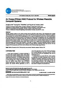
2. Network architecture In this paper, we consider the underwater uplink communication network, in which a surface buoy or a sink node works as a common receiver to collect data from a group of underwater static users, as shown in Fig. 1. Such networks are usually used for the offshore instrument (e.g. wind farm and oil pipeline) health monitoring, underwater data collection and target detection [17]. We assume that each user transmits with the orthogonal frequency-division multiplexing (OFDM) modulation scheme, which has the ability to cope with severe frequency-selective fading due to multipath in underwater channel [18].
Figure 1: An underwater multi-user uplink communication network, where the surface buoy works as the receiver to collect the data from the bottom nodes u1 to u5 .
Due to the size limitation and the high costs associated with underwater instruments, we suppose that each bottom node in UANs equips with a single transducer. We also assume that the receiver has multiple hydrophones for data reception, since the size of a surface buoy is usually much larger than an underwater node. Now denote the number of hydrophones on the buoy and the amount of underwater users in the coverage of the buoy as Mr and L, respectively. Let K denote the maximum number of decodable packets in simultaneous receptions at the receiver, where 4
K ≤ L. We start from a general case of multi-user uplink networks first, where each user can have N transducers with N ≥ 1. Denote the circularly symmetric complex Gaussian noise at hydrophone i of the receiver as ni ∈ CMr ×1 , where ni ∼ N (0, I) and let H†i ∈ CMr ×N be the channel matrix of user i. By using the successive decoding scheme [19] in the multiuser multiple input multiple output (MIMO) uplink communications, the sum-rate capacity of the channel with transmission power constraints P = (P1 , . . . , PK ) is given as [20] K X Cuplink (H1 , . . . , HK , P) = max log I + H†i Qi Hi , Tr(Qi )≤Pi ,∀i
(1)
i=1
where each of the matrices Qi is an N × N positive semidefinite covariance matrix. After the derivation, the sum-rate of the successive decoding in (1) can be written as [21]: Cuplink (H1 , . . . , HK , P) ≤ min (Mr , K) CT DM A (H1 , . . . , HK , P), where
K X CT DM A (H1 , . . . , HK , P) ≥ log 1+ Pi ||Hi ||2
(2)
! ,
(3)
i=1
is the maximum average rate that can be achieved by time division scheme between single-user transmissions with constant power Pi . From (2) and (3) we have that when N = 1, in order to maximize the sum-rate capacity of an underwater multi-user uplink network, the number of packets simultaneously arrived at the receiver should be equal to the amount of hydrophones, i.e., K = Mr . Here we call K < Mr and K > Mr as the starving reception and the supersaturated reception, respectively, both of which may degrade the throughput and the energy efficiency of a network.
3. Motivation In conventional multi-user uplink MAC protocols, people usually use either the handshake or the feedback mechanism to avoid the starving and the supersaturated receptions [8, 9]. However, both mechanisms may work inefficiently in underwater environments due to the following reasons. (a) Collisions among control packets: In acoustic modems, a preamble sequence is embedded in each outgoing packet for the purpose of automatic-gain-control (AGC), packet detection and channel estimation. When taking into account the preamble signal, the lengths of control 5
packets in UANs is usually more than half a second [11], three orders of magnitude longer than that in terrestrial networks. Therefore, collisions among control packets in the handshake process become non-negligible. Especially in a high traffic load scenario, the high collision probability among control packets may significantly degrade the network performance in terms of throughput and energy efficiency. (b) Lack of instantaneous CSI: In multi-user uplink communications, the instantaneous CSI (e.g., the multipath response, channel gain and receiving SNR) is commonly used for adaptive transmission to optimize the communication performance [22, 23]. However, in oceans the instantaneous CSI may not be available due to the long packet transmission time, large propagation delay and high dynamic of acoustic channel [24]. With these three features, there could be a large divergence between the estimated channel state at the transmitter side and the actual one when a packet arrives at the receiver. (c) Unexpected reception: In a terrestrial multi-user uplink network, packets sent in the same slot can arrive at the receiver simultaneously in light of the ignorable propagation delays. However, in underwater networks due to the low propagation speed of the acoustic signal, packets sent by different users simultaneously may arriver at the receiver at different time, and vice versa. Thus the number of packets received by the receiver may be different from the number of active senders. An example is shown in Fig. 2. Assume the surface buoy can decode at most three overlapped packets. The distances from the surface buoy to sender u1 , u2 , u4 and u5 are 1500 m, 1500 m, 750 m and 750 m, respectively. The duration of each data packet is 0.5 s. If the senders u2 and u4 are arranged to send data after the transmission of u1 and u5 , there are only two active senders at each time slot. In radio networks with negligible propagation delays, there are only two packets received by the receiver in each time slot. However, since senders u1 and u5 to the surface buoy have 0.5 s longer propagation delay than u2 and u4 in water, all packets from the four users arrive at the receiver at the same time, causing a supersaturated reception. We call it as the unexpected reception problem, which potentially degrades the throughput and the energy efficiency of underwater networks. (d) Low propagation speed: The sound speed in water is only about 1500 m/s, five orders of magnitude lower than the electromagnetic wave in air. The low acoustic speed may cause the following problems to conventional multi-user uplink MAC protocols.
6
P1
Packet send by u1
p2
Packet send by u2
P4
Packet send by u4
p5
P1
Packet from u1
p2
Packet from u2
P4
Packet from u4
p5
Packet send by u5 Packet from u5
P2 P4
r
P1
P2
P5
P4
P1
r
0.5 s
t 0.5 s
u2 u4
P4
t 0.5 s
u2 u4
P2
P2 P4 0.5 s
t
u1 u5
P5
1s
t
0.5 s
u1 u5
P1 P5
Slot 1
Slot 2
t
0.5 s
P5
Slot 1
Slot 2
Slot 3
t
Underwater acoustic network
Radio networks
Figure 2: Unexpected reception problem in underwater multi-user uplink communication networks, where r is the surface buoy and ui is the user i in Fig. 1.
• Low channel utilization: In a handshake or feedback based multi-user uplink MAC, the time spend on waiting for the control packets is considerable because of the low propagation speed of acoustic signal. This greatly reduces the channel utilization of these protocols. • Fairness issue: In an underwater multi-user uplink network, the difference of propagation delays between the receiver and different senders cannot be ignored anymore. If we use protocols proposed for the terrestrial network, like [8] and [9] in oceans, a user further from the receiver needs to wait a longer time to get a response (handshake or feedback message) than the closer one. In this case, the transmission opportunities for different users are heterogeneous, which leads to a fairness problem. The aforementioned problems motivate us to propose a new MAC protocol for underwater multi-user uplink networks with fair data transmissions, high channel utilization, small end-to-end delay and low energy consumption. 4. CT-MAC protocol In CT-MAC, we suppose that the network is time synchronized1 , which can be done by using the approach proposed in [25] at the initial stage of a network. In this section, we first introduce 1
The overhead of time synchronization in UANs is much higher than that in radio networks. However, the collision
free data transmission and the high channel utilization of CT-MAC could compensate for the additional overhead on running a time synchronization protocol.
7
how CT-MAC works in one-dimensional uplink networks. Then we extend the protocol to the two-dimensional scenario. 4.1. One-dimensional uplink networks A typical one-dimensional network is a string topology network, where acoustic nodes are deployed in a line, as shown in Fig. 1. This topology is widely envisioned in the oil pipeline monitoring and coastline protection systems. In CT-MAC, the time is divided into slots with equal length. Each time slot consists of a competition cycle and a data transmission cycle. 4.1.1. Competition cycle In the competition cycle, each user performs the following three tasks: (a) Generate a random value2 as a priority level (PL) to compete for a sending opportunity. If a user does not have any packet to send, it sets its PL as zero. (b) Deliver the PLs to its direct neighbors instead of broadcasting to the whole network to reduce the energy consumption. (c) If a user has received PLs from its neighbors in previous competition cycles, it works as a helper to relay these PLs in the current competition cycle. In a certain competition cycle, if all users know the PLs of all others, they can decide to send their data or not independently in the following data transmission cycle by comparing the value of corresponding PLs. It is easy to have that with the multihop transmission, a PL requires at most L − 1 time slots to propagate to the whole network, where L is the number of users in a string network. In conventional MAC protocols, the competition is processed in a serial fashion, where a new round of competition will not start until the old one is completed. A typical example is the handshake based MAC, in which a user sends a request-to-send (RTS) packet to its intended receiver and waits for the response, e.g. a clear-to-send (CTS) packet. During the waiting time, even if this user generates a new data packet to the same receiver, it could not initiate a new round of competition until the previous handshake process is ended. 2
More advanced competition schemes for fair transmissions will be introduced in Section 5.
8
If we use the serial competition scheme in CT-MAC, the channel utilization will be very low, since each competition needs L−1 time slots for PLs propagating to the whole network. Therefore, we propose a parallel competition scheme for our protocol. In this scheme, the competition is continuous. Even if the PLs produced by a user in previous time slots have not yet reached the whole network, new PLs will still be generated and sent in each competition cycle. More specifically, let CCi and TCi denote the competition cycle and the data transmission cycle of the ith time slot, respectively. Denote PLi,j as the PL generated by user j in CCi . In Fig. 3, we use three users as an example to show the details of PL propagation in our parallel competitions. In CC1 , the PL produced by each user in the first time slot is only known by the most direct neighbors. Starting from CC2 , users in the network not only generate and transmit new PLs in the current competition cycle, but also help relay old PLs which they received in the previous competition cycle to their neighbors. It is easy to observe that in CC2 , all PLs produced in CC1 are available to all users.
User2
User1
User3
CC1: PL1,1
PL1,2
PL1,1
PL1,2
PL1,3
PL1,2
PL1,3
PL1,1 CC2: PL2,1
PL1,2 PL2,2
PL1,3
PL1,1 PL2,1
PL1,2 PL2,2
PL1,3 PL2,3
PL1,1
PL1,2 PL2,2
PL1,3 PL2,3
PL1,1 PL2,1 CC3: PL3,1
PL1,2 PL2,2 PL3,2
PL1,3 PL2,3
PL1,1 PL2,1 PL3,1
PL1,2 PL2,2 PL . 3,2
PL1,3 PL2,3 PL3,3
PL1,1 PL2,1
PL1,2 PL2,2 PL . 3,2
PL1,3 PL2,3 PL3,3
. . .
. .
. .
Figure 3: The PL transmission scheme in CT-MAC, where the red, blue and black colors represent the newly generated PLs, the overheard PLs from direct neighbors and the historical PLs, respectively.
In general, if there are L users in a one-dimensional uplink network, PLs generated at CCi can be received by all users at CCi+L−2 . This implies that in the first L − 2 time slots of CT-MAC, no user can transmit without a common view on PL competitions. We call these L − 2 time slots as the delaying slots. Since users in CT-MAC need to help relay the PLs from others, a user may push out multiple PLs in one competition cycle. Here we assume in CCi , user j puts all PLs it needs to send in the current competition cycle into the competition packet (CP), CPi,j . In order to avoid collisions among CPs, each user does a random backoff before sending the CP. 9
Transmitted CP
Competition Cycle
User 1
1
Transmitted CP
Received CP
Competition Cycle
Data Transmission Cycle
User 1
Data
2
1
Data
2
t
t User 2
2
1
User 2
Data
3
3
4
User 4
4
5
t 3
2
Data
4
Random Backoff
User 4
Data
3
Data
3
y
t
Waiting Time
1
User 3
Data
2
Random Backoff
2 x
t User 3
4
t
5
3
Data t
t User 5
5
User 5
Data
4
Received CP
Data Transmission Cycle
t
5
Data
4
Slot Beginning Time
(a) TS 1
t
(b) TS 2
Figure 4: Comparison between two transmission schemes.
4.1.2. Transmission cycle To avoid the supersaturated reception, only K out of L users with the highest PLi−L+2,j are allowed to send their data in TCi , where i = L−1, L, L+1, . . . and j = 1, 2, . . . , L. The symbols we used in this paper are described as follows: • c as the sound speed in water, • di as the distance between the receiver and sender i , • tcc as the length of a competition cycle, • ttc as the length of a data transmission cycle, • Ts as the length of a time slot (sum of tcc and ttc ), • tcp as the transmission time of a CP, • tbo as the maximum time of a random backoff, • tdp as the transmission time of a data packet, • li,j as the distance between sender i and sender j, • lmax as the maximum distance between any two neighboring users, • ∆dmax as the maximum difference between distances from the receiver to any two neighboring users. Here di , li,j can be measured at the initial stage of a network by using a classic two-way handshake method, which is generally used in sender–receiver based time synchronization protocols [25]. Similar distance measurement approach has been successfully tested in the sea experiment [26]. lmax and ∆dmax are available at the receiver based on the measurements of di and li,j , respectively. 10
It is worth noting that CT-MAC cannot work in the highly mobile networks. In a mobile network, the distance among users changes with time, indicating the length of competition cycle in CT-MAC needs to be updated frequently. However, CT-MAC measures the distance at the initial stage of a network. Once the protocol starts, the length of competition cycle will remain unchanged. In addition, to eliminate the impact of the error in distance measurements, a guard time is necessary between any two neighboring time slots. In CT-MAC, we want to make packets from different users arrive at the receiver simultaneously.3 In this way, the unexpected reception described in Section 3 could be avoided. To achieve this goal, we design two transmission schemes for our protocol. • Transmission Scheme 1 (TS1 ): All users in TS1 start their time slots concurrently. To make packets from different senders reach the receiver at the same time, the user with a shorter di should wait for the one with a larger di before its data transmission, as shown in Fig. 4(a). Using five users in Fig. 1 as an example, the distance between u3 and the receiver is the shortest among the five users. The waiting time of u3 before its data transmission should be max {di − dj }/c, where i 6= j and i, j = 1, 2, . . . , L. Hence, the minimum ttc and tcc are max {di − dj }/c + tdp and lmax /c + tcp + tbo , receptively. Finally, we have Ts1 = tcc + ttc =
max {di − dj } + lmax + tdp + tcp + tbo . c
(4)
• Transmission Scheme 2 (TS2 ): Different from TS1 , we allow users in TS2 to start their time slots at different time for more efficient data transmissions. As shown in Fig. 4(b), a user with a larger di starts its time slot ahead of a user with a smaller di . For user i, the advanced time of its time slot, which is denoted as xi , is xi = (di − min{dj })/c, where j = 1, 2, . . . , L. With this scheme, we have ttc = tdp . The minimum tcc should be tcc = (∆dmax + lmax )/c + tcp + tbo to guarantee that the competition cycle is long enough for all CPs reception. Finally, we have Ts2 = tcc + ttc =
(∆dmax + lmax ) + tdp + tcp + tbo . c
(5)
In TS2 , since users do not start their time slot at the same time, the competition cycle of a user may overlap with part of the data transmission cycle of its neighbors. Therefore we should 3
If packets from different users arrive at the receiver not exactly at the same time, the packets are still decodable,
but with degraded decoding performance. The research on the misalignment symbol timing of OFDM based multiuser uplink communications can be found in [5] and [7].
11
ensure that there are no sending–receiving collisions between data packets and CPs. Using u1 and u2 in Fig. 4(b) as an example, if a CP from u1 arrives at u2 earlier than the slot beginning time of u2 , i.e., y < x, the reception of this CP may conflict with u2 ’s data transmission. Next, we prove that this collision does not happen in CT-MAC. Proof: y ×c = l1,2 , and x×c = d1 −d2 . Let users u1 , u2 and the receiver be the three vertexes of a triangle, then l1,2 , d1 and d2 are three sides of this triangle. According to the triangle inequality principle that the sum of the lengths of any two sides of a triangle always exceeds the length of the third side, we have l1,2 + d2 > d1 . Hence, we have l1,2 > d1 − d2 , i.e., y > x. � Compared with TS1 , the length of each time slot in TS2 is reduced by max {di − dj }−∆dmax , which improves the channel utilization of the protocol. Finally, the channel utilization of CT-MAC with TS2 , which is denoted as U , is U=
Kc tdp Kttc = . Ts ∆dmax + lmax + c (tdp + tcp + tbo )
(6)
It is worth noting that in the conventional single-input single-output (SISO) network, the channel utilization is less than one. However, in multi-user network, this value may be larger than one, since the network supports multiple users to send their data at the same time without any collision. 4.2. Two-dimensional uplink networks CT-MAC can be easily extended to two-dimensional uplink networks. Its competition mechanism in a two-dimensional network is the same as it in one-dimensional networks. By using the parallel competition scheme, K out of L users with the highest PLs are allowed to send their data in each data transmission cycle. However, in order to transmit CPs efficiently while avoiding the supersaturated reception in a two-dimensional network, the transmission scheme TS2 , which is originally designed for one-dimensional networks, needs a slight modification. In a two-dimensional network, we divide the coverage area of a receiver into several concentric rings, as shown in Fig. 5. The width of each rings is equal, which is denoted as W . Now, we set W = davg , where davg is the average distance between neighboring users in the two-dimensional network. Let ri and d0i denote the ith ring and the average distance from the receiver to users in the ith ring, respectively. Since the distances between the receiver and users in the same ring are close, all users in the same ring start their time slot at the same time. Moreover, users in an outer ring start their 12
1st Ring 2nd Ring 3rd Ring 4th Ring
Cr
W
Figure 5: A general two-dimensional uplink network, where the coverage of the receiver is a cycle with the radius Cr .
time slots earlier than the ones in an inner ring with an advanced time depending on the distance difference to the receiver. Referring to TS2 in Section 4.1.2, the advanced time of users in the ring ri , which is denoted as x0i , is x0i = (d0i − min {d0i })/c. Similar to TS2 in a one-dimensional network, a random backoff before each transmission of CP is also required in the two-dimensional network to avoid collisions among CPs. Therefore, in each competition cycle, a user can successfully receive CPs from its neighbors not only in the same ring but also in the neighboring rings. If there are no isolated users, PL produced by each user can propagate to the whole network within several delaying slots, the number of which is less than or equal to L − 2. Let ∆d0max denote the maximal distance difference between the receiver and any two users in different neighboring rings, which can be calculated by the receiver at the initial stage of the network with a two-way handshake approach. Referring to (5) we have that the minimal length of the time slot in a two-dimensional uplink network is Ts =
(d0max + lmax ) + tdp + tcp + tbo . c
(7)
Replacing parameter ∆dmax in (6) with ∆d0max , we can get the channel utilization of CT-MAC in the two-dimensional uplink networks.
5. Competition schemes for fair transmissions To make the flow of CT-MAC easy to understand, in the previous section, a user just compete for sending opportunities with a random PL. However, the network may have the fairness issue with 13
this simple strategy. In this section, we propose two specific competition schemes for CT-MAC, aiming to improve both the short-term and the long-term fairness of the network. 5.1. Homogeneous traffic generation We start from a common scenario that users in a network have homogeneous traffic generation rates. In this network, the number of packets generated by different users are almost the same in a long time period. In a short time, however, the differences may still exist due to the randomness of the traffic generation at each user. Here, we have two goals for the fair transmission: (a) In a network, the more packets a user accumulated in its sending queue, the higher the transmission opportunity it has to achieve the short-term fairness, (b) The total number of packets sent by users are close in a long period to achieve the long-term fairness. In the following two sections we introduce how to design a competition scheme to achieve these two goals. 5.1.1. Short-term fairness If each user use a random value as the PL to compete for the sending opportunities in the data transmission cycle as what we did in Section 4, transmissions in a short time may be unfair, since the PL of each user is independent with the number of packets it accumulated. Therefore, we need to revise the basic competition scheme to improve its short-term fairness in a homogeneous traffic generation scenario. We assume that each user generates its data packets at the beginning of a time slot. Let gi,j 0 be the total number of packets accumulated by user j at the end of ith time slot and the and gi,j 0 is supposed number of new packets generated by user j in the ith time slot, respectively. Here, gi,j
to follow the Poisson distribution with the mean value λj . For a homogeneous traffic generation rates network, we have λj ≡ λ, for j = 1, 2, . . . , L. Therefore, the number of packets accumulated 0 . Now, we define two by user j in the ith time slot, which is denoted as Ai,j , is Ai,j = gi−1,j + gi,j
events: • Successful Competition Event: If user j wins the competition for transmission in the ith time 1 . slot, we call it as a successful competition to user j, which is denoted as Hi,j
• Failed Competition Event: If user j loses the competition for transmission the ith time slot, 0 . we call it as a failed competition to user j, which is denoted as Hi,j
14
In order to achieve the short-term fairness, the goal of a competition scheme is to make the 1 meet conditional transmission probability of Hi,j 1 |A 1 P(Hi,m i,m = x1 ) > P(Hi,n |Ai,n = x2 ), if x1 > x2 .
(8)
To make (8) hold, in each competition cycle of CT-MAC, user j includes not only the PL, but also the number of accumulated packets, i.e., Ai,j , into CPi,j . In the data transmission cycle, K out of L users with the largest Ai,j are allowed to send their data. If several users have the same number of accumulated packets, then they compare the corresponding PLs as described in Section 4 to determine the final data transmission. We denote this competition scheme as CS.1. 5.1.2. Long-term fairness For a network with homogeneous traffic generation rates, the long-term fairness can be measured by the Jain’s fairness index FJ [27]. FJ =
(
PL
L
2 j=1 γj ) , 2 j=1 γj
PL
(9)
where γj is the channel occupancy rate of user j. The transmissions of a network are fair if FJ is close to one; otherwise, it loses the long-term fairness. In Section 9.1, we will show that CTMAC has a good long-term fairness with the competition scheme CS.1 in a homogeneous traffic generation rates network. 5.2. Heterogeneous traffic generation In a network with heterogeneous traffic generation rates, we assume that the traffic generation 0 , follows the Poisson distribution, but λ 6= λ , if i 6= j. rate of user j, namely gi,j i j
According to (8), if we still use CS.1 in CT-MAC, a user with a large λj may always have larger Ai,j in each time slot than a user with a small λj . In this case, users with small λj may lose all competitions and have no chance to send their data, which will be shown in Section 9.1. Therefore, CS.1 is no longer appropriate for the fair transmission in a heterogeneous traffic generation rates network. For this reason, a new competition scheme is required.
15
5.2.1. Short-term fairness To achieve the short-term fairness in a heterogeneous traffic generation rates network, the goal 1 meet of a competition scheme is to make the conditional transmission probability of Hi,j 1 |A = x ) > P(H 1 |A P(Hi,j i,j 1 k,j = x2 ), if x1 > x2 . k,j
(10)
Different from (8), which is the comparison of accumulated packets among different users in the same time slot, (10) is the comparison of accumulated packets for the same user in different time slots. Therefore, (10) guarantees that users with slow increment on accumulated packets (small λ) still have small but not zero transmission opportunity to send their data. In this situation, all users will have a chance to transmit. 5.2.2. Long-term fairness To achieve the long-term fairness in a network with heterogeneous traffic generation, we expect that the average channel occupancy rate of each user is proportional to its traffic generate rate,4 i.e., Kλj E(γj ) = PL . j=1 λj
(11)
From (11) we have that the total channel occupancy rate
PL
j=1 E(γj )
equals to K, which is the
maximum number of packets a receiver can received at the same time. If we design a competition scheme based on (11), all users will have a chance to send their data. Now, we start from E(γj ), where m
m ∞
i=1
i=1 x=0
1X 1 XX 1 1 E(γj ) = lim P(Hi,j ) = lim P(Hi,j |Ai,j = x)P(Ai,j = x). m→∞ m m→∞ m
(12)
1 ) to make (10) hold, e.g. exponential function, Several kinds of functions can be selected as P(Hi,j
step function and liner function. Here we use the step function as an example to design our competition scheme. We make 1, 1 P(Hi,j |Ai,j = x) = αi,j , 0, 4
x > ui,j x = ui,j
(13)
otherwise,
Although here we make E(γj ) ∝ λj , CT-MAC can support arbitrary channel occupancy pattern by modifying P PL Kλj / L j=1 λj in (11) and (14) to Kυj , where j=1 υj = 1 and υj is the target channel occupancy rate of user j.
16
where αi,j and ui,j can be calculated by substituting (13) into (12), i.e., Kλj . P(Ai,j > ui,j )+αi,j P(Ai,j = ui,j ) = PL j=1 λj
(14)
1 |A ) into its In the competition cycle, each user includes both its PL and the value of P(Hi,j i,j 1 |A ) are allowed to CP. In the data transmission cycle, K out of L users with the largest P(Hi,j i,j 1 |A ), then these users compare send the data. If there are multiple users have the same P(Hi,j i,j
their PLs for the final decision. We denote this competition scheme as CS.2. The long-term fairness of CS.2 will be evaluated in Section 9.1. The competition scheme CS.2 requires users in each time slot to calculate their conditional 1 |A ) based on the number of accumulated packets in the sending transmission probabilities P(Hi,j i,j
queue. Next, we introduce an iterative algorithm to calculate this parameter.
Algorithm 1 0 . According to the Poisson distribution of g 0 with mean value λ , Initialization: Let A1,j = g1,j j 1,j
we have P(A1,j = x) =
(λj )x e−λj . x!
(15)
1 |A ). Substitute (15) into (13) and (14) to calculate P(H1,j 1,j
Step 1: P(gi,j ) can be calculated through 1 |A P(gi,j = x) = P(Hi,j 1,j = x+1)P(Ai,j = x+1)
(16)
1 |A = x)]P(A = x). +[1 − P(H1,j i,j i,j 0 0 Step 2: By using Ai+1,j = gi,j + gi+1,j , where gi,j and gi+1,j are independent, we can calculate
P(Ai+1,j ) through 0 ), P(Ai+1,j ) = P(gi,j ) ∗ P(gi+1,j 0 ∼ Pois(λj ). where ∗ is the convolution operator, and gi+1,j
Step 3: Substitute P(Ai+1,j ) into (14) to calculate ui+1,j and αi+1,j . 1 Step 4: Substitute ui+1,j and αi+1,j into (13) to compute P(Hi+1,j |Ai+1,j ).
17
(17)
1 |A ) in each time slot iteratively. By repeating Step 1 to Step 4, users can calculate their P(Hi,j i,j
6. Power allocation The power allocation strategy in a multi-user network aims to decide the appropriate transmission power to maximize the channel capacity. There have been intensive research in this area to optimize the transmission power in both terrestrial and underwater multi-user uplink networks. Since the power allocation is not the focus of this paper, we just give a brief introduction on power allocation in CT-MAC. As we discussed in Section 3, the instantaneous CSI may not be available in underwater communications, due to the large propagation delay, long packet transmission time and high dynamic of acoustic channel. However, the statistical information of underwater channel can be utilized for power allocation, since it is relatively stable in a relative long time period [24]. In CT-MAC, we can measure the statistical information, such as the average receiving SNR and the distribution of channel response, at the initial stage of the network, and then consider it as a priori knowledge. In this way, existing algorithms, such as [23] and [28], can be employed by CT-MAC to decide the optimum transmission power on active senders. It is worth noting that the aforementioned power allocation algorithms usually require the MAC layer to provide the information about which user will transmit. This information is available in CTMAC with its parallel competition scheme, since users completely know who wins the competition for the data sending in each time slot. This is one superior of CT-MAC when compared with some conventional MAC protocols [8, 29].
7. The bad request issue In this section, we introduce a specific issue in CT-MAC, which may degrade the channel utilization of the protocol. To improve the channel utilization, we designed a parallel competition scheme for CT-MAC. 1 |A ) to Essentially, users in this scheme utilize their current statuses, namely Ai,j , PL and P(Hi,j i,j
compete for the transmission opportunities in the future time slots. If their statuses are changed 18
during the propagation of CP, these transmission opportunities may be wasted. We call this problem as the bad request issue. Using a string topology network with 20 users as an example, suppose the traffic generation rates of the network are homogeneous, and the competition scheme CS.1 is employed. Denote the time slot i as Si . We assume that in S1 , user u1 has a data to send. According to CS.1, it sends A1,1 = 1 to its neighbors. However, in the following seventeen slots, even if u1 does not generate any new data, it still produces Ai,1 = 1, i = 2, . . . , 18 to compete for the transmission opportunities in the slots from S2 to S18 . This is because the competition results in S1 are not known immediately but be delayed by 18 slots as described in Section4. Therefore, u1 continually competes the sending opportunity for the single data packet it generated in S1 . After delaying slots, at S19 , we suppose that u1 wins the competition and sends out the only packet it accumulated in the queue. However, u1 has attended all the competitions between S2 and S18 . In this case, u1 wastes the sending opportunities if it wins one or more competitions in these slots, since it currently has no data to send. We will evaluate the impact of the bad request issue on channel utilization of CT-MAC in Section 9.1.
8. The CP loss problem In CT-MAC, CP carries the competition information for each user. The successful transmission of CPs is thus important. Although we have used the backoff mechanism to prevent collisions among CPs, the reception of CP may still fail due to the poor channel quality caused by the high noise level, long multipath or wide Doppler spread. In this section, we first evaluate the effect of the CP loss in one-dimensional networks, and then propose two feasible solutions to handle the lost CPs. 8.1. Effect of CP loss In a string network, the quality of acoustic channels between different neighbors may have some differences. Therefore, we assume that the successful transmission probability (delivery ratio) of CPs also varies on different links. Let pj and p0j be the delivery ratio of the CP from user (j + 1) to user j, and from user j to user (j + 1), respectively, as shown in Fig. 6. Denote Pij as the delivery ratio of a CP from user i 19
U2
U3
UL-2
. . .
U1
UL-1
UL
Figure 6: The delivery ratio of CP in a string network.
to user j, where Q j k=i−1 pk , Pij = 1, Qj−1 p0 ,
i > j, i = j,
(18)
i < j.
k=i k
If a user misses CPi,j , the corresponding competition information, such as PLi,j , Ai,j and 1 |A ), which is carried by this CP, is also lost. Using PL P(Hi,j i,j i,j as an example, let wj denote the
number of lost PLs on user j in a specific cycle. Denote the probability density of wj as P(wj ). It is easy to have that the probability that user j successfully receive all PLs, which are generated in a same competition cycle, is P(wj = 0) =
L Q
Pij .
(19)
i=1
The probability that user j misses one of these PLs is P(wj = 1)=
L L P Q (1−Pij ) Pkj
i=1
k=1 k6=i L Q
L 1−P P ij Pkj P ij k=1 i=1 � � L P 1 = −1 P(wj = 0). i=1 Pij
=
(20)
Then the probability that user j misses two of these PLs is L L L X Q 1X (1−Pij ) (1−Pkj ) Pmj P(wj = 2)= 2! m=1 i=1
k=1 k6=i
m6=i,k
(21)
� L� � �2 � L� X 1 X 1 1 = −1 P(wj =1)− −1 P(wj = 0) . 2 Pij Pkj i=1
k=1
Finally, we can calculate P(wj ) iteratively with the following expression: x
P(wj = x) =
1X (−1)i−1 ψj (i)P(wj = x−1), x i=1
20
(22)
where x = 1, . . . , L and ψj (i) =
L P
1 − 1)i . Pkj
(23)
xP(wj = x).
(24)
(
k=1
The mean value of wj is E(wj ) =
L P
x=1
The analytical expression of the average number of lost PLs in (24) could help us evaluate the performance of CT-MAC in real network easily. If a user misses the competition information from others in a competition cycle, it is unable to accurately decide if it should send data or not in the following data transmission cycle. In the next section, we introduce how to handle this problem. 8.2. Handling the CP loss problem In CT-MAC, we can use two simple strategies, namely, the underestimation and the overestimation, to handle the lost CPs. In the underestimation strategy, if a user loses any other users’ competition information, e.g., 1 |A ) and A , it assumes that these users have the lowest priority in this round of PLi,j , P(Hi,j i,j i,j
competition. It is easy to understand that with the this strategy, the number of active users in each data transmission cycle is possibly larger than the maximum number of senders that a network can support, which causes a supersaturated reception. In the overestimation strategy, a user assumes that the users, the competition information of which are lost, have the highest priority for the data transmission. With this strategy, the channel resource may be wasted, since the number of active users is possibly less than the maximum number of active senders that a network can support if the lost priority information is overestimated, which causes a starving reception. Although the channel utilization is not optimal when the starving reception happens, all packets could be decoded by the receiver successfully as long as the channel is good. By contrast, if supersaturated reception happens, the data packets will collide at the receiver, which is the worst case and should be avoided in underwater communications. For this reason, in CT-MAC we consider the overestimation as a wiser option than the underestimation strategy to handle the lost CPs. Now, we derive the channel utilization of CT-MAC in a homogeneous traffic rates network with the overestimation strategy. In an ideal situation, where there is no lost CP, the average 21
transmission probability of each user in the data transmission cycle is K/L. When taking into account the lost CPs, this probability is reduced to (K − wj )/(L − wj ) for user j. Denote the average number of active users as K 0 , we have K0 =
L P K K −x P P(wj = x), i=1 x=1 L − x
(25)
which is less than or equal to K. Finally, replacing K in (6) with K 0 , we will get the channel utilization of CT-MAC in a network with homogeneous traffic generation rates and under CP loss effect.
9. Simulations and analysis In this section, we use the MATLAB5 as the simulation platform to evaluate the performance of CT-MAC in a string network. The depth of nodes and the distance between neighboring users are 500 m and 200 m, respectively. In the simulation, we use two different sizes of network, L = 10 and L = 20, as examples for performance evaluation. The number of hydrophones on the receiver is Mr = 4. We first evaluate the fairness of different competition schemes, and show the impact of the CP loss problem and bad request issue on CT-MAC in Section. 9.1. Then, we compare CT-MAC with two representative multi-user MAC protocols in terms of the channel utilization, energy efficiency and end-to-end delay in Section 9.2. 9.1. Performance evaluation Firstly, we evaluate the long-term fairness of competition scheme CS.1 in a string network with homogeneous traffic generation rates. For comparison purpose, two different competition schemes, which are denoted as CS.3 and CS.4, are also investigated. In CS.3, K out of L users with the lowest Ai,j are allowed to send their data, which is completely opposite to CS.1. In CS.4, K/2 out of L users with the highest Ai,j , and another K/2 users with the lowest Ai,j are arranged to send their data in each data transmission cycle. This competition scheme can be considered as a mixture of CS.1 and CS.3. 5
Considering the simpleness of multi-user networks with single receiver, using MATLAB is sufficient to simulate
the collision avoidance and transmission scheduling of CT-MAC. Therefore, we did not choose other specialized underwater network simulators, such as Aqua-Sim [30] or SUNSET [31], for performance evaluations.
22
In Fig. 7, we set the traffic generation rate λj = 1 for j = 1, 2, . . . , 20, in a network with 20 senders and plot the Jain’s fairness index FJ for all three competition schemes. From this figure, we observe that FJ of CS.1 is gradually close to one with the running of the protocol. This proves that CT-MAC with CS.1 achieves a good long-term fairness in the network with homogeneous traffic generation rates. By contrast, FJ of CS.3 and CS.4 are very low, close to 0.2 and 0.4, respectively. This implies that CT-MAC loses its long-term fairness with these two competition schemes. In addition, we observe that FJ of all three competition schemes in Fig. 7 starts from 0.2. This is because no matter which competition scheme we used, after the first data transmission, if user j sends the data, γj in (9) always equal to one; otherwise, γj = 0. In each data transmission cycle, there are K users are allowed to transmit. Therefore, FJ of all competition schemes starts from K/L, which is 0.2. 1.2
CS.1 CS.3 CS.4
Fairness index FJ
1 0.8 0.6 0.4 0.2 0
0
50
100 Time slot
150
200
Figure 7: Comparison of the long-term fairness in a network with homogeneous traffic generation rates.
To give us an insight into Fig. 7, we plot the distribution of the number of accumulated packets, i.e., P(Ai,j ), after the protocol ran 10, 000 time slots, as shown in Fig. 8. If none of users in the network send data, then the average number of Ai,j should equal to the number of time slots, which is 10, 000, because λj = 1, j = 1, 2 . . . , L. In this figure, when using CS.1, we observe that Ai,j is distributed around 8000. More specifically, since the data transmission in CS.1 is fair in a long-term period, the packet transmission opportunity of all users are almost equal, which is K/L = 0.2. Therefore, after 10, 000 time slot the average number of Ai,j is (1 − 0.2)×10, 000 = 8000, which proves the long-term fairness of CS.1 again. For comparison, when we use CS.3 in CT-MAC, a user with a larger Ai,j is more likely to fail the transmission competition than a user with a smaller Ai,j . This finally leads to an extremely 23
P(A i, j)
0.02
0.01
0
CS.1
Simulation Result Theorytical Result
0
1000
2000
3000
4000
5000
6000
7000
8000
9000
10000
6000
7000
8000
9000
10000
6000
7000
8000
9000
10000
A i, j
P(A i, j)
0.02
0
CS.3
Simulation Result Theorytical Result
0.01
0
1000
2000
3000
4000
5000
A i, j
P(A i, j)
0.02
Simulation Result Theorytical Result
0.01
0
0
1000
2000
3000
CS.4
4000
5000
A i, j
Figure 8: The distribution of Ai,j in CT-MAC with different competition schemes.
differentiated Ai,j . Part of users, who win first, easily get the chance to send their data later on (Ai,j goes down to zero), and others that failed the competition at the beginning keep losing the sending opportunities in the future competitions (Ai,j goes up to 10,000). The fairness problem also occurs in CS.4, but less severe than that in CS.3. This is because each user in CS.4 has a chance to send its data in each time slot, although the sending opportunities are not equal for all users. More specifically, both users with the largest and smallest Ai,j in CS.4 have transmission opportunities. That is why the left peak of P(Ai,j ) in CS.4 of Fig. 8 is round 9000 rather than 10, 000, and the area of the right part in CS.4 is smaller than that in CS.3. In addition, to test the accuracy of Algorithm 1, we also compare the theoretical analysis of P(Ai,j ) with the simulation results. From the comparisons in Fig. 8 we have that the theoretical computations of P(Ai,j ) match the simulation results very well in all three competition schemes. In a network with heterogeneous traffics, we make λj of different users uniformly distributed between 0.1 and 2 to evaluate the long-term fairness of CS.2. As shown in Fig. 9, the channel occupation rate of λj conforms to (11), which is proportional to the traffic generation rates. By contrast, if we still use CS.1 in the heterogeneous traffic generation rates network, the transmission opportunity of users with small λj may be “plundered” by users with larger λj . This can be found in Fig. 9, where the channel occupancies of the eleven users with lower traffic loads (λj between 0.1 and 1) are almost zero. In Fig. 10, we use a 10 senders network as an example to show the average number of lost PLs 24
at each user with respect to the delivery ratio of CPs, i.e., pj and p0j . From this figure we observe that pj affects E(wj ) significantly. When pj = 0.99, two edge nodes, u1 and u10 , lose 0.5 PLs in average, which is only 5% out of the total. However, when pj reduces to 0.9, the average number of lost PLs at u1 and u10 grows to 3.5, six times higher than that in the case with pj = 0.99. Moreover, the position of a user in the network also affects its E(wj ). Compared with users on the edge of network, users in the central of network have much smaller E(wj ) owing to the less number of hops for CP forwarding. In addition, Fig. 10 also shows the consistence between the simulation results
1
5 4.5
CS.1 0.8
CS.2
Average number of lost PLs
Normalized channel occupancy rate ( γ j )
of lost CPs and the theoretical analysis derived from (22) to (24).
Optimum 0.6
0.4
0.2
Theoretical results: p j = 0.9
4
p j = 0.95
p j = 0.95
3.5
Simulation results: p j = 0.9 p j = 0.99
p j = 0.99
3 2.5 2 1.5 1 0.5
0
0
0.5 1 1.5 Traffic generation rate of users ( λ j )
0
2
Figure 9: The long-term fairness.
2
4
6 User ID
8
10
Figure 10: The average number of lost PLs.
Fig. 11 demonstrates the impact of lost CPs on CT-MAC, where the overestimation strategy is employed. We observe an improvement on the channel utilization as the size of the network reduces and the delivery ratio of CPs increases. This figure reveals that the multi-user uplink network with a larger number of users is much more sensitive to the CP loss than a network with smaller size. When reducing p from 1 to 0.9, the throughput degrades by 60% for the network with 10 users, compared with 99% reduction for the network with 20 users. Therefore, a larger size of a network requires a higher reliability on CP transmission in CT-MAC. Again, the validity of the theoretical analysis on the channel utilization of CT-MAC under the effect of CP loss is confirmed by comparing with simulation results. As shown in Fig. 11, the theoretical results derived from (6) and (25) match the simulation results very well. In Fig. 12, we evaluate the effect of the bad request issue on CT-MAC. In the ideal situation, we suppose that users in the simulation get aware of all Ai,j information immediately. To compare with this ideal case, we plot the channel utilization of CT-MAC in the real scenario, where L − 2 25
1
Theoretical results: Simulation results: L=10 L=10 L=15 L=15 L=20 L=20
1 Normalized channel utilization
Normalized channel utilization
1.2
0.8 0.6 0.4 0.2 0 0.9
0.92
0.94
0.96
0.98
0.8
0.6
0.2
0
1
pj
Figure 11: Channel utilization with respect to pj .
L=10, optimum situation L=10, with bad request L=15, optimum situation L=15, with bad request L=20, optimum situation L=20, with bad request
0.4
0
0.05 0.1 0.15 Traffic generation rate ( λ )
0.2
Figure 12: Effect of the bad request.
delaying slots exist in the protocol. From Fig. 12 we observe that the bad request problem slightly degrades the channel utilization especially in a large network, where the PL information need more time slots to propagate to the whole network, and the number of packets accumulated by each user has high probability to change during the propagation of PLs. If users have competed more transmission opportunities than they need, the bad request incurs and degrades the network throughput. In addition, with the increment of traffic generation rates, the negative effect of bad request issue becomes negligible. This is because in a high traffic network, the amount of accumulated packets on each user has small chance to be zero, thus reducing the probability to waste transmission opportunities. 9.2. Performance comparison To verify the advantages of CT-MAC on channel utilization, energy efficiency and end-to-end delay, we compare CT-MAC with two representative multi-user MAC protocols, namely, channel aware Aloha [8] and multi-antenna reception MAC [9], both of which were briefly introduced in Section. 1. Here, the channel utilization is defined as the ratio of the channel resource utilized for successful data transmissions,6 which can be a value larger than one in multi-user uplink networks. The energy efficiency is measured as the average power consumption on both control and data transmissions per each successful data delivery. The end-to-end delay measures the average delay for a data packet to be delivered to the surface receiver. 6
The network throughput can be represented as the channel utilization times data transmission rate.
26
The default network size we used in the following simulations is L = 10. The duration of a preamble signal in each packet is 0.5 s, which is the same as the real acoustic modem [11]. The lengths of data and CP are 400 bytes and 40 bytes, respectively. The transmission rate of acoustic modems is 3 kbps. We use Rayleigh fading
7
to model the acoustic channel with mean value
βj [34], where βj is proportional to the square of communication range, d2j . The default successful transmission rate of CPs is set as pj = p0j , 0.98
8
for j = 1, 2, . . . , L − 1. The performance of
CT-MAC with different pj is also evaluated. Since the receiver in our simulations can support a maximum of 4 simultaneous transmissions, the upper-bound of the channel utilization is 400%. From Fig. 13(a) we observe that the channel utilizations of all three MAC protocols are close in low traffic scenarios (0 ≤ λj ≤ 0.02). This is because with a small λj , users in all protocols have enough time to send out the generated packets. The channel utilization in this case is constrained by the traffic generation rate. However, with the growth of traffic rate, CT-MAC demonstrates remarkably higher channel utilization than the two representative MAC protocols, because the parallel competition mechanism of CT-MAC can avoid starving and supersaturated receptions with very low latency. By contrast, the poor collision avoidance ability of channel aware Aloha and the high latency of the handshake process in multi-antenna reception MAC lead to low channel utilizations. We suggest that CT-MAC outperforms the random access based channel aware Aloha and handshake based multi-antenna reception MAC in terms of channel utilization. In Fig. 13(b), we use the energy consumption coefficient to evaluate the energy efficiency of the protocols. The energy consumption coefficient is calculated as the energy consumption on sending a single data packet dividing the total energy consumed on each successful data delivery, which takes the collision and control packet overhead into account. A high energy consumption coefficient stands for a low energy efficiency of a protocol. As revealed in Fig. 13(b), the energy efficiency of CT-MAC is considerably lower than the other two protocols if the traffic rate is lower than 0.038 packets per second. In the low traffic rate 7
There have been extensive studies on modeling underwater horizontal channel [32, 33, 34]. However, the models
of underwater vertical channel are still rare. The impact of different channel models on performance of the protocols will be discussed at the end of this section. 8 According to the long term experimental results we collected at the Long Island Sound, the average delivery ratio of short packets can achieve at least 95% for the middle range (556 m) shallow water OFDM communications [35]. Higher delivery ratio can be expected for CP transmissions due to the shorter distance (200 m) and deeper water communication environments.
27
6
2 1.5 1 0.5 0
0
0.05 0.1 0.15 Traffic rate per user
(a) Channel utilization
0.2
Channel aware Aloha Multi−antenna reception MAC CT−MAC
8 6
10
Channel aware Aloha Multi−antenna reception MAC CT−MAC
4
10
Delay (s)
Channel aware Aloha Multi−antenna reception MAC CT−MAC
Energy consumption coefficient
Channel Utilization
2.5
4
2
10
2 0
0
0
0.05 0.1 0.15 Traffic rate per user
(b) Energy efficiency
0.2
10
0
0.05
0.1 0.15 Traffic rate per user
0.2
(c) Delay
Figure 13: Performance comparisons among the three protocols with pj = 0.98.
situation, even if a node does not have any data to send, it still needs to transmit and forward PL information in each time slot. Therefore, the large overhead on CP transmissions results in a high energy consumption coefficient for CT-MAC at low traffic rates. However, with the growth of traffic rate, CT-MAC achieves comparable or even better energy efficiency than channel aware Aloha. The channel aware Aloha has low energy consumption because it only allows users with the best channels to send their data, which significantly improves the energy efficiency. However, the fairness issue will be a problem, as a user with bad channel (e.g., the user at the edge of a network) has less chance to send its data than a user with a good channel quality. The multi-antenna reception MAC has the highest energy consumption among the three protocols due to the heavy overhead on broadcasting and retransmitting the control packets through long distance links. Fig. 13(c) illustrates the end-to-end delays of the three protocols. When the traffic rate is lower than 0.038 packets per seconds, the end-to-end delays of both CT-MAC and muti-antenna reception MAC are around 4.9 s, whereas channel aware Aloha has 9.5 s by contrast. In CTMAC and muti-antenna reception MAC, the end-to-end delay at low traffic loads consists of the transmission time of control and data packets, and the propagation delay. Channel aware Aloha has extra delays waiting for the channel going good, since only users with the good channels are allowed to transmit. This explains why there are large delays in the channel aware Aloha with low traffic loads. When the traffic load goes heavy, the end-to-end delays of all protocols shapely increase as the channel starts to saturate. However, for different MAC protocols, the saturated traffic rates are different. Owing to the high channel utilization, CT-MAC can afford a much higher 28
traffic rate than the other two protocols without overwhelming the acoustic channel, which results in the lowest end-to-end delay. It is worth noting that the channel model we used in Fig. 13 is Rayleigh fading channel. This model is appropriate for the channels between the surface buoy and its furthest users, which are horizontal channels. For users underneath the buoy, the vertical channel has much less multipath, and the channel model, such as Rice [32] and Gaussian fading [34], may be more appropriate than the Rayleigh model. When the channel model used in simulations does not fit the channel in the real environment, the channel utilization of channel aware Aloha may be different from what we illustrated in Fig. 13, since the transmission strategy of this protocol is optimized based on the Rayleigh model. In addition, although the design of CT-MAC and muti-antenna reception MAC is independent with the channel model we are using, it still affects the performance of these two protocols by affecting their packet (data or CP) loss ratio. Table 1: Performance of CT-MAC with respect to the delivery ratio of CP (pj ). L = 10
L = 20
Max channel utilization
Min energy consumption
Max channel utilization
Min energy consumption
pj
Value
Percentage
Value
Percentage
Value
Percentage
Value
Percentage
1
1.94
100
7.02
100
1.84
100
6.84
100
0.98
1.73
89.18
7.18
102.24
1.15
62.19
7.35
107.42
0.95
1.39
71.37
7.55
107.49
0.18
9.53
14.33
209.40
0.93
1.15
59.15
7.89
112.27
0.08
4.24
23.80
347.94
0.9
0.83
42.67
8.73
124.24
0.04
2.33
40.09
585.98
The significant effect of CP loss on the performance of CT-MAC has been illustrated in Fig. 11. In order to give an insight into this problem, we compare the maximum channel utilization and the minimum energy consumption coefficient of CT-MAC with respect to different CP delivery ratios, and list the results in Table 1. The percentage values are relative to the situation with no CP loss (pj = 1). On the one hand, the channel utilization of CT-MAC is remarkably affected by pj . When pj decreases from 1 to 0.95 for L = 10, the channel utilization reduces by about 30%. It is acceptable as the performance of CT-MAC in this case is still better than the channel aware Aloha and multi-antenna reception MAC. However, when pj continuously decreases to 0.9 for L = 10, the degradation on channel utilization will be too high to work efficiently, due to the significant CP loss. On the other hand, the energy efficiency is less affected by pj . Compared with the scenario of no CP loss, only 20% additional energy is consumed when pj = 0.9. This is because the lost 29
CPs do not increase the collision of data packet with overestimation scheme. From Table 1 we also observe that CT-MAC cannot work well in a large size network with low CP delivery ratio. For L = 20, CT-MAC cannot work efficiently when pj is lower 0.98. When pj = 0.9, most of PLs are lost by users and no data could be sent, which results in the channel utilization reducing by 97% and the energy consumption increasing by 486%. 6
5
10
10 pj=1.00 pj=0.98
5
10
4
10
pj=0.95 4
10
pj=0.90
pj=0.98
3
Delay (s)
Delay (s)
pj=1.00
pj=0.93
3
10
10
pj=0.95 pj=0.93 pj=0.90
2
10
2
10
1
10
1
10
0
10
0
0
0.05
0.1 0.15 Traffic rate per user
10
0.2
(a) L=10
0
0.05
0.1 0.15 Traffic rate per user
0.2
(b) L=20
Figure 14: Delay of CT-MAC with respect to the delivery ratio of CP and traffic generation rate.
In Fig. 14, we show the end-to-end delays of CT-MAC with respect to the delivery ratio of CPs and traffic generation rate. It is easy to observe that the delays have sharp increase when the traffic load reaches to a certain threshold. In another word, when the traffic generation rate exceeds the throughput a network, tremendous packets will be accumulated and cause considerable end-to-end delays. The increase of CP loss ratio reduces the channel utilization of CT-MAC, which results in a lower threshold, as shown in Fig. 14. For example, when L = 10 and pj = 1, the end-to-end delay increases significantly if traffic rate higher than 0.12. This threshold is reduced to 0.038 when pj = 0.9. Moreover, when considering the lost CPs, a large size network (L = 20) has incredibly long delays at low traffic rates. It can be observed by comparing the traffic rate thresholds in Fig. 14(a) with that in Fig. 14(b). This is because a larger network has more PL losses in average than a smaller network, causing considerable waste of data transmission opportunities in overestimation scheme. The degraded channel utilization of CT-MAC makes the packet cannot be sent out timely and leads to long end-to-end delays. The results in Table 1 and Fig.14 reveal the fact that the reliable transmission of CP is crucially important to CT-MAC, especially in a large size network. In order to guarantee the efficiency of 30
this protocol, the feasible solutions include (a) increasing the reliability of CP delivery, especially in a large size network, and (b) dividing the large network into small ones, and let each subnetwork runs CT-MAC in parallel.
10. Conclusions In this paper, we presented a competitive transmission MAC (CT-MAC) for underwater multiuser uplink communication networks. In CT-MAC, the unique features of underwater acoustic systems, such as the long propagation delay, low transmission rate and long preamble of acoustic modem are considered carefully. To improve the channel utilization, the energy efficiency and end-to-end delay, users in CT-MAC use a parallel competition scheme to compete for the data transmission opportunities. With this scheme, data generated by users in different time slots can join the transmission competitions in parallel, and the control packets from each user only need to reach its direct neighbors instead of the whole network. Additionally, two competition schemes are proposed for the fair transmission in networks with both homogeneous and heterogeneous traffic generation rates. Moreover, two specific problems, namely, the bad request issue and the lost competition packet (CP) problem in CT-MAC are studied. The solutions to address these problems are also proposed in this paper. Finally, we evaluate the performance of CT-MAC through theoretical analysis and simulations. Compared to the channel aware Aloha and the multi-antenna reception MAC, CT-MAC has higher channel utilization under a wide range of traffic generation rates. Especially in a high traffic scenario, the channel utilization of CT-MAC is about 3.15 and 3.4 times higher than the channel aware Aloha and the multi-antenna reception MAC, respectively. Moreover, the energy consumption per each successful data transmission of CT-MAC at the high traffic rates also outperforms the other two protocols. Finally, CT-MAC has remarkably lower end-to-end delay than the channel aware Aloha and the multi-antenna reception MAC, as the high channel utilization allows CT-MAC to send packets in a much faster way without overwhelming the acoustic channel. However, the performance of CT-MAC considerably relay on the reliable transmission of CP. Once the delivery ratio of CP is low, the performance of CT-MAC will degrade significantly, which should be avoided in the real applications.
31
Acknowledgments This work is supported in part by the US National Science Foundation under Grant Nos.1018422, 1127084, 1128581, 1205665, 1208499, and 1331851.
References [1] I. F. Akyildiz, D. Pompili, T. Melodia, Underwater acoustic sensor networks: research challenges, Ad Hoc Networks 3 (3) (2005) 257–279. [2] J.-H. Cui, J. Kong, M. Gerla, S. Zhou, The challenges of building mobile underwater wireless networks for aquatic applications, IEEE Network 20 (3) (2006) 12–18. [3] Y. Luo, L. Pu, M. Zuba, Z. Peng, J.-H. Cui, Challenges and opportunities of underwater cognitive acoustic networks, IEEE Transactions on Emerging Topics in Computing 2 (2) (2014) 198–211. [4] M. Stojanovic, On the relationship between capacity and distance in an underwater acoustic communication channel, ACM SIGMOBILE Mobile Computing and Communications Review 11 (4) (2007) 34–43. [5] M. Park, K. Ko, H. Yoo, D. Hong, Performance analysis of OFDMA uplink systems with symbol timing misalignment, IEEE Communications Letters 7 (8) (2003) 376–378. [6] A. L. Hui, K. Letaief, Successive interference cancellation for multiuser asynchronous DS/CDMA detectors in multipath fading links, IEEE Transactions on Communications 46 (3) (1998) 384–391. [7] Z. Wang, S. Zhou, J. Catipovic, P. Willett, Asynchronous multiuser reception for OFDM in underwater acoustic communications, in: Proceedings of IEEE OCEANS, 2012, pp. 1–6. [8] X. Qin, R. Berry, Exploiting multiuser diversity for medium access control in wireless networks, in: Proceedings of IEEE INFOCOM, 2003. [9] N. Sato, T. Fujii, A MAC protocol for multi-packet ad-hoc wireless network utilizing multi-antenna, in: Proceedings of IEEE CCNC, 2009, pp. 1–5. [10] J. Partan, J. Kurose, B. N. Levine, A survey of practical issues in underwater networks, ACM SIGMOBILE Mobile Computing and Communications Review 11 (2007) 23–33. [11] L. Pu, Y. Luo, Y. Zhu, Z. Peng, J.-H. Cui, S. Khare, L. Wang, B. Liu, Impact of real modem characteristics on practical underwater MAC design, in: Proceedings of IEEE OCEANS, 2012, pp. 1–6. [12] A. Song, M. Badiey, H. Song, W. S. Hodgkiss, M. B. Porter, et al., Impact of ocean variability on coherent underwater acoustic communications during the Kauai experiment (KauaiEx), The Journal of the Acoustical Society of America 123 (2008) 856. [13] L.-C. Kuo, T. Melodia, Distributed medium access control strategies for MIMO underwater acoustic networking, IEEE Transactions on Wireless Communications 10 (8) (2011) 2523–2533. [14] T. Yoo, A. Goldsmith, Capacity and power allocation for fading MIMO channels with channel estimation error, IEEE Transactions on Information Theory 52 (5) (2006) 2203–2214. [15] D. P. Palomar, J. M. Cioffi, M. A. Lagunas, Uniform power allocation in MIMO channels: a game-theoretic approach, IEEE Transactions on Information Theory 49 (7) (2003) 1707–1727.
32
[16] D. Gesbert, M. Shafi, D.-s. Shiu, P. J. Smith, A. Naguib, From theory to practice: an overview of MIMO space-time coded wireless systems, IEEE Journal on Selected Areas in Communications (2003) 281–302. [17] N. Mohamed, I. Jawhar, J. Al-Jaroodi, L. Zhang, Sensor network architectures for monitoring underwater pipelines, Sensors 11 (11) (2011) 10738–10764. [18] B. Li, S. Zhou, M. Stojanovic, L. Freitag, P. Willett, Multicarrier communication over underwater acoustic channels with nonuniform Doppler shifts, IEEE Journal of Oceanic Engineering 33 (2) (2008) 198–209. [19] T. M. Cover, J. A. Thomas, Elements of information theory, John Wiley & Sons, 2012. [20] A. Goldsmith, S. A. Jafar, N. Jindal, S. Vishwanath, Capacity limits of MIMO channels, IEEE Journal on Selected Areas in Communications 21 (5) (2003) 684–702. [21] N. Jindal, A. Goldsmith, Dirty-paper coding versus TDMA for MIMO broadcast channels, IEEE Transactions on Information Theory 51 (5) (2005) 1783–1794. [22] W. Yu, W. Rhee, J. M. Cioffi, Optimal power control in multiple access fading channels with multiple antennas, in: Proceedings of ICC, 2001. [23] A. Soysal, S. Ulukus, Optimum power allocation for single-user MIMO and multi-user MIMO-MAC with partial CSI, IEEE Journal on Selected Areas in Communications 25 (7) (2007) 1402–1412. [24] L. Pu, Y. Luo, H. Mo, J.-H. Cui, Z. Jiang, Comparing underwater mac protocols in real sea experiment, in: Proceedings of IFIP Networking, 2013. [25] A. A. Syed, J. S. Heidemann, Time synchronization for high latency acoustic networks, in: Proceedings of IEEE INFOCOM, 2006. [26] S. N. Le, Y. Zhu, J.-H. Cui, Z. Jiang, Pipelined transmission MAC for string underwater acoustic networks, in: Proceedings of ACM WUWNet, 2013. [27] R. Jain, The art of computer systems performance analysis, John Wiley & Sons, 1991. [28] W. Rhee, J. M. Cioffi, Ergodic capacity of multi-antenna Gaussian multiple-access channels, in: Conference Record of the Thirty-Fifth Asilomar Conference on Signals, Systems and Computers, IEEE, 2001. [29] L. X. Cai, H. Shan, W. Zhuang, X. Shen, J. W. Mark, Z. Wang, A distributed multi-user mimo mac protocol for wireless local area networks, in: Proceedings of IEEE GLOBECOM, 2008, pp. 1–5. [30] Y. Zhu, X. Lu, L. Pu, Y. Su, R. Martin, M. Zuba, Z. Peng, J.-H. Cui, Aqua-Sim: an NS-2 based simulator for underwater sensor networks, in: Proceedings of ACM WUWNet, 2013. [31] C. Petrioli, R. Petroccia, SUNSET: Simulation, emulation and real-life testing of underwater wireless sensor networks, in: Proceedings of IEEE UComms, 2012, pp. 12–14. [32] F. Ruiz-Vega, M. C. Clemente, P. Otero, J. F. Paris, Ricean shadowed statistical characterization of shallow water acoustic channels for wireless communications, arXiv preprint arXiv:1112.4410. [33] W.-B. Yang, T. Yang, Characterization and modeling of underwater acoustic communications channels for frequency-shift-keying signals, in: Proceedings of IEEE OCEANS, 2006, pp. 1–6. [34] M. Chitre, J. Potter, O. S. Heng, Underwater acoustic channel characterisation for medium-range shallow water communications, in: Proceedings of IEEE OCEANS, 2004, pp. 40–45. [35] Y. Luo, L. Pu, Z. Peng, Z. Shi, J.-H. Cui, Exploring RSS Based Secret Key Generation in Underwater Acoustic Networks with Sea Experiments, Tech. Rep. Technical Report: UbiNet-TR14-01, UCONN CSE (2014).
33