recognition experiments with TIMIT speech corpus. The robustness of ... for speech recognition using real data are presented and discussed. Two different.
An EM Algorithm to Learn Sequences in the Wavelet Domain Diego H. Milone and Leandro E. Di Persia
sinc(i) Research Center for Signals, Systems and Computational Intelligence (fich.unl.edu.ar/sinc) D. H. Milone & L. Di Persia; "An EM algorithm to learn sequences in the wavelet domain" Lecture Notes in Artificial Intelligence, Vol. 4827, pp. 518-528, 2007.
Signals and Computational Intelligence Laboratory - CONICET Department of Informatics, Faculty of Engineering and Water Sciences National University of Litoral, Ciudad Universitaria, Santa Fe, Argentina {dmilone,ldipersia}@fich.unl.edu.ar http://fich.unl.edu.ar/sinc
Abstract. The wavelet transform has been used for feature extraction in many applications of pattern recognition. However, in general the learning algorithms are not designed taking into account the properties of the features obtained with discrete wavelet transform. In this work we propose a Markovian model to classify sequences of frames in the wavelet domain. The architecture is a composite of an external hidden Markov model in which the observation probabilities are provided by a set of hidden Markov trees. Training algorithms are developed for the composite model using the expectation-maximization framework. We also evaluate a novel delay-invariant representation to improve wavelet feature extraction for classification tasks. The proposed methods can be easily extended to model sequences of images. Here we present phoneme recognition experiments with TIMIT speech corpus. The robustness of the proposed architecture and learning method was tested by reducing the amount of training data to a few patterns. Recognition rates were better than those of hidden Markov models with observation densities based in Gaussian mixtures. Key words: EM algorithm, Hidden Markov Models, Hidden Markov Trees, Speech Recognition, Wavelets.
1
Introduction
Hidden Markov trees (HMT) have been recently introduced [1] to model the statistical dependencies at different scales and the non-Gaussian distributions of the wavelet coefficients [2]. In the last years, the HMT model was improved in several ways, for example, using more states within each HMT node and developing more efficient algorithms for initialization and training [3, 4]. Discrete and continuous hidden Markov models (HMM) have been used in applications of machine learning and pattern recognition, such as computer vision, bioinformatics, speech recognition, medical diagnosis and many others [5–8]. A well-known model for continuous observation densities is the Gaussian mixture model (GMM) [9]. The HMM-GMM architecture is a widely used model, for
sinc(i) Research Center for Signals, Systems and Computational Intelligence (fich.unl.edu.ar/sinc) D. H. Milone & L. Di Persia; "An EM algorithm to learn sequences in the wavelet domain" Lecture Notes in Artificial Intelligence, Vol. 4827, pp. 518-528, 2007.
2
Diego H. Milone and Leandro E. Di Persia
example, in speech recognition [10]. Nevertheless, more accurate models have been proposed for the observation densities [11]. In both, discrete and continuous models, the most important advantage of the HMM lies in that they can deal with sequences of variable length. However, if the whole sequence is analyzed by the discrete wavelet transform (DWT), like in the case of HMT, a representation whose structure is dependent on the sequence length is obtained. Therefore, the learning architecture should be trained and used only for this sequence length. On the other hand, in HMM modeling, stationarity is generally assumed withing each observation in the sequence. This stationarity assumption can be removed when observed features are extracted by the DWT, but a suitable statistical model for learning this features in the wavelet domain would be needed. Fine et al. [12] proposed a recursive hierarchical generalization of discrete HMM. They apply the model to learn the multiresolution structure of natural English text and cursive handwriting. Some years later, Murphy and Paskin [13] derived a simpler inference algorithm by formulating the hierarchical HMM as a special kind of dynamic Bayesian network. A wide review about multiresolution Markov models was provided in [14], with special emphasis on applications to signal and image processing. Dasgupta et al. [15] proposed a dual-Markov architecture, trained by means of an iterative process where the most probable sequence of states is identified, and then each internal model is adapted with the selected observations. A similar approach applied to image segmentation is proposed in [16]. However, in these cases the model consists of two separated and independent entities, that are forced to work in a coupled way. By the contrary, Bengio et al. derived a training algorithm for the full model [17], composed of an external HMM in which for each state an internal HMM provides the observation probability distribution [18]. In the following, we derive an EM algorithm for a composite HMM-HMT architecture that observes sequences of DWTs in RN . This algorithm can be easy generalized to sequences in RN ×N with 2-D HMTs like the used in [19] or [20]. In the next section we introduce the notation for HMM and HMT. Using this notation we review the training algorithms by defining the joint likelihood and then deriving the reestimation formulas. In Section 3, the experimental results for speech recognition using real data are presented and discussed. Two different alternatives for the feature extraction with DWT are tested. The experiments are carried out by training the proposed model and the HMM-GMM with a variable amount of data to test their robustness with a few training patterns. In the last section we present the main conclusions and some ideas for future works.
2
The HMM-HMT Model
The architecture proposed in this work is a composition of two Markov models: the long term dependencies are modeled with an external HMM and each pattern in the local context is modeled with an HMT.
An EM Algorithm to Learn Sequences in the Wavelet Domain
2.1
3
Basic Definitions
To model a sequence W = w1 , w2 , . . . , wT , with wt ∈ RN , a continuous HMM is defined with the structure ϑ = hQ, A, π, Bi, where: i) Q = {Q states. � ∈ [1 . . . NQ ]} is the set of�� ii) A = aij = Pr Qt = j Qt−1 = i , ∀i, j ∈ Q, is the matrix of transition t probabilities, P where Q ∈ Q is the model state at time t ∈ [1 . . . T ], aij ≥ 0 ∀i, j and j aij $ 1 ∀i. iii) π = [πj = Pr(Q1 = j)] is the initial state probability vector. In the case of left-to-right HMM this vector is π = δ 1 . iv) B = {bk (wt ) = Pr (Wt = wt |Qt = k )} , ∀k ∈ Q, is the set of observation (or emission) probability distributions.
sinc(i) Research Center for Signals, Systems and Computational Intelligence (fich.unl.edu.ar/sinc) D. H. Milone & L. Di Persia; "An EM algorithm to learn sequences in the wavelet domain" Lecture Notes in Artificial Intelligence, Vol. 4827, pp. 518-528, 2007.
Let be w = [w1 , w2 , . . . , wN ] resulting of a DWT analysis with J scales and without including w0 , the approximation coefficient at the coarsest scale (that is, N = 2J − 1). The HMT can be defined with the structure θ = hU, R, π, �, Fi, where: i) U = {u ∈ [1 . . . N ]} is the set of nodes in the tree. ii) R = {R ∈ [1 . . . N M ]} is the set of states in all the nodes of the tree, denoting with Ru = {Ru ∈ [1 . . . M ]}� the set of states in the node u. � iii) � = �u,mn = Pr(Ru = m|Rρ(u) = n) , ∀m ∈ Ru , ∀n ∈ Rρ(u) , is the array whose elements hold the conditional probability of nodeP u being in state m given that the state in its parent node ρ(u) is n, where m �u,mn $ 1. iv) π = [πp = Pr(R1 = p)], ∀p ∈ R1 are the probabilities for the root node being on state p. v) F = {fu,m (wu ) = Pr (Wu = wu |Ru = m)} are the observation probability distributions. This is, fu,m (wu ) is the probability of observing the wavelet coefficient wu with the state m (in the node u). In the following, we will simplify the notation for random variables. For example, we write Pr(wu |ru ) instead of Pr(Wu = wu |Ru = ru ). 2.2
Joint Likelihood
Let be Θ an HMM like the one defined above but using a set of HMTs to model the observation densities within each HMM state: XY t qt bqt (wt ) = (wut ), (1) �qu,ru rρ(u) fu,r u ∀r ∀u
with r = [r1 , r2 , . . . , rN ] a combination of hidden states in the HMT nodes. To extend the notation in the composite model, we have added a superscript in the HMT variables to make reference to the state in the external HMM. For example, �ku,mn will be the conditional probability that, in the state k of the external HMM, the node u is in state m given that the state of its parent node ρ(u) is n.
4
Diego H. Milone and Leandro E. Di Persia
Thus, the complete joint likelihood for the HMM-HMT can be obtained as XXY Y qt qt t LΘ (W) = aqt−1 qt �u,rt rt fu,r t (wu ) ∀q ∀R
,
XX
t
u ρ(u)
∀u
u
LΘ (W, q, R),
(2)
∀q ∀R
where we simplify a01 = π1 = 1, ∀q is over all possible state sequences q = q 1 , q 2 , . . . , q T and ∀R are all the possible sequences of all the possible combinations of hidden states r1 , r2 , . . . , rT in the nodes of each tree. 2.3
Training Formulas
sinc(i) Research Center for Signals, Systems and Computational Intelligence (fich.unl.edu.ar/sinc) D. H. Milone & L. Di Persia; "An EM algorithm to learn sequences in the wavelet domain" Lecture Notes in Artificial Intelligence, Vol. 4827, pp. 518-528, 2007.
In this section we will obtain the maximum likelihood estimation of the model parameters. For the optimization, the auxiliary function can be defined as XX ¯ , D(Θ, Θ) LΘ (W, q, R) log (LΘ¯ (W, q, R)) (3) ∀q ∀R
and using (2) ¯ = D(Θ, Θ)
XX
LΘ (W, q, R) ·
( X
X X � � qt log �u,rt rt + t
log(aqt−1 qt ) +
t
∀q ∀R
� + log
�
u ρ(u)
∀u
) ��
qt t fu,r t (wu ) u
.
(4)
For the estimation of the transition probabilities in the HMM, aij , no changes from the standard formulas will be needed. However, on each internal HMT we hope that the estimation of the model parameters will be affected by the probability of being in the HMM state k at time t. t = n. To obtain the learning rule for �ku,mn Let be q t = k, rut = m and rρ(u) P k the restriction m �u,mn $ 1 should be satisfied. If we use ! X X ˆ ¯ , D(Θ, Θ) ¯ + �ku,mn − 1 , (5) λn D(Θ, Θ) n
m
the learning rule results X
γ t (k)ξutk (m, n)
t �ku,mn = X
tk γ t (k)γρ(u) (n)
,
(6)
t tk where γ t (k) is computed as usual for HMM and γρ(u) (n) and ξutk (m, n) can be estimated with the upward-downward algorithm [4].
An EM Algorithm to Learn Sequences in the Wavelet Domain
5
� � t qt qt t For the observation distributions we use fu,r wut , µqu,rt , σu,r . t (wu ) = N t u
u
u
From (4) we have " ¯ = D(Θ, Θ)
XX
LΘ (W, q, R) ·
X
log(aqt−1 qt ) +
t
∀q ∀R
t
+
XX
�
X X log(2π) qt − log σu,r − − t u 2 t �
�
� log
∀u t µqu,rt u
wut
� +
� 2
− � t �2 q 2 σu,r t
∀u
t �qu,rt rt u ρ(u)
(7)
.
u
Thus, the training formulas result: X γ t (k)γutk (m)wut µku,m = tX t and γ (k)γutk (m)
X t
k (σu,m )2 =
γ t (k)γutk (m) wut − µku,m X γ t (k)γutk (m)
sinc(i) Research Center for Signals, Systems and Computational Intelligence (fich.unl.edu.ar/sinc) D. H. Milone & L. Di Persia; "An EM algorithm to learn sequences in the wavelet domain" Lecture Notes in Artificial Intelligence, Vol. 4827, pp. 518-528, 2007.
t
2.4
�2
t
Multiple Observation Sequences
In practical� situations we have a training set with a large number of observed data W = W1 , W2 , . . . , WP , where each observation consists of a sequence of evidences Wp = wp,1 , wp,2 , . . . , wp,Tp , with wp,t ∈ RN . In this case we define the auxiliary function ¯ , D(Θ, Θ)
P X
XX 1 LΘ (Wp , q, R) log (LΘ¯ (Wp , q, R)) p Pr (W |θ) p=1
(8)
∀q ∀R
and replacing with (2) ¯ = D(Θ, Θ)
P X
1 p |θ) Pr (W p=1
XX
∀q ∀R
Tp X X � � qt + log �u,rt rt t=1 ∀u
LΘ (Wp , q, R) ·
u ρ(u)
Tp X
�
log(aqt−1 qt ) +
t=1
�� q p,t + log fu,r . t (wu ) u �
t
(9)
The derivation of the training formulas is similar to the ones presented for a single sequence. We simply summarize here the main results: Tp Tp P X P X X X �2 p,t ξ (i, j) γ p,t (k)γup,tk (m) wup,t − µku,m aij =
p=1 t=1 Tp P X X p=1 t=1
k , (σu,m )2 =
γ
p,t
(i)
p=1 t=1 Tp P X X p=1 t=1
, γ
p,t
(k)γup,tk (m)
.
6
Diego H. Milone and Leandro E. Di Persia Tp P X X
�ku,mn =
γ
p=1 t=1 Tp P X X p=1 t=1
sinc(i) Research Center for Signals, Systems and Computational Intelligence (fich.unl.edu.ar/sinc) D. H. Milone & L. Di Persia; "An EM algorithm to learn sequences in the wavelet domain" Lecture Notes in Artificial Intelligence, Vol. 4827, pp. 518-528, 2007.
3
p,t
Tp P X X
(k)ξup,tk (m, n) , µku,m =
p,tk γ p,t (k)γρ(u) (n)
γ p,t (k)γup,tk (m)wup,t
p=1 t=1 Tp P X X
γ p,t (k)γup,tk (m)
p=1 t=1
Experimental Results and Discussion
In this section we test the proposed model in the context of automatic speech recognition with the TIMIT corpus [21]. In the following the data set for the experiments is briefly described. Subsection 3.2 details the first experiments with the standard DWT and comparing the performance of the proposed model and the others which are often used for this classification task. Next, we present and discuss the results obtained by introducing an improvement in the DWT feature extraction for speech data. In the Subsection 3.4 we present a set of tests aimed to evaluate the robustness of the models to the reduction of the amount of training data. 3.1
Data sets and implementation details
TIMIT is a well known corpus that has been used extensively for research in automatic speech recognition. From this corpus five phonemes that are difficult to classify were selected. The voiced stops /b/ and /d/ have a very similar articulation (bilabial/alveolar) and different phonetic variants according to the context (allophones). Vowels /eh/ and /ih/ were selected because their formants are very close. Thus, these phonemes are very confusable. To complete the selected phonemes, the affricate phoneme /jh/ was added as representative of the voiceless group [22]. Table 1 shows the number of train and test samples for each phoneme in all the dialectical regions of the TIMIT corpus.
Phonemes /b/ /d/ /eh/ /ih/ /jh/ Train patterns 2181 3548 3853 5051 1209 Test patterns 886 1245 1440 1709 372 Table 1. Selected phonemes from TIMIT speech corpus.
Regarding practical issues, the training formulas were implemented in logarithmic scale to make a more efficient computation of products and to avoid underflow errors in the probability accumulators [4]. In addition, underflow errors are reduced because in the HMM-HMT architecture each DWT is in a lower dimension than the dimension resulting from an unique HMT for the whole sequence (like in [1] and [4]). All learning algorithms and transforms used in the experiments were implemented in C++ from scratch.
An EM Algorithm to Learn Sequences in the Wavelet Domain
sinc(i) Research Center for Signals, Systems and Computational Intelligence (fich.unl.edu.ar/sinc) D. H. Milone & L. Di Persia; "An EM algorithm to learn sequences in the wavelet domain" Lecture Notes in Artificial Intelligence, Vol. 4827, pp. 518-528, 2007.
3.2
7
Standard DWT features
Frame by frame, each local feature is extracted using a Hamming window of width Nw , shifted in steps of Ns samples [10]. The first window begins No samples out (with zero padding) to avoid the information loss at the beginning of the sequence. The same procedure is used to avoid information loss at the end of the sequence. Then a DWT is applied to each windowed frame. The DWT was implemented by the fast pyramidal algorithm [23], using periodic convolutions and the Daubechies-8 wavelet [24]. Preliminary tests were carried out with other wavelets of the Daubechies and Splines families but not important differences in results were found. In this first study, different recognition architectures are compared, but setting they to have the total number of trainable parameters in the same order of magnitude. A separate model is trained for each phoneme and the recognition is made by the conventional maximum-likelihood classifier. Table 2 shows the recognition rates (RR) for: GMM with 4 Gaussians in the mixture (2052 trainable parameters), HMT with 2 states per node and one Gaussian per state (2304 trainable parameters), HMM-GMM with 3 states and 4 Gaussians in each mixture (6165 trainable parameters), HMM-HMT with 3 HMM states, 2 states per HMT node and one Gaussian per node state (6921 trainable parameters)1 For HMM-GMM and HMM-HMT the external HMM have connections i → i, i → (i + 1) and i → (i + 2). The last link allows to model the shortest sequences, with less frames than states in the model. In both, GMM and HMM-GMM, the Gaussians in the mixture are modeled with diagonal covariance matrices. The maximum number of reestimations used for all experiments was 10, but also, as finalization criteria, the training process was stopped if the average (log) probability of the model given the training sequences was improved less than 1%. In most of the cases, the training converges after 4 to 6 iterations, but HMMGMM models experienced several convergence problems with the DWT data. When a convergence problem was observed, the model corresponding to the last estimation with an improvement in the average probability of the model given the sequences was used for testing. Results in Table 2 were obtained with the dialectical region 1 of the TIMIT corpus (1145 phonemes for train and 338 for test). Recognition rates (RR) for HMT are higher than those achieved by GMM, mainly because HMT provides a better model for the structure in the wavelet coefficients. However, the capability of the HMM-GMM to model the dynamics of the sequences of frames allows to improve RR over HMT. But moreover, the combination of the two advantages in the HMM-HMT surpass all previous results. The computational cost may be one of the major handicaps of the proposed approach, mainly because of the double Baum-Welch process required in the training. To provide an idea of the computational cost, results reported in Table 2, with Nw = 256 and Ns = 128, demand 30.20 s of training for the HMM-GMM whereas the same training set demands 240.89 s in the HMM-HMT2 . 1 2
All these counts are for Nw = 256. Using a Intel Core 2 Duo E6600 processor.
8
Diego H. Milone and Leandro E. Di Persia Learning Architecture GMM HMT HMM-GMM HMM-HMT
Frame size Nw Average 128 256 RR% 28.99 29.88 29.44 31.36 36.39 33.88 35.21 37.87 36.54 47.34 39.64 43.49
Table 2. Recognition rates (RR%) for TIMIT phonemes (dialectical region 1) using models with a similar number of trainable parameters.
sinc(i) Research Center for Signals, Systems and Computational Intelligence (fich.unl.edu.ar/sinc) D. H. Milone & L. Di Persia; "An EM algorithm to learn sequences in the wavelet domain" Lecture Notes in Artificial Intelligence, Vol. 4827, pp. 518-528, 2007.
3.3
Delay-invariant DWT features
The next experiments were aimed to the comparison of the two main models related with this work, that is, HMM using observation probabilities provided by GMMs or HMTs. In this context, the best relative scenario for HMM-GMM is using Nw = 256 and Ns = 128 (see Table 2). Furthermore, in this section we will study a problem that arises in the feature extraction with the DWT, applied in the context of a frame by frame analysis. When a quasi-periodic waveform is analyzed by DWT, it can be seen that the major peak is replicated within each scale. In a frame by frame analysis, the positions of these peaks are related to the difference between the starting time of the frame and the location of the maximum. Thus, this is an artifact not related with the identity of the phoneme. Undoubtedly, these artifacts make training data too confusable for any recognition architecture without translation-invariance. A wavelet representation for quasi-periodic signals was proposed in [25]. Other authors integrate all the coefficients within each scale, using only the subband energy information of the DWT. Then, they apply a principal component analysis [26] or the cosine transform [27] to decorrelate the frame. However, a simpler idea can be applied to avoid this information loss: the spectrum module by scale (SMS) can be used rather than the wavelet coefficients themselves. This solution preserves the DWT information within scales without a major complexity in the implementation and remove the artifact generated by the quasi-periodic behavior of the waveform. In the following experiments we will refer to this method for feature extraction as SMS-DWT. In Table 3 we present a fine tuning for the HMM-GMM model, with DWT and SMS-DWT feature extraction. Note that comparable architectures for HMMHMT are HMM-GMM with between 2 to 8 Gaussians in the mixtures, because they have a similar number of trainable parameters. In spite of all the tested HMM-GMM alternatives, the HMM-HMT is still providing the best recognition rates. The improvement obtained by the SMS method is very important for both models. The proposed model is still providing the best results, mainly because the structural relations between the wavelet scales (modeled by the HMTs) are preserved after the SMS post-processing.
An EM Algorithm to Learn Sequences in the Wavelet Domain Learning Gaussians Total of Architecture per GMM parameters HMM-GMM 2 3087 4 6165 8 12321 16 24633 32 49257 64 98505 HMM-HMT 512 6921
9
Recognition rates [%] DWT SMS-DWT 29.60 63.07 28.33 63.40 33.73 62.20 28.93 62.00 27.00 63.00 33.47 59.13 37.93 66.27
Table 3. Recognition results for TIMIT phonemes applying the DWT directly to each frame and with the SMS post-processing. All dialectical region of TIMIT corpus were used in these experiments. Note that HMM-HMT Gaussians are in R1 whereas HMMGMM Gaussians are in R256 .
sinc(i) Research Center for Signals, Systems and Computational Intelligence (fich.unl.edu.ar/sinc) D. H. Milone & L. Di Persia; "An EM algorithm to learn sequences in the wavelet domain" Lecture Notes in Artificial Intelligence, Vol. 4827, pp. 518-528, 2007.
3.4
Robustness to the amount of training data
Fig. 1 shows the results when the training data is reduced to a few patterns. Each recognition rate on this figure is the average of 10 independent trials, with training patterns selected at random. From the testing set of TIMIT corpus, 300 patterns for each class were also selected at random for each trial. This figure shows that, when there is a sufficient amount of training data, recognition rates grow up to the reported in Table 3. However, when the amount of training data is reduced, HMM-GMM performance is significantly more affected than the performance of HMM-HMT. In the case of SMS-DWT, the RR of HMM-GMM fall from 61.33% to 37.34% (about the same RR that the average for HMM-HMT with the standard DWT features). In contrast, RR for the HMM-HMT only falls from 64.67% to 52.51%. On the other hand, it can be observed that with standard DWT features the performance of the HMM-GMM falls more slowly, from 30.11% to 21.18%. Nevertheless, HMM-HMT retain the RR up to approximately 20 training patterns, where begins a weak trend from 35.08% to 30.73%. This important robustness of the proposed model can be attributed to the better capability for modeling the relevant information of features in the wavelet domain.
4
Conclusions
The proposed algorithms for HMM-HMT allows learning from variable-length sequences in the wavelet domain. The training algorithms were derived using the EM framework, resulting in a set of learning rules with a simple structure. The recognition rates obtained for classification were very competitive, even in comparison with the state-of-the-art technologies in this application domain. The proposed post-processing for the DWT feature extraction resulted in very important improvements of the recognition rates. In this empirical tests, the
sinc(i) Research Center for Signals, Systems and Computational Intelligence (fich.unl.edu.ar/sinc) D. H. Milone & L. Di Persia; "An EM algorithm to learn sequences in the wavelet domain" Lecture Notes in Artificial Intelligence, Vol. 4827, pp. 518-528, 2007.
10
Diego H. Milone and Leandro E. Di Persia
Fig. 1. Performance of proposed architecture for classification using different amounts of training patterns.
novel architecture and training algorithm demonstrated to be the most robust to the reduction of the amount of training data. Future works will be oriented to reduce the computational cost of the training algorithms and to test the proposed model in continuous speech recognition and contaminating the speech with non-stationary noises. Acknowledgment: This work is supported by the National Research Council for Science and Technology (CONICET), the National Agency for the Promotion of Science and Technology (ANPCyT-UNL PICT 11-25984 and ANPCyT-UNER PICT 11-12700), and the National University of Litoral (UNL, project CAID 012-72).
References 1. Crouse, M., Nowak, R., Baraniuk, R.: Wavelet-based statistical signal processing using hidden Markov models. IEEE Transactions on Signal Processing 46(4) (1998) 886–902 2. Mallat, S.: A Wavelet Tour of signal Processing. 2nd edn. Academic Press (1999) 3. Fan, G., Xia, X.G.: Improved hidden Markov models in the wavelet-domain. IEEE Transactions on Signal Processing 49(1) (2001) 115–120 4. Durand, J.B., Gon¸calv`es, P., Gu´edon, Y.: Computational methods for hidden Markov trees. IEEE Transactions on Signal Processing 52(9) (2004) 2551–2560 5. Sebe, N., Cohen, I., Garg, A., Huang, T.: Machine Learning in Computer Vision. Springer (2005) 6. Baldi, P., Brunak, S.: Bioinformatics: The Machine Learning Approach. MIT Press, Cambrige, Masachussets (2001)
sinc(i) Research Center for Signals, Systems and Computational Intelligence (fich.unl.edu.ar/sinc) D. H. Milone & L. Di Persia; "An EM algorithm to learn sequences in the wavelet domain" Lecture Notes in Artificial Intelligence, Vol. 4827, pp. 518-528, 2007.
An EM Algorithm to Learn Sequences in the Wavelet Domain
11
7. Jelinek, F.: Statistical Methods for Speech Recognition. MIT Press, Cambrige, Masachussets (1999) 8. Kim, S., Smyth, P.: Segmental Hidden Markov Models with Random Effects for Waveform Modeling. Journal of Machine Learning Research 7 (2006) 945–969 9. Bishop, C.: Neural Networks for Pattern Recognition. Clarendon Press, Oxford (1995) 10. Rabiner, L., Juang, B.: Fundamentals of Speech Recognition. Prentice-Hall, New Jersey (1993) 11. Bengio, Y.: Markovian Models for Sequential Data. Neural Computing Surveys 2 (1999) 129–162 12. Fine, S., Singer, Y., Tishby, N.: The Hierarchical Hidden Markov Model: Analysis and Applications. Machine Learning 32(1) (1998) 41–62 13. Murphy, K., Paskin, M.: Linear time inference in hierarchical HMMs. In Dietterich, T., Becker, S., Ghahramani, Z., eds.: Advances in Neural Information Processing Systems 14. Volume 14., Cambridge, MA, MIT Press (2002) 14. Willsky, A.: Multiresolution Markov models for signal and image processing. Proceedings of the IEEE 90(8) (2002) 1396–1458 15. Dasgupta, N., Runkle, P., Couchman, L., Carin, L.: Dual hidden Markov model for characterizing wavelet coefficients from multi-aspect scattering data. Signal Processing 81(6) (2001) 1303–1316 16. Lu, J., Carin, L.: HMM-based multiresolution image segmentation. In: IEEE International Conference on Acoustics, Speech and Signal Processing. Volume 4. (2002) 3357–3360 17. Bengio, S., Bourlard, H., Weber, K.: An EM algorithm for HMMs with emission distributions represented by HMMs. Technical Report IDIAP-RR 11, Martigny, Switzerland (2000) 18. Weber, K., Ikbal, S., Bengio, S., Bourlard, H.: Robust speech recognition and feature extraction using HMM2. Computer Speech & Language 17(2-3) (2003) 195–211 19. Bharadwaj, P., Carin, L.: Infrared-image classification using hidden Markov trees. IEEE Transactions on Pattern Analysis and Machine Intelligence 24(10) (2002) 1394– 1398 20. Ichir, M., Mohammad-Djafari, A.: Hidden Markov models for wavelet-based blind source separation. IEEE Transactions on Image Processing 15(7) (2006) 1887– 1899 21. Zue, V., Sneff, S., Glass, J.: Speech database development: TIMIT and beyond. Speech Communication 9(4) (1990) 351–356 22. Stevens, K.: Acoustic phonetics. MIT Press, Cambrige, Masachussets (1998) 23. Mallat, S.: A theory for multiresolution signal decomposition: the wavelet representation. IEEE Transactions on Pattern Analysis and Machine Intelligence 11(7) (1989) 674–693 24. Daubechies, I.: Ten Lectures on Wavelets. Number 61 in CBMS-NSF Series in Applied Mathematics. SIAM, Philadelphia (1992) 25. Evangelista, G.: Pitch-synchronous wavelet representations of speech and music signals. IEEE Transactions on Signal Processing 41(12) (1993) 3313–3330 26. Chan, C.P., Ching, P.C., Leea, T.: Noisy speech recognition using de-noised multiresolution analysis acoustic features. J. Acoust. Soc. Am. 110(5) (2001) 2567– 2574 27. Farooq, O., Datta, S.: Mel Filter-Like Admissible Wavelet Packet Structure for Speech Recognition. IEEE Signal Processing Letters 8(7) (2001)