B.A. University of Maine, 2007 ...... holes (Egenhofer and Vasardani, 2007). ...... to K3,3. For this reason, Figure 3.7 appears in a fairly confusing form. ...... a Little League baseball coach in both his hometown and the local community, and as an.
AN EMBEDDING GRAPH FOR 9-INTERSECTION TOPOLOGICAL SPATIAL RELATIONS
By Matthew P. Dube B.A. University of Maine, 2007
A THESIS Submitted in Partial Fulfillment of the Requirements for the Degree of Master of Science (in Spatial Information Science and Engineering)
The Graduate School The University of Maine May, 2009
Advisory Committee: Max J. Egenhofer, Professor of Spatial Information Science and Engineering, Advisor Robert D. Franzosa, Professor of Mathematics Reinhard Moratz, Associate Professor of Spatial Information Science and Engineering
© 2009 Matthew P. Dube All Rights Reserved
ii
LIBRARY RIGHTS STATEMENT
In presenting this thesis in partial fulfillment of the requirements for an advanced degree at the University of Maine, I agree that the Library shall make it freely available for inspection. I further agree that permission for “fair use” copying of this thesis for scholarly purposes may be granted by the Librarian. It is understood that any copying or publication of this thesis for financial gain shall not be allowed without my written permission.
Signature: Date:
AN EMBEDDING GRAPH FOR 9-INTERSECTION TOPOLOGICAL SPATIAL RELATIONS
By Matthew P. Dube Thesis Advisor: Dr. Max J. Egenhofer
An Abstract of the Thesis Presented in Partial Fulfillment of the Requirements for the Degree of Master of Science (in Spatial Information Science and Engineering) May, 2009
In the practice of mapmaking, it is commonplace to represent many spatial phenomena as if they were in a different dimension than they truly are. In this context, it is extremely important to understand the total set of relationships available in a twodimensional setting. Currently, there exist many sets of relations in two dimensions that have been modeled by the 9-intersection matrix. Many of these sets of relations have defined conceptual neighborhood graphs that show the inherent topological similarities between different types of configurations. Many of these sets of relations, however, do not have
established
conceptual
neighborhood
graphs.
Furthermore,
a
conceptual
neighborhood graph does not exist for the entire set of relations in a two-dimensional setting, a result of particular importance when considering relationships on maps which do not necessarily precisely represent reality. Through analyzing the 9-intersection matrix, a uniquely identifying labeling scheme is derived that takes away the semantic barriers of language. Its mapping function
μ is found to be a bijective function. Through the values of μ, connection, negation, and converseness are defined and subsequently derived, culminating in a conceptual neighborhood graph of the power set of relations under μ. μ is formed under the conditions of a single-direction Hamming distance. The definitions and theorems defining connection are then exploited to produce primitive conceptual neighborhood graphs for many sets of spatial relations. These primitive graphs serve as bases for conceptual neighborhood graphs, meaning that each of these connections derived must be found in any conceptual neighborhood graph modeling the topological deformations of translation, rotation, and scaling. This method, however, does not say that these are the only connections and shows that other connections are possible with restrictions upon the objects involved in the relations. In cases where the conceptual neighborhood graphs of sets of spatial relations with at least one object in codimension 0, the method is shown to produce identical results to those that currently exist in the literature, providing concrete evidence for the viability of the method. This method also shows a purpose for the perplexing Lakes of Wada topological example. These conceptual neighborhood graphs are the first step to defining an overarching conceptual neighborhood graph that encompasses all relations in a two-dimensional embedding space. It is shown that of 218 possible pairs of relations between two sets of relations differing by exactly one dimension in one object, 160 of these pairs exist. This result suggests that the 9-intersection and the method utilized in this thesis may provide the necessary utility to construct a conceptual neighborhood graph which relates spatial relations from different dimensional constraints.
ACKNOWLEDGMENTS
The author wishes to thank the following individuals and organizations for their guidance, help, and support through the pursuit of my graduate studies: Dr. Max J. Egenhofer, Dr. Kate Beard, Sigma Phi Epsilon Fraternity, Alternative Spring Break, Dr. David Batuski, Dr. Scott Anchors, the Office of Student Records (particularly Douglas Meswarb, Tammy Light, Don Davis, and Denice Tucker), and numerous classmates, family, and friends. All of these individuals and organizations have made valuable contributions to the author’s personal development and mental sanity over the past two years. Support by the National Geospatial-Intelligence Agency under grant number NMA201-01-1-2003 (PI: Max Egenhofer) for parts of this work is gratefully acknowledged.
iii
TABLE OF CONTENTS
ACKNOWLEDGMENTS ................................................................................................. iii LIST OF TABLES ........................................................................................................... viii LIST OF FIGURES ........................................................................................................... ix
Chapter 1.
INTRODUCTION ...................................................................................................1 1.1. Real World Occurrences of Dimensional Reduction ........................................2 1.2. Topology ..........................................................................................................5 1.3. Motivation .........................................................................................................7 1.4. Approach ..........................................................................................................8 1.5. Major Results ..................................................................................................11 1.6. Intended Audience ..........................................................................................11 1.7. Structure of Thesis ..........................................................................................12
2.
MODELS OF TOPOLOGICAL SPATIAL RELATIONS ...................................13 2.1. Topological Background .................................................................................13 2.2. Region Connection Calculus...........................................................................18 2.3. 4-Intersection ..................................................................................................19 2.4. 9-Intersection ..................................................................................................20 2.5. Extensions of the 9-Intersection......................................................................20 2.6. Lakes of Wada ................................................................................................21 2.7. Conceptual Neighborhood Graphs ..................................................................22 iv
2.8. Hamming Distances ........................................................................................24 2.9. Summary ........................................................................................................25 3.
AN ADDRESSING SCHEME FOR 9-INTERSECTION RELATIONS .............26 3.1. Properties of a 9-Intersection Addressing Scheme .........................................27 3.2. Binary Numbers and Connectedness ..............................................................29 3.3. Binary Numbers for 9-Intersection Matrices ..................................................34 3.4. Graph Generation of the 9-Intersection Addressing Scheme .........................42 3.4.1. Region-Region Relations .................................................................43 3.4.2. Line-Region Relations and Region-Line Relations .........................46 3.4.3. Graph of All Labels .........................................................................49 3.5. Summary and Assessment ..............................................................................49
4.
ANALYSIS OF THE GRAPH WITH REGARD TO SUBSETS OF 9-INTERSECTION RELATIONS .....................................................................52 4.1. Eight Region-Region Relations (Egenhofer and Franzosa, 1991) ..................52 4.2. Spherical Relations (Egenhofer, 2005) ...........................................................53 4.3. Li Relations (Li, 2006)....................................................................................53 4.3.1. overlap (511) to meet (243) .............................................................56 4.3.2. overlap (511) to entwined (399) ......................................................57 4.3.3. overlap (511) to coveredBy (490) and covers (369) ........................58 4.3.4. Comparisons ....................................................................................60 4.3.5. equal (448) to coveredBy (490) .......................................................60 4.3.6. Similarities between the Transferences from overlap to coveredBy and from equal to coveredBy .......................................63 v
4.4. Schneider and Behr (2006) Region-Region Relations ....................................63 4.5. Simple Line-Region Relations (Egenhofer and Mark, 1995) .........................66 4.6. Complex Line-Region Relations (Schneider and Behr, 2006) .......................66 4.7. Line-Line Relations (Egenhofer 1993; Reis et al., 2008; Schneider and Behr, 2006) ................................................................................................71 4.8. Summary and Assessment ..............................................................................75 5.
TRANSFORMING RELATIONS ACROSS DIMENSIONS...............................76 5.1. A Generalized Framework for Graph Connection ..........................................76 5.2. Matrices Appearing in Neighboring Relational Classes .................................79 5.2.1. Point-Point Relations to Point-Line Relations .................................79 5.2.2. Point-Point Relations to Line-Point Relations .................................80 5.2.3. Point-Line Relations to Point-Region Relations ..............................80 5.2.4. Line-Point Relations to Region-Point Relations ..............................80 5.2.5. Point-Line Relations to Line-Line Relations ...................................81 5.2.6. Line-Point Relations to Line-Line Relations ...................................81 5.2.7. Point-Region Relations to Line-Region Relations ...........................81 5.2.8. Region-Point Relations to Region-Line Relations...........................81 5.2.9. Line-Line Relations to Line-Region Relations ................................82 5.2.10. Line-Line Relations to Region-Line Relations ..............................82 5.2.11. Line-Region Relations to Region-Region Relations......................82 5.2.12. Region-Line Relations to Region-Region Relations......................83 5.3. Summary and Assessment ..............................................................................83
vi
6.
CONCLUSIONS AND FUTURE WORK ............................................................86 6.1. Summary ........................................................................................................86 6.2. Conclusions .....................................................................................................89 6.2.1. Labeling Scheme ..............................................................................89 6.2.2. Connectivity of a Graph Subset .......................................................90 6.2.3. Connectivity of the Relational Classes ............................................91 6.3. Future Work ....................................................................................................92
BIBLIOGRAPHY
........................................................................................................94
BIOGRAPHY OF THE AUTHOR....................................................................................97
vii
LIST OF TABLES
Table 3.1.
Binary decomposition of 44, yielding 101100 by concatenation of remainders ....................................................................................30
Table 3.2.
λ (mod 64) related to Γ(λ) ..........................................................................38
Table 3.3.
Binary codings of the eight region-region relations ..................................40
Table 3.4.
A-Neighborhood connections evaluated through connection theorems .........................................................................41
Table 3.5.
Connected labels in the region-region subset ............................................44
Table 3.6.
Labels of the eight region-region relation negations .................................45
Table 3.7.
Converse in the region-region subset .........................................................46
Table 3.8.
Converses of the line-region relations .......................................................48
Table 5.1.
Frequency of labels in Schneider/Behr relations .......................................77
Table 5.2.
Relations maintained in neighboring relational classes .............................84
viii
LIST OF FIGURES
Figure 1.1.
The Penobscot River (a) from an observer’s perspective and (b) on a map of the state of Maine ..........................................................................2
Figure 1.2.
The Trans-Canada Highway (a) from an car driver’s perspective and (b) on a map of Newfoundland ..............................................................3
Figure 1.3.
Orono, ME (a) from the air and (b) on a map of its surrounding area .........4
Figure 2.1.
A-, B-, and C-Neighborhoods of the eight topological region-region relations (Gooday and Cohn, 1994) ..............................23
Figure 3.1.
Structure of the 9-intersection matrix ........................................................26
Figure 3.2.
The mappings µand µ-1 in relation to their analyses and algebraic properties..............................................................................................28
Figure 3.3.
Comparison of 9-intersection matrices: (a) a 9-intersection matrix and (b) its converse. Cells with identical letters represent identical information ............................................................................35
Figure 3.4.
9-Intersection matrix imposed with the cell positions within the slot array...............................................................................................37
Figure 3.5.
Graph of the first period of Γ(λ).................................................................39
Figure 3.6.
The 19 line-region relations identified with the 9-intersection (Egenhofer and Mark, 1995) ................................................................47
Figure 3.7.
Graph of the nodes and connections of Λ ..................................................51
Figure 4.1.
Graph of the eight region-region relations subset, featuring jumps from equal and overlap ........................................................................54
ix
Figure 4.2.
Graph of the spherical relations subset, also exhibiting jumps for equal, overlap, and attach ....................................................................55
Figure 4.3.
Transference from overlap to meet: (a) induce a separation upon both regions, (b) collapse the overlapping component of one object into the other object, yielding 503 or 507, (c) reduce the opposite overlapping component to the same size, yielding 499, (d) slide one of the equal components such that they share only a portion of their boundary, and (e) delete the created separation..........56
Figure 4.4.
Transference from overlap to entwined: (a) create an equal hole in both objects in the overlapping region, (b) drag one object to exhaust its external space, (c) drag the other object to exhaust its external space, (d) fill the hole with one object, and (e) fill the hole with the other object .....................................................................58
Figure 4.5.
Transference from overlap to coveredBy (and conversely covers): (a) induce a separation in one object (shown for both for simplicity), (b) shrink one overlapping region down so that it is covered by the other, (c) engulf the boundary of the first object, (d) exhaust the area of the first object with the second object, and (e) merge the separated first object ............................................................................59
Figure 4.6.
First iteration of the Lakes of Wada procedure for four lakes ...................61
Figure 4.7.
Transference from equal to coveredBy (and conversely covers by switching blue to pink).........................................................................62
Figure 4.8.
Graph of the Li region-region relations subset ..........................................64
x
Figure 4.9.
Graph of the Schneider/Behr region-region relations ................................65
Figure 4.10.
Graph of the simple line-region relations subset .......................................67
Figure 4.11.
Graph of the simple region-line relations subset .......................................68
Figure 4.12.
Graph of the Schneider/Behr line-region relations subset .........................69
Figure 4.13.
Graph of the Schneider/Behr region-line relations subset .........................70
Figure 4.14.
Graph of the 33 simple line-line relations showing a separation at equal .................................................................................................72
Figure 4.15.
Graph of the 57 complex line-line relations, showing a separation at equal .................................................................................................73
Figure 4.16.
Connected graph of the 82 Schneider/Behr line-line relations ..................74
Figure 5.1.
Relational class lattice................................................................................78
Figure 5.2.
Percentage of relational class maintained at next level. Number on the left of an edge represents upward movement while number on the right of an edge represents downward movement ....................83
xi
Chapter 1
INTRODUCTION
Fundamental to mapping systems is an ability to reduce many three-dimensional phenomena to corresponding two-dimensional representations, so that they can be portrayed in the plane or on a flat screen and distributed through contracts, books, maps, and other presentational media. The predominant example of this reduction in dimension is the very surface of the Earth. Reduction of dimension at this level also occurs for objects such as buildings. This fundamental property of a map leads to many problems, however. Societal belief up until the time of Aristotle was that the Earth itself was flat, an assumption that colored the exploration and understanding of many geographical, astronomical, and other scientific facts that are known today. This belief of a flat Earth is understandable based on interaction with a small-scale space. We operate generically as if our Earth really were flat from a common sense perspective, but we still realize that the Earth truly is not flat (Egenhofer and Mark, 1995). Similarly, the process of dimensional reduction also occurs with two-dimensional objects being portrayed as one-dimensional objects to emphasize their relative width (i.e., roads and rivers in relation to political units). Two-dimensional objects are often times represented as points on a map to indicate 1
their relative size to other two dimensional objects (i.e., cities and towns in relation to states and countries).
1.1 Real World Occurrences of Dimensional Reduction Waterways are one of the most common victims to the reduction of dimension. On a map of a state that contains the Penobscot River, the river is typically portrayed as a polyline (Figure 1b), because the width of the waterway is inconsequential to the user of the map. If we move down to a map of a town that contains the river, the river is typically portrayed as a region, possessing width. If there were a bridge over this gorge (Figure 1a), this map exhibits that the road has to cross the river and that the distance is not trivial. From the state-wide perspective, the river itself gets condensed into a polyline, reducing an inherently two-dimensional phenomenon into a one-dimensional one.
(a)
(b)
Figure 1.1. The Penobscot River (a) from an observer’s perspective and (b) on a map of the state of Maine.
2
Methods of transportation are almost universally pictured as lines, because they are utilized for the purpose of displaying connectivity between objects of interest. Transportation inherently forms a network or a circuit on which people wish to move around. Roads essentially present an adjacency graph between spatial nodes of interest. Even when we restrict the spatial domain to very localized parameters, the roads still get represented by lines. If this representation were correct, traversing College Avenue every morning to go to class would be a much easier endeavor as the line itself has no width. Alas, this notion is not mirrored in reality.
(a)
(b)
Figure 1.2. The Trans-Canada Highway (a) from a car driver’s perspective and (b) on a map of Newfoundland.
Cities and towns, with a few notable exceptions, are always smaller than states and countries. When maps are made of states and countries, it is fairly commonplace to reduce the dimension of cities and towns from two dimensions (covering an area) to a single point representing a relative location amongst others. While, in terms of the map, the city or town is small, it is not necessarily small from the perspective of the person who has to
3
interact in that locale. Maps are often not presented in enough depth for us to see the depths of our travels.
(a)
(b)
Figure 1.3. Orono, ME (a) from the air and (b) on a map of its surrounding area.
Representations like these examples are interpretable by humans, but it is not a trivial distinction. Quite frequently, we need more information than is necessarily given to us. Maps are built with the purpose in mind to relay as much information as is necessary for a specific purpose, with as little confusion as possible (Crone, 1953). There are numerous questions that need to be addressed about the reduction of dimension: •
How similar are the spatial configurations that the reduction of dimension presents?
•
Is the reduction of this dimension trivial when compared to other types of geometrical changes that could happen between objects?
4
•
Though we mentally bridge the gap between the representations, can we mathematically capture this relationship between the relations we tend to do this for: disjoint objects, contained objects, and overlapping objects?
•
Though quantifiable geometry will assert the differences in the configurations, can qualitative topology unlock some of the similarities present?
•
Are these similarities enough to suggest linking the representations together?
•
Can the imprecision of a dimensional reduction be mathematically shown to be a near neighbor of the reality of the situation?
1.2 Topology There is a fundamental difference between geometry and topology. Geometry starts in the beginning of mathematics for purposes of answering the question of “how much” in the field of agriculture (Altshiller-Court, 1948). What the ancestral geometer did not realize was that this question ultimately reflects the notion of being enclosed, not the predefined shape and size of an object, allowing for slick computation. These problems all refer to a branch of mathematics where distance and shape do not matter. This branch of mathematics is an abstracted geometry which mathematicians have named topology. Topology is concerned merely with properties that are invariant under groups of continuous deformations. Topology was first used to solve the famous Konigsberg Bridges problem solved by Leonhard Euler (Adams and Franzosa, 2008). The conundrum of topology for a geometer is that not only can the topological properties of circles and squares (or any type of polygonal enclosure) be determined, but they are identical. By treating geographic objects topologically, a universal view can be obtained, which makes 5
talking about the boundaries of Bangor, Maine just the same as talking about the boundaries of Kyrgyzstan, a Central Asian nation. The study of formal models for spatial relations has occupied researchers in geographic information science for over 20 years (Clarke, 1981; Allen, 1983). Spatial relations address such issues as containment, connectivity, disjointness, orientation, and remoteness between spatial objects. Existing formal models of topological (Egenhofer and Franzosa, 1991), directional (Frank, 1991), and distance relations (Hernández et al., 1995) have become the underpinnings for the specification of terminology used in spatial query languages (Egenhofer, 1994), for spatial reasoning to enable spatial inference without the need for drawing graphical depictions (Egenhofer, 1994), for processing spatial queries that are sketched rather than formulated verbally (Egenhofer, 1994), and for advanced models of natural-language understanding of spatial predicates being used in everyday language to communicate about spatial configurations (Mark and Egenhofer 1995; Shariff et al., 1998). The foundations for the most popular models resort currently to two approaches that yield compatible results when the domains of the relations are subject to the same constraints. The Region Connection Calculus (Randell et al., 1992) is most popular in Artificial Intelligence, while the prevalent model used in geographic information systems and spatial databases is the 4-intersection (Egenhofer and Franzosa, 1991) and its descendent, the 9-intersection (Egenhofer and Herring, 1993).
6
1.3 Motivation The motivation for the present investigation is dual in nature: •
The first motivation comes from attempts to exploit the 9-intersection model beyond its initially targeted domain by applying the very model to spatial objects whose topological properties exceed the specifications of the initial domain, for instance by considering 9-intersection matrices for relations that include objects with separations of their interiors and exteriors (Schneider and Behr, 2006; Li, 2006). Such extensions essentially expand the relations’ domains. With such relaxations come opportunities for identifying more relations than found for the more constrained sets, such as connected interiors and connected exteriors. If one starts to relax the domains’ constraints, are there further extensions that would need to be taken in order to exploit fully the opportunities offered by the 9-intersection framework, yielding potentially new undiscovered relations?
•
The second motivation stems from the need to adequately represent reality. Appropriate and concise models are needed for topological relations that reflect most closely the particular properties of the spatial objects taken into consideration. There is a good amount of similarity between two different types of real-world geographic objects. For instance, the footprints of two buildings and two lakes both occupy a certain spatial area on the surface of the Earth and that typically one lake’s footprint cannot be inside another lake’s footprint as cannot be one building’s footprint inside another building’s footprint. There may be semantic and geometric differences and limitations, however, with respect to a building and a lake being next to each other. The conventional approach to modeling both 7
configurations (and their possible relations) the same way may suggest that some of the critical ontological differences are not captured appropriately with current models of spatial relations. Therefore, a better understanding of what types of spatial configurations apply to what kind of properties of the objects’ domains would lead to better quality spatial models, and to better preservations of the particular semantics of spatial relations with respect to the objects’ ontologies.
1.4 Approach In order to improve our understandings and constructions of models of spatial relations, this thesis investigates under what circumstances topological relations that can be inferred from the 9-intersection model can be realized. The 9-intersection with the content invariant of empty and non-empty intersections offers up to 512 different distinctions of topological relations, each connecting conceptually to nine other neighboring topological relations. While eight of the 512 are commonly used between two spatial regions (i.e., objects that are homeomorphic to closed disks) embedded in R2, 19 topological relations have been found between a simple line and a region (Egenhofer and Mark, 1995), and 33 between two simple lines, both also embedded in R2 (Egenhofer and Herring, 1993). Further relaxations, allowing for holes in regions or separations, yield more distinctions that can be made with the initial 9-intersection construction (Schneider and Behr, 2006), even if such distinctions are insufficient to capture some significantly different configurations with holes (Egenhofer and Vasardani, 2007).
8
Part of the analysis of the 9-intersection matrices is an investigation of the potential for a conceptual neighborhood graph that links sets of topological relations from different dimensions. For instance, relating the mapping convention of a line crossing through a region (realized in mapping as a road going through a town) to the reality of a region crossing over another region (the actual road as seen by the observer standing near it) is a desirable spatial inference. Because spatial situations are so commonly obscured to different levels of dimension, it is imperative to have a conceptual neighborhood graph (Freksa, 1990) that will relate all displayable relations in a two-dimensional embedding space. A conceptual neighborhood graph shows the path by which objects can be deformed topologically to change their relation to another object. One particular type of conceptual neighborhood graph is an A-neighborhood, which shows how relations between objects can be transformed under the topological deformations of scaling, rotation, and translation (Egenhofer and Al-Taha, 1992). Having this graph can provide numerous benefits: •
Proper paths for retractions of objects which may need to be retracted at some time
•
Candidate paths for these retractions
•
Proper paths for the expansion of objects
•
Candidate paths for these expansions
•
Proper paths for simplification of holed or separated objects
•
Candidate paths for these simplifications
•
Proper paths for complication of regular objects
•
Candidate courses for these complications
9
To produce these paths and insights, it is necessary to produce a way to uniquely identify matrices that represent relations without basing it on the semantics of languages. Prototypes (Rosch, 1973) are often associated with languages and produce mental imagery that may be inherently misleading. Removing the semantic barrier of language gives us the freedom to produce exemplar groups that represent higher-level classes (Medin and Schaffer, 1978), then allowing us to see what these exemplars truly possess that is in common to all. These exemplars are necessary as they show the diversity of the spatial relations and also show the different types of paths that will be necessary to perform geometric and topological deformations. This thesis will answer the following questions: •
Can a labeling scheme be developed for 9-intersection matrices that is bijective, semantic-free, and has mathematical powers of inference for A-neighborhood connection?
•
Does the creation of A-neighborhoods for previously unanalyzed relations give us more understanding about the topological changes that happen in arbitrary objects?
•
Which particular spatial relations could serve as linkages for an integrated R2 conceptual neighborhood graph, encompassing all relations between objects which can be embedded there? To answer these questions, a unique addressing scheme for the 9-intersection
matrices is derived that is free from the semantics of natural language. To avoid semantic concerns, a mathematical language must be derived. Using the connection architecture that is built to complement the addressing scheme, preliminary conceptual neighborhood graphs are derived for other sets of spatial relations which have been defined using the 910
intersection model. These conceptual neighborhood graphs will also be shown to be incomplete, lending to its definition as a basis generator. This naming choice borrows from the topological notion of a basis set, the building blocks of all open sets, and thus the building blocks of a topology. The addressing scheme is then utilized to show that certain matrices are recurrent in sets of spatial relations that do not necessarily share the same dimensions for their contributors.
1.5 Major Results The work presented in this thesis shows that the semantic-free language has the power to uniquely identify 9-intersection matrices, is a bijective language, and has the power to produce converse matrices, negated matrices, and to explore the similarities between two separate matrices (and thus two separate spatial relations). Furthermore, the methodology employed defines a basis set that can be used to begin the explorations of not only particular sets of spatial relations, but also a set of spatial relations coming from different dimensional constraints. The work shows that 160 out of a potential 218 matrices, found in sets of relations, differ by one dimension in one object, suggesting the ability for an integrated framework of spatial relations in a particular embedding space.
1.6 Intended Audience This thesis is intended for an audience versed in spatial reasoning. Such an audience can include, but is not limited to mathematicians, information scientists, cognitive psychologists, cartographers, geographers, and many others concerned with connectivity and object orientation. 11
1.7 Structure of Thesis The remainder of this thesis is structured as follows: Chapter 2 provides the topological background necessary to study spatial relations and the 9-intersection matrix and reviews relevant background literature concerning models of spatial relations and sets of relations defined under these models. Chapter 3 defines the alphabet of the semantic-free language, builds the inferential power, and constructs a graph of the power set of 9-intersection matrices. Chapter 4 creates basis sets for the conceptual neighborhood graphs of those sets defined in Chapter 2. Chapter 5 addresses the recurrence of spatial relations in different dimensional settings. Chapter 6 summarizes the work, comments on the major findings, and provides avenues for future work and study.
12
Chapter 2
MODELS OF TOPOLOGICAL SPATIAL RELATIONS
Engines and procedures for meaningful spatial inferences have been a cross-disciplinary pursuit for many years, which has ranged from computer science and mathematics to linguistics and cognition. This thesis is concerned more with the formal constructs that govern the inference of spatial relations.
Section 2.1 present relevant topological
definitions and theorems, while Sections 2.2 and beyond present uses of these topological results in spatial reasoning.
2.1 Topological Background This thesis assumes that the usual definitions of topology and neighborhood are understood by the reader and moves forward in presenting the topological definitions and theorems that underpin topological spatial relations. If the reader wishes to refresh his or her memory, please consult (Alexandroff, 1961) or (Adams and Franzosa, 2008). In this section, definitions and theorems are presented that define the concepts of open, closed, interior, closure, boundary, and exterior.
13
This section also presents
theorems that explicitly define properties of some of these concepts and also presents theorems that define membership within them.
Theorem 2.1. Let X be a topological space and let A be a subset of X. Then A is open in X if and only if for each x ∈ A, there is a neighborhood O of x such that x ∈ O ⊂ A.
Theorem 2.1 states that A is open if there is a neighborhood inside A for every x ∈ A and also states that if A is open, then there is a neighborhood inside A for all of its points. In the geographic case, a set will be considered open if each point in the set as well as its arbitrarily immediate neighbors are contained in A. The next concept that must be addressed is that of a closed set.
Definition 2.2. A subset A of a topological space X is closed if the set X – A is open.
This definition of closed is simple, but it does not mean not open. In mathematical jargon, the two terms open and closed are not opposites at all. Recall that the empty set and the set X must be contained in a topological space X. Each set is open based on the definition of a topological space. Since each set is the other’s complement, each set is closed as well. Having created concepts for open and closed sets in a topological space X, it is now possible to consider specific open and closed sets in relation to arbitrarily chosen sets from X. These sets are called the interior and the closure, respectively.
14
Definition 2.3. Let A be a subset of a topological space X. The interior of A, denoted as Ao, is the union of all open sets contained in A.
Since all the parts of Ao are contained in A, it is obvious that Ao is smaller or equal to A. The interior is always an open set because it is the arbitrary union of open sets. Ao is the largest open set that is completely contained within A.
Theorem 2.4. Let X be a topological space and let A and B be subsets of X. (i)
If O is an open set in X and O ⊂ A, then O ⊂ Ao.
(ii)
If A ⊂ B, then Ao ⊂ Bo.
(iii)
A is open if and only if A = Ao.
(iv)
Ao ∪ Bo
(v)
Ao ∩ Bo = (A ∩ B)o.
(A ∪ B)o, and in general equality does not hold.
Since the interior has been established, it is now possible to define which points belong to the interior. Membership in the interior is based on the existence of open set neighborhoods.
Theorem 2.5. Let X be a topological space, A be a subset of X, and y be an element of X. Then y ∈ Ao if and only if there exists an open set O such that y ∈ O ⊂ A.
Definition 2.6. Let A be a subset of a topological space X. The closure of A, denoted as A , is the intersection of all closed sets containing A.
15
Since all the sets making up A contain A, it is obvious from this definition that A is larger than or equal to A and explicitly contains A. Pairing this with the definition of interior, the following relationship can be expressed: Ao ⊂ A ⊂ A . Since the closure is an intersection of closed sets, the closure itself is always a closed set.
Theorem 2.7. Let X be a topological space and A and B be subsets of X. (i)
If C is a closed set in X and A ⊂ C, then A ⊂ C.
(ii)
If A ⊂ B, then A ⊂ B .
(iii)
A is closed if and only if A = A .
(iv)
A ∪ B = ( A ∪ B) .
(v)
A ∩ B ⊃ ( A ∩ B) .
Since the closure and some of its properties have been introduced, it is possible to now define membership in the closure. Membership in the closure is defined through the concept of neighborhood.
Theorem 2.8. Let X be a topological space, A be a subset of X, and y be an element of X.
Then y ∈ A if and only if every open set containing y intersects A.
To express this theorem in terms of neighborhoods, every neighborhood of y contains part of the set A. If y is a point in a town or a point at the edge of town, every neighborhood of y can be found to have a piece of town A in it.
16
Definition 2.9. Let A be a subset of X. The set X – A is known as the exterior of A,
denoted by A—.
Membership in the exterior is exactly like membership in the interior, because the exterior is an open set, exactly like the interior is an open set. Since the interior and exterior of an object have been defined, it is now possible to discuss the boundary, which separates interior from exterior.
Definition 2.10. Let A be a subset of a topological space X. The boundary of A, denoted
∂A, is the set ∂A = A – Ao.
Now that the boundary has been established, relevant properties of the boundary can be established.
Theorem 2.11. Let A be a subset of a topological space X. Then the following statements
about the boundary of A hold: (i)
∂A is closed.
(ii)
∂A = A ∩ X − A .
(iii)
∂A ∩ Ao = ϕ .
(iv)
∂A U Ao = A .
(v)
∂A ⊂ A if and only if A is closed.
(vi)
∂A ∩ A = ϕ if and only if A is open.
(vii)
∂A = ϕ if and only if A is both open and closed. 17
Since the properties of the boundary have been defined, membership in the boundary can be explicitly defined.
Theorem 2.12. Let A be a subset of a topological space X and x be a point in X. Then x ∈
∂A if and only if every neighborhood of x intersects both A and X – A.
The three relevant geographic concepts (interior, exterior, and boundary) have been explicitly defined in a topological space for their definition, properties, and membership. With these concepts in mind, the thesis moves forward to discuss applications of these three fundamental concepts in spatial reasoning. While the quest for spatial relationships interpretable by a computer system began with Kuipers’ TOUR model (Kuipers, 1978), we start with the Region Connection Calculus as the foundation for the sets of relations of pertinence to this thesis.
2.2 Region Connection Calculus Clarke’s connection calculus, which is centered upon the statement of CX,Y, which should be read as “X is connected to Y” (Clarke 1981). Based solely on this notion of connection and the Boolean operators, Clarke defined a sequence of terms and theorems that laid the foundations for what is now called the Region Connection Calculus or RCC (Randell et al., 1992). RCC forms 14 logical relations between objects based on the definitions found in Clarke’s connection calculus, yielding a topologically based language; not a language based on geometry. This calculus, however, does not concern itself with topological constraints. For example, it does not deal with the classification of line 18
extremities stemming from an object, such as a river that stretches out from a lake. Since RCC is based fundamentally upon connection and disconnection, it is checking for points that satisfy conditions rather than full pieces or components of regions or lines. It is clear that another model is needed that pays attention to the pieces of the object on a topological level. The benefit of these relations is clear in that they are quickly derivable by axiomatic facts.
2.3 4-Intersection A competing method for spatial relations is based on a point-set topological view. Pointset topology is governed by the concepts introduced in Chapter 2. Egenhofer and Franzosa (1991) define a four-tuple intersection value that relates the interplay of the interior and boundary of one region with the interior and boundary of another region. This four-tuple intersection value was quickly converted into a matrix form, called the 4-intersection matrix (Egenhofer and Herring, 1990). Egenhofer and Franzosa (1991) showed that all 16 possible values with empty and non-empty intersections are realizable, but only eight are realizable by regularly closed spatial regions. These regions are all closed sets in the standard topology on the plane. The 4-intersection, however, lacks information that is necessary when the interplay of regions and lines is considered. To topologically characterize lines, Egenhofer (1993) employed constructs from algebraic topology. Lines are closed sets in the standard topology on R2 with the added distinction that it has no interior. With the algebraictopology definition for line components, however, the objects can be compared. It turns out that the 4-intersection matrix is not powerful enough and therefore additional object 19
component has to be considered: the exterior (Definition 2.9). To do this, the 4-intersection matrix grew into the 9-intersection matrix.
2.4 9-Intersection For simple spatial regions, the 9-intersection matrix identifies the same relations as the 4intersection (Egenhofer et al., 1993), thus making it a viable alternative. Between a region and a line, the 9-intersection identifies 19 relations (Egenhofer and Mark, 1995). This total is greater than the 16 possibilities available in the 4-intersection. For line-line relations a total of 33 plausible combinations between two simple lines are identified (Egenhofer, 1993). These initial derivations from the 9-intersection were only done for simple objects, namely connected regions and simple lines. The ability to have separations in regions was considered later in many different contexts, which will now be detailed further.
2.5 Extensions of the 9-intersection These extensions of the 9-intersection show definitively that there are realizable objects that exist but do not follow the constructs of simple objects. Every archipelago is evidence to the ability to separate an object. Every island in a lake represents the ability to have a hole in an object. When plotting the trajectory of a canoe river trip around a waterfall, the line representing the path that the canoe is paddled down has a separation in it. These types of objects are considered non-simple, or in the language of the field, complex. Using the 9-intersection, Schneider and Behr (2006) defined 33 possible topological relations between two potentially complex regions, 82 between two potentially complex lines, and 43 relations between a potentially complex region and a potentially 20
complex line. Complexity in regions and lines includes the allowance for separations and/or holes in the objects. Li (2006) defined 43 possible topological relations between two potentially complex regions. These 43 relations include a set of region relations that exhaust the entire embedding space and five exotic relations built from objects having coincident boundaries. All of the Li relations are named based on the RCC relation that it belongs to, plus an arbitrary number to distinguish them apart. As an example, meet corresponds to EC5 in this set of relations. Regions with holes have also been considered much more recently. Egenhofer and Vasardani (2007) derived 23 possible relations between a hole-free region and a singleholed region and connected them into a conceptual neighborhood graph. Kurata (2008) has also extended the 9-intersection matrix by splitting boundary and exterior information into separate components based on having disconnected subsets (i.e., a hole or a separation exists in the objects).
2.6 Lakes of Wada The relations that Li (2006) defined as exotics are directly connected to an important mathematical result from the Dutch mathematician Brouwer, who found that there exist k regions in R2 that share identical boundaries, are disjoint, and together with their boundaries exhaust their embedding space. Obviously a disc-like region and its complement accomplish this phenomenon, but this assertion claims that there are objects—other than the complement—that satisfy these conditions. Yoneyama (1917) provides an example of how this topological conundrum can be realized in a realistic geographic setting through the use of an infinite series of 21
deformations. His result is known as the Lakes of Wada, named for his teacher Takeo Wada. They are constructed as follows: place an arbitrary number of lakes of different fluids on an island. The goal is to get each type of fluid (k in number) within an arbitrary distance of each point of dry land on this island. Recall from the definition of boundary that a point is on the boundary if every neighborhood of that point contains points from both A and A-. To get each fluid to each point, the residents dig canals to get one fluid within a specified distance so that the island is still one island (i.e., not divided by the fluids). The same process is repeated for the next fluid with a smaller specified distance. The process continues in this way through infinitely many iterations. Eventually the dry land is reduced to boundary by the diggers, leaving only isolated fluids separated by an arbitrarily thin boundary, all within an arbitrarily small distance of each other. The objects can never be drawn totally because of the infinite series, but they can be approximated to exhibit the structures inherent in such a claim. Such regions are said to exhibit the Wada property.
2.7 Conceptual Neighborhood Graphs Conceptual neighborhood graphs are connected nodes that show the paths possible between relations. Freksa (1992) laid out three definitions of conceptual neighborhood graphs for relations between one-dimensional intervals that have become the foundational principles of these graphs. Freksa constructs a conceptual neighborhood graph for the temporal interval relations proposed by Allen (1983). These definitions are: •
Two relations are conceptual neighbors if a direct transition from one relation to the other can occur upon an arbitrarily small change in the referenced domain. 22
•
A set of relations form a conceptual neighborhood when they are connected through conceptual neighbor-relations.
•
Incomplete knowledge is called “coarse knowledge” if the referred entities belong to the same conceptual neighborhood on the basis of complete knowledge. Conceptual neighborhood graphs have been employed in many different sets of
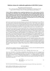
relations. The most notable conceptual neighborhood graphs come from the simple-region relations (Egenhofer and Al-Taha 1992), line-line relations (Reis et al. 2008), region-line and line-region relations (Egenhofer and Mark 1995), and the region-region relations on the sphere (Egenhofer 2005). These conceptual neighborhood graphs provide relevant information for crossing the divides between relations such as disjoint and meet. Conceptual neighborhood graphs are not always consistent, though. There are different concepts of neighborhoods that can be formed and are relevant. For example, there are three neighborhoods for the eight topological region-region relations (Figure 2.1).
(a)
(b)
(c)
Figure 2.1. A-, B-, and C-Neighborhoods of the eight topological region-region relations (Gooday and Cohn, 1994). Each of the neighborhood graphs shows the relationships between relations under a certain deformation (Freksa, 1992). The A-neighborhood (Figure 2.1a) shows the path
23
between objects under the deformations of scaling, rotation, and translation; the Bneighborhood (Figure 2.1b) shows the path between objects under the deformations of shape, size, and orientation (Egenhofer and Al-Taha 1992); and the C-neighborhood (Figure 2.1c) shows the path between objects under isometric deformation. The Aneighborhood is the predominant neighborhood discussed in applications as the types of changes considered have the least dependency on the objects involved in the relations.
2.8 Hamming Distances An important capacity of many data-entry systems is its ability to check for and correct errors. In this light, a measure of distance between two equal-length data entries was developed in 1950 to assist in the error detection and correction process. This distance is known as the Hamming distance (Hamming, 1950). It is computed by comparing each individual symbol between two character strings of equal cardinality. For each difference in corresponding symbols, a value of 1 is assessed. If the symbols are equal, no distance is recorded. The Hamming distance forms a metric space, satisfying the metric properties of identity, symmetry, and the triangle inequality. An example of an application of Hamming distances can be found in contemporary word processors, which notice common-place misspellings that result from mistyping a small number of characters. Levenshtein distances (Levenshtein, 1966) are an extension to the Hamming distance, accounting for added characters, omitted characters, or swapped characters.
24
2.9 Summary Throughout this chapter, models of spatial relations and different concepts for assessing similarities have been addressed. Currently, many of the established sets of spatial relations do not have conceptual neighborhood graphs, results which are necessary for effective spatial inferences. The concept of a Hamming distance has been used to correct and detect errors in word processors and other interfaces, but it may prove to have more functionality when used in different contexts.
25
Chapter 3
AN ADDRESSING SCHEME FOR 9-INTERSECTION RELATIONS
This chapter develops a consistent numerical addressing scheme for 9-intersection matrices (Figure 3.1). To date, 9-intersection relations have been represented either by 3 x 3 matrices of empty and non-empty values, or by uniquely identifying semantic labels, such as disjoint or covers. The intent is to obtain a reference model that allows for numerical inferences of connections between matrices, unlocking the door to cross-type conceptual neighborhood graphs (e.g., linking a line-region conceptual neighborhood graph to the corresponding region-region conceptual neighborhood graph). Definitions and theorems are provided to allow for formal inferences based solely on the address of the matrix, making the visualization and the origin of the matrix purely complementary. Bo
∂B
Ao ∂A A-
Figure 3.1. Structure of the 9-intersection matrix. 26
B-
3.1 Properties of a 9-Intersection Addressing Scheme The 9-intersection matrix is a symbolic representation of binary topological relations between spatial objects considering the objects’ interiors, boundaries, and exteriors. These labels have been primarily in the form of natural-language like terms (as in the case for the eight region-region relations in R2 or the eleven region-region relations on the sphere) in order to simplify memorizing them. For other sets of relations based on the 9-intersection, a sequential numbering of the relevant subset of relations has been a popular choice—for line-line relations (Egenhofer, 1993), for line-region relations (Egenhofer and Mark, 1995), for region-region relations with broad boundaries (Clementini and di Felice, 1996), for topological relations between complex spatial objects (Schneider and Behr 2006), and for broad-boundary line-line relations (Reis et al., 2008). All labeling schemes result in labels that are essentially on a nominal scale (as the sequential ordering exposes no particular meaning among the relations), which prevents a unique and consistent mapping from a label onto the corresponding 9-intersection. Unlike the matrix representation, the nominal labels also lack the support to infer any algebraic properties of the relations (such as symmetry and converseness). As the interest shifts into exploring the entire range of 9-intersection matrices with respect to their pertinence in different settings for different specifications of spatial objects, a consistent globally applicable addressing scheme is required. The desiderata for a consistent labeling scheme are as follows: •
It should be applicable to all 512 empty/non-empty matrices that the 9-intersection distinguishes.
27
•
The mapping (μ) from a 9-intersection matrix onto a topological relation label must be unique so that no two different matrices map onto the same label.
•
There should exist an inverse mapping (μ-1) from a topological relation label onto a 9intersection matrix.
•
The inverse mapping must produce unique 9-intersection matrices (i.e., no matrix inferred from two different labels must be the same).
•
μ-1(μ(9-intersection matrix)) = 9-intersection matrix and μ(μ-1(topological relation label)) = topological relation label.
•
The labels should be such that the relations’ algebraic properties (symmetry, converseness) can be inferred from the labels.
•
The algebraic properties inferred from the labels much be the same as the algebraic properties inferred form their corresponding 9-intersection matrices.
Figure 3.2. The mappings µand µ-1 in relation to their analyses and algebraic properties.
28
Another two constraints put these desiderata into a more constrained framework: •
The mappings are complete if all algebraic properties that can be derived from the 9interesection matrices can be derived from the topological-relation labels as well.
•
The mapping are consistent if all algebraic properties derived from the 9-interesection matrices are the identical to those derived from the topological-relation labels.
3.2 Binary Numbers and Connectedness Each cell in the 9-intersection matrix can have one of two values: 0 representing an empty intersection and 1 representing a non-empty intersection between the specified topological parts of A and B. It is desirable to have a single number associated with each matrix that would uniquely identify it. Since each cell has a value of either 0 or 1, it is possible to produce a binary coding of this matrix by appending the 0s and 1s into a binary digit string in some explicit order and then converting this binary digit string into its corresponding decimal form. To obtain such a framework, we must start with defining the alphabet of our formal language. This alphabet is structured based on the notion of binary notations. A similar method has been attempted for 3D relations (Jun and Xiaolin, 2008), but the full powers of which have not been explored.
Definition 3.2.1. The binary notation βK of an integer K is composed by successively
dividing K by 2 and recording the remainder from right to left.
To exhibit Definition 3.2.1, the binary notation of 44 (Table 3.1) is considered. 29
Table 3.1. Binary decomposition of 44, yielding 101100 by concatenation of remainders Number
Quotient (Number/2)
Remainder
44
22
0
22
11
0
11
5
1
5
2
1
2
1
0
1
0
1
The binary notation of an integer is order-dependent in just the same way as the decimal notation of an integer is order-dependent. Instead of multiplying each digit by the corresponding power of 10 from right to left and then adding them together to produce the number, we multiply each digit by the corresponding power of 2 from right to left and then adding them together.
Theorem 3.2.2.
n −1
∑2
i
= 2n − 1
i =0
Theorem 3.2.2 essentially states that no power of 2 can be expressed explicitly as the sum of distinct powers of 2. The consequence of Theorem 3.2.2 allows for the assertion that the binary notation of an integer K is unique. Since βK is unique for every integer K, we have a viable alphabet for our formal language through the concept of binary notations. With this assertion in place, we now affix a labeling to the class of 9intersection matrices. We restrict the domain of interest. Since the consideration is the 9-
30
intersection matrix from Figure 3.1, the domain is restricted to capture only enough labels for a one-to-one and onto correspondence, thus ensuring the existence of an inverse function µ-1. All of these concepts would apply for any domain set, but for ease of statement and the existence of an inverse function, we choose to restrict the domain.
Definition 3.2.3. A label for a 9-intersection matrix, denoted as λ, is a member of the set
{0, 1, 2, … , 511}. The set of all such labels λ is denoted as Λ.
With a label set in place, the next step is to define the notion of connection. In order to produce conceptual neighborhood graphs of immediate neighbor relations, it is critical to identify methods that link the addresses that are formed under this alphabet of binary notation. This goal results in studying the subset connectivity of these ordered binary notation sets.
Definition 3.2.4. λ1 ∈ Λ is connected from above to λ2 ∈ Λ if λ1 − λ2 = 2m and the mth
member of β λ1 = 1. λ1 ∈ Λ is connected from below to λ2 ∈ Λ if λ2 − λ1 = 2m and the
mth member of β λ2 = 1. If either of these relations holds between λ1 and λ2 , λ1 and λ2 are said to be connected.
This definition of connected from above implies that λ1 is not connected from above to itself and that λ1 > λ2 . Likewise, connected from below implies that λ1 is not connected to itself and λ1 < λ2 . An example of two numbers that are connected from
31
above is λ1 = 63 and λ2 = 31. Converting them to 9-digit binary notations, 63 = {0,0,0,1,1,1,1,1,1} while 31 = {0,0,0,0,1,1,1,1,1} where m = 5. An example of two numbers connected from below is λ1 = 14 and λ2 = 15. Using their 9-digit binary notations, 14 = {0,0,0,0,0,1,1,1,0} while 15 = {0,0,0,0,0,1,1,1,1}, where m = 0. The visualization of these binary notations shows a specific result that is presented as Theorem 3.2.5.
Theorem 3.2.5. If λ1 and λ2 are connected, then for exactly one m, the mth member of their
binary representations differ for exactly one m.
Proof: If λ1 and λ2 are connected, then they are either connected from above or connected
from below. If they are connected from above, λ1 – λ2 = 2m, and mth member of β λ1 = 1. Since 2m is a power of 2, changing this 1 to a 0 converts λ1 into λ2 directly. If they are
connected from below, λ2 – λ1 = 2m, and mth member of β λ2 = 1. Since 2m is a power of 2, changing this 1 to a 0 converts λ2 into λ1 directly.
■
By Theorem 3.2.5, neighboring labels have been defined by having binary notations that differ in exactly one member, namely the mth members of each β. The mth member of a binary notation is the mth power of 2 considered in the binary notation (which reads right-to-left). This definition of connection represents a Hamming distance (Hamming, 1950) between the binary representations of the labels of exactly 1. We have established connectivity by a means of the binary notation of the subsets via the Hamming distance calculation. This relationship can now be translated back into a 32
numerical form that does not fulfill the same Hamming distance qualities. While this step of conversion is not necessary, it provides the ability for a shorter notation and more generalized form for non-mathematical users.
Theorem 3.2.6. Let λ ∈ Λ be arbitrary. Let J = 2n such that J ≤ λ and 2J > λ. Let I = 2m
such that J < I < 512. Label λ is connected to label λ + I for all I.
Proof: Since λ < I, βλ(m) = 0. Since I is a power of 2, A must be connected from below to λ
+ I because (λ + I) – λ = 2m. Thus λ is connected to λ + I.
■
Theorem 3.2.7. Let λ ∈ Λ be arbitrary. Let J = 2m such that J ≤ λ and 2J > λ. Label λ is
connected to label λ – J.
Proof: Since λ – (λ – J) = J, λ is connected from above to λ – J (Definition 4.1.4). Thus λ is
connected to λ – J.
■
Theorem 3.2.8. Let λ ∈ Λ be arbitrary. Let J = 2n such that J ≤ λ and 2J > λ. Let I = λ – J
and G be connected from below to I. Let F = J + G. Then label λ is connected to label F.
Proof: Since I = λ – J, λ – I = J algebraically. Because J is a power of 2, λ is connected
from above to I. Since G is connected from below to I, I – G = 2m. From Theorem 4.1.2, It is known that both λ and F are unique sums of powers of 2. To prove the theorem, it must be shown that the mth member of Bλ = 1 and that λ – F = 2m. Since I – G = 2m, the mth
33
member of BI = 1. I is connected to λ and λ > I, so the mth member of λ is also 1. Because
λ – F = I – G = 2m, the mth member of F must also be 0.
■
Now that connectivity has been established, it is possible to move on to special matrix relations.
3.3 Binary Numbers for 9-Intersection Matrices This section presents the application of the theorems and definitions presented in Section 3.2. The addressing scheme is concretely assigned, allowing for the definition of a
negation of a topological relation and a converse of a topological relation. Using the connection theorems from Section 3.2, we construct a conceptual neighborhood graph for the power set of the 9-intersection matrix. The negation of a matrix represents the matrix with a Hamming distance of exactly 9. This statement implies that each entry in the matrix must be reversed. From this construction, we derive Theorem 3.3.1.
Theorem 3.3.1. The negation η(λ) has label 511 – λ.
Proof: If we add the binary notations of λ and η(λ), we obtain 111111111. Converting this
binary number to decimal notation, we obtain 511. Thus η(λ) = 511 – λ.
■
The next result of importance is the converse relation matrix, which transposes two spatial objects A and B. The effect upon the 9-intersection matrix can be seen in Figure 34
3.3, where cells of the same shading have the same values in both the matrix and its converse.
Bo
∂B
B-
Ao
a
b
C
∂A
d
e
A-
g
h
Bo
∂B
B-
Ao
a
d
g
F
∂A
b
e
h
I
A-
c
f
i
(b)
(a)
Figure 3.3. Comparison of 9-intersection matrices: (a) a 9-intersection matrix and (b) its converse. Cells with identical letters represent identical information.
Part of imposing a numeric addressing system is to have a predictable converse based solely on the label of the original matrix (Section 3.1). There are many ways for a function to be predictable. The two major routes for this goal are to have a specific algebraic equation that models the entire space or to have a repeating periodic sequence that represents the process explicitly. Considering the structure that is apparent in the converse of any matrix (including a 9-intersection matrix), a periodic sequence is far more likely to occur. Three cells in the matrix—those on the main diagonal—maintain the same values in both the matrix and the matrix of the converse relation. This result is intuitively periodic if the cells are associated with the correct powers of 2. This instance is the first time where the address of the particular cell matters in the theorem set. In defining functions, a smaller period is conceptually easier to understand than a larger period, so the smallest binary units are used to construct the cells affected by
35
the converse relation. This choice minimizes the period. If the cell addresses are chosen in a proper way, a predictable periodic function may result. A 1 x 9 slot array, each slot numbered ascending with an integer from [0,8], is used to maintain the positioning.
Definition 3.3.2. The converse additive, denoted by Γ(λ), is λ – the label of its converse.
The diagonal cells of the 9-intersection matrix are placed arbitrarily in the 7th, 8th, and 9th slots of the array. The ordering selected for these three is ultimately inconsequential so long as consistency is maintained, because the diagonal is not affected under the converse operation. We select exterior-exterior to occupy slot 7, boundaryboundary to occupy slot 8, and interior-interior slot 9. Using this configuration, the smallest binary powers are reserved for the cells that are affected by the converse operation.
Theorem 3.3.3. Γ(λ) is a periodic function with a maximum period length of 64.
Proof: Because the diagonal members of the matrix remain constant under the converse
relation, the diagonal measures are present in both the original matrix and the converse relation. Let R be the set of diagonal entry in the matrix with label λ. Let S be the label of the matrix only containing R. Then λ = S + Z with 0 ≤ Z ≤ 63. Let T be the label of the converse of λ. T = λ – Γ(λ) = S + Z – Γ(λ). The sum S can be cancelled without affecting the function as it is in common with both T and λ. Thus Γ(λ) is a periodic function. Since Z can take on 64 possible values, the function has a maximum period length of 64.
36
■
Selecting values that differ by one across the diagonal (i.e., boundary-interior and interior-boundary) makes the function most predictable as there is a systematic difference between cells transposed under converse. Using the conventions of this one-difference and the largest values being placed on the diagonal, all cells can now be addressed with their respective placeholders. Figure 3.4 shows the positioning in the slot array by placing the number in the cell of the 9-intersection matrix. The values of Γ(λ) are computed for the first period and are given numerically in Table 3.2 and graphically in Figure 3.5.
Bo
∂B
B-
Ao
8
2
0
∂A
3
7
4
A-
1
5
6
Figure 3.4. 9-Intersection matrix imposed with the cell positions within the slot array.
37
Table 3.2. λ (mod 64) related to Γ(λ)
λ Γ(λ)
λ Γ(λ)
λ Γ(λ)
λ Γ(λ)
0 0
16 -16
32 16
48 0
1 -1
17 -17
33 15
49 -1
2 1
18 -15
34 17
50 1
3 0
19 -16
35 16
51 0
4 -4
20 -20
36 12
52 -4
5 -5
21 -21
37 11
53 -5
6 -3
22 -19
38 13
54 -3
7 -4
23 -20
39 12
55 -4
8 4
24 -12
40 20
56 4
9 3
25 -13
41 19
57 3
10 5
26 -11
42 21
58 5
11 4
27 -12
43 20
59 4
12 0
28 -16
44 16
60 0
13 -1
29 -17
45 15
61 -1
14 1
30 -15
46 17
62 1
15 0
31 -16
47 16
63 0
38
Γ(λ) mod 64
Figure 3.5. Graph of the first period of Γ(λ).
Now consider the region-region relations. To exhibit the functionality of this numbering scheme, the region relations have their matrices, converse matrices, and connected matrices identified via the constructs of this chapter. Table 3.3 represents the values of λ corresponding to region-region relations. These values are taken and placed through the theorems and definitions presented to establish the connections and converse matrices.
39
Table 3.3. Binary codings of the eight region-region relations
disjoint
115
meet
243
overlap
511
equal
448
contains
341
covers
469
inside
362
coveredBy
490
The accuracy of the theorems can be checked by passing through the connections from the A-neighborhood of the region-region relations (Egenhofer and Al-Taha, 1992). In this conceptual neighborhood graph (Figure 2.1a), disjoint connects to meet, meet connects to overlap, overlap connects to covers, overlap connects to coveredBy, covers connects to
contains, covers connects to equal, coveredBy connects to equal, and coveredBy connects to inside. The theory should preserve all of these connections to be accurate. Each of these relations is evaluated one by one. The results of this evaluation are presented as Table 3.4.
40
Table 3.4. A-Neighborhood connections evaluated through connection theorems
Label of Relation 1
Label of Relation 2
Relation 1
Connected by Connection
Relation 2
Theorem 4.2.4
disjoint
115
meet
243
direct
below
meet
243
overlap
511
indirect
through 251 (below) and 255 (below)
overlap
511
covers
469
indirect
through 479 (above) and 471 (above)
overlap
511
coveredBy
490
indirect
through 495 (above) and 491 (above)
covers
469
contains
341
direct
above
covers
469
equal
448
indirect
through 468 (above) and 452 (above)
coveredBy
490
inside
362
direct
above
coveredBy
490
equal
448
indirect
through 482 (above) and 450 (above)
These results show that a single direction linkage exists for all eight region-region relations. It also shows, however, that this linkage sometimes has a Hamming distance > 1. This result has happened because a subset of the power set of 9-intersection matrices was considered. Since only eight relations are realizable between two simple regions and there are only matrices that contain 3, 5, 6, and 9 non-empty intersections, it impossible for these relations to be directly connected under this method of defining connection.
41
3.4 Graph Generation of the 9-Intersection Addressing Scheme Since the label space Λ is larger than the set of region-region relations, it is often the case that for a particular label there does not exist a corresponding region-region relation. For example, the label 411 does not exist in the set of region-region relations, but the label 490 exists (for coveredBy). Thus we are now considering a subset of all the relations for which we need to find connectivity. It then makes sense that connection in a subset should not necessarily be restrictively linked to a Hamming distance of 1. Conceptual neighborhood graphs need the capacity to link all member relations, not just those that happen to have a Hamming distance of 1. This requires the development of subset connectivity. Subset connectivity refers to the aggregation of the smaller connections that exist between different relational labels. It becomes the vehicle for linking such relations as
overlap and meet, which have a Hamming distance of 3. To define this notion of subset connectivity, we must first have a graph of all the connections present in the label set Λ. From this graph, we then define the concept of path and the concept of shortest path.
Definition 3.4.1. λ is represented by a node in the neighborhood graph of matrices.
Definition 3.4.2. Let λ1 and λ2 be labels such that λ1 is connected to λ2 . The segment
[ λ1 , λ2 ] is an edge in the graph of matrix relations.
Definitions 3.4.1 and 3.4.2 lead to a graph of all relations and their connected labels.
42
Definition 3.4.3. Let G be a graph with nodes connected by edges. A path P is an ordered
sequence of distinct connected nodes linked by distinct connected edges of G.
An example path extends from the empty relation (with all empty entries) to
overlap (all non-empty entries). This path requires iteratively adding each cell to the matrix; therefore, the path of labels {0, 1, 3, 7, 15, 31, 63, 127, 255, 511} is one of many possible paths from the empty relation to overlap.
Definition 3.4.4. Define P as the shortest path from λ1 to λ2 if the Hamming distance
between λ1 and λ2 is minimized, considering all possible paths from λ1 to λ2 .
Definition 3.4.5. Let λ1 and λ2 be labels and X be a subset containing λ1 and λ2 . λ1 is connected to λ2 in X if all shortest paths from λ1 to λ2 pass through at least one label from
the complement of the subset X or if λ1 is connected to λ2 via definition.
3.4.1 Region-Region Relations Using Definitions 3.4.3 through 3.4.5, the connections exhibited in the eight region-region relations subset are established (Table 3.5). This table produces the A-neighborhood of a conceptual neighborhood graph.
43
Table 3.5. Connected labels in the region-region subset
disjoint (115)
meet (243)
meet (243)
disjoint (115), overlap (511)
overlap (511)
meet (243), covers (469), coveredBy (490)
equal (448)
covers (469), coveredBy (490)
contains (341)
covers (469)
covers (469)
contains (341), equal (448), overlap (511)
inside (362)
coveredBy (490)
coveredBy (490)
inside (362), equal (448), overlap (511)
The negated relations for the eight region-region relations (Table 3.6) are absent from the region-region relations subset. This omission makes perfect sense as the objects in each relation must have every opposite value in the cell. If this were possible, then there must be a relation which does not contain the exterior-exterior intersection. Negation of these relations thus implies that none of the objects forming the relations may have coincident exteriors. If the relations cannot have coincident exteriors, they either have no exteriors at all or the interior and boundary of one set exhaust the exterior of the other set. Either way, these relations do not exist in the defined region-region relations.
44
Table 3.6. Labels of the eight region-region relation negations
disjoint (115)
396
meet (243)
268
overlap (511)
0
equal (448)
63
contains (341)
170
covers (469)
42
inside (362)
149
coveredBy (490)
21
The converse function should identify symmetric relations as their own converse. Those relations that are not symmetric should return a relation that is within the subset itself (as the candidate relation would be viable). Table 3.7 shows the converse relations of the eight region-region relations, confirming that the converse is in fact a member of the subset of region-region relations and furthermore that the arithmetic used to generate the converse produces identical results to considering the converse configuration and calculating its label. The contents of this table are produced by taking the label for the relation, dividing it by 64 and considering its remainder, using the value from Table 3.2 associated with this remainder, and then calculating the converse.
45
Table 3.7. Converse in the region-region subset
Relation and label
Remainder of label (mod 64)
Converse label and relation
disjoint (115)
51
115 – 0 = 115 – disjoint
meet (243)
51
243 – 0 = 243 – meet
overlap (511)
63
511 – 0 = 511 – overlap
equal (448)
0
448 – 0 = 448 – equal
contains (341)
21
341 + 21 = 362 – inside
covers (469)
21
469 + 21 = 490 – coveredBy
inside (362)
42
362 – 21 = 341 – contains
coveredBy (490)
42
490 – 21 = 469 – covers
3.4.2 Line-Region Relations and Region-Line Relations The simple line-region relations (Figure 3.6) are now used with the converse rules to derive the simple region-line relations (Table 3.8), further confirming the validity of such a mathematical numbering scheme.
46
Figure 3.6. The 19 line-region relations identified with the 9-intersection (Egenhofer and Mark, 1995).
47
Table 3.8. Converses of the line-region relations
Relation
Remainder (mod 64)
Converse Relation
383
63
383
367
47
351
366
46
349
362
42
341
495
47
479
494
46
477
490
42
469
375
55
379
503
55
507
487
39
475
486
38
473
482
34
465
119
55
123
247
55
251
231
39
219
230
38
217
115
51
115
243
51
243
227
35
211
48
3.4.3 Graph of All Labels Using Theorems 3.2.6 and 3.2.8 and the rules defined in Definitions 3.4.1 and 3.4.2, the graph of Λ can be generated. In order to generate the graph for all λ∈Λ, it is necessary to add two more concepts (Definitions 3.4.6 and 3.4.7).
Definition 3.4.6. The subset adjacency matrix C↓ is the matrix formed by the following
rule: if λ1 is connected from below to λ2 , then C↓ [ λ1 , λ2 ]=1, else C↓[ λ1 , λ2 ]=0.
Definition 3.4.7. The superset adjacency matrix C↑ is the matrix formed by the
following rule: if λ1 is connected from above to λ2 , then C↑[ λ1 , λ2 ]=1, else C↑[ λ1 , λ2 ]=0.
Using these adjacency matrices, the graph G can be encapsulated for the first time in a realizable form. Using either of these adjacency matrices, G can be compiled by adding an edge from λ1 to λ2 wherever the value in their ordered pair is 1 (Figure 3.7).
3.5 Summary and Assessment Through the course of Chapter 3, we derive a syntactical label set to replace the semanticbased language labels for the 9-intersection matrices. These labels form a set Λ and provide a naming power for the sets of relations found in Chapter 2. The label set has many mathematical properties and relationships that can be utilized to assist in 9-intersection pursuits. Negations, converses, and a notion of connectivity are defined strictly through these syntactical labels. Theorem 3.2.5 asserts
49
that connectivity is based in the construction of Hamming distances (Hamming, 1950). We also showed that the mathematical constructions of the label set produce desired results (identical for the eight region-region relations) and that a subset of relations may not be connected strictly by Hamming distance 1. Subset connectivity is thus defined to answer this issue. The aforementioned graph of the set Λ is such that any particular label must be connected to nine other labels. It is impossible for this graph to be planar by Kuratowski’s Theorem (Adams and Franzosa, 2008). Utilizing the aggregated paths from the nodes 152, 164, and 448 to 0, 128, and 508, the graph of the set Λ contains a subgraph homeomorphic to K3,3. For this reason, Figure 3.7 appears in a fairly confusing form. The alignment of Figure 3.7 is such that all nodes on the same level have the same number of non-empty intersections. The top-most level has 9 non-empty intersections, while the bottom-most level has 0 non-empty intersections.
50
51
Figure 3.7. Graph of the nodes and connections of Λ.
Chapter 4
ANALYSIS OF THE GRAPH WITH REGARD TO SUBSETS OF 9-INTERSECTION RELATIONS
In this chapter, the graph of Λ (Figure 3.7) is utilized to derive conceptual neighborhood graphs of 9-intersection relations for several sets of spatial relations. Systematic structures and patterns are assessed for each graph. With the plotting interface of the statistical and graphing software R 2.8.0, the graph can be modified to exhibit the connections between the subset graphs. In general, the graphs of the relations are not necessarily planar, so the elegancy of the eight region-region relations is not a reasonable expectation.
4.1 Eight Region-Region Relations (Egenhofer and Franzosa, 1991) In giving examples for Chapter 3, the labels representing these relations have been computed and presented in the body of this work. Since some of the eight region-region relations are not connected directly in the graph, extra matrices are needed to fill the gaps between pairs of relations with a Hamming distance > 1. The matrices that fill the gaps are not a part of this subset of relations. Figure 4.1 shows the graph of this subset with
52
connections exposed. Using connected in the subset (Definition 3.4.5) and the shortest
path (Definition 3.4.4), we have created the A-neighborhood for the set of relations
4.2 Spherical Relations (Egenhofer, 2005) The eleven spherical relations show the exact same patterns as the eight planar regionregion relations. The difference, however, is that another leg is added to the graph, representing the exhaustion of space with the addition of the relations entwined, embrace, and attach. The A-neighborhood of this relation subset is also identified through this basis generator. Figure 4.2 shows the graph of this subset with its connections exposed.
4.3 Li Relations (Li, 2006) Figures 4.1 and 4.2 demonstrate that not all subsets of topological relations are directly connected in the graph of Λ. The Li relations provide some meaningful insight into the structure of the region-region graph and the spherical relations graph, specifically about the transformation between more distant neighbors such as equal to coveredBy or overlap to meet. There are six possible paths from each pair of neighbors with a Hamming distance of 3. Knowledge of these intermediary relations limits the number of paths that are actually possible. The Li relations are fully connected. None of the realizable relations are offset from any of the others (i.e., every label connects directly to another one in the subset). The Li relations are of binary complex regions. Each of these relations has a different 9intersection matrix and label, but the objects also may have holes and separations as well. Of the two types of situations presented as examples of Hamming distance 3, the 53
54
Figure 4.1. Graph of the eight region-region relations subset, featuring jumps from equal and overlap.
55
Figure 4.2. Graph of the spherical relations subset, also exhibiting jumps for equal, overlap, and attach.
easiest conceptual progression to understand is from overlap to meet. This transference is analogous to the transference that occurs in overlap to any of the other similar jumps in the graph (e.g., covers). Throughout Section 4.3, pink objects are region A, blue objects are region B, and a coincidence of A and B is purple.
4.3.1 overlap (511) to meet (243) Theorems 3.2.4 and 3.4.3 generate six possible paths from overlap (511) to meet (243): {511, 507, 499, 243}, {511, 507, 251, 243}, {511, 503, 499, 243}, {511, 503, 247, 243}, {511, 255, 247, 243}, and {511, 255, 251, 243}. Only 499 (PO11), 503 (PO15), and 507 (PO13) are among the Li relations, however, leaving only {511, 507, 499, 243} and {511, 503, 499, 243} for consideration. A graphic representation of the transference between
overlap and meet is shown in Figure 4.3.
511 (a) a
243 (e) e
507 (d) d (b) b
(c) c 499
511
243
503 Figure 4.3. Transference from overlap to meet: (a) induce a separation upon both regions, (b) collapse the overlapping component of one object into the other object, yielding 503 or 507, (c) reduce the opposite overlapping component to the same size, yielding 499, (d)
56
slide one of the equal components such that they share only a portion of their boundary, and (e) delete the created separation.
A certain sequence of transformations must occur to transfer between object relations as in Figure 4.3. First, unless the regions are already separated, they must each endure a separation such that one piece of one object remains covering one piece of the other object while the other pieces are disjoint. Second, the covering object must be shrunken down until it equals the covered piece. Third, the objects must move until just the boundaries are in contact. Merging is not necessary to obtain relation 243, but for the sake of completeness and compatibility with the initial configuration, we display meet as two regular regions, implying that a merge has occurred.
4.3.2 overlap (511) to entwined (399) For the transference from overlap (511) to entwined (399), six paths are possible: {511, 495, 463, 399}, {511, 495, 431, 399}, {511, 479, 463, 399}, {511, 479, 415, 399}, {511, 447, 431, 399}, and {511, 447, 415, 399}. Of the matrices in these paths, only three are possible: 463 (PO16), 479 (PO17), and 495 (PO18), which reduces the potential paths to {511, 495, 463, 399} and {511, 479, 463, 399}. Figure 4.4 shows the transference from
overlap to entwined.
57
511
399
479
(a)
(e) (d) (c)
(b)
463
511
399
495 Figure 4.4. Transference from overlap to entwined: (a) create an equal hole in both objects in the overlapping region, (b) drag one object to exhaust its external space, (c) drag the other object to exhaust its external space, (d) fill the hole with one object, and (e) fill the hole with the other object.
Again, a certain sequence of transformations must occur. First we must create a hole in both objects contained in the intersection. Second, one object must be extended such that its boundary is removed from the exterior. Third, we must extend the other object in a similar way. Finally, we fill in the hole created in the first step to produce the relation
entwined. Since overlap and entwined are both symmetric, reversing the colorations moves along the bottom of the figure.
4.3.3 overlap (511) to coveredBy (490) and covers (369) For the transference from overlap (511) to coveredBy (490), there are again six potential paths: {511, 510, 506, 490}, {511, 510, 494, 490}, {511, 507, 506, 490}, {511, 507, 491,
58
490}, {511, 495, 494, 490}, and {511, 495, 491, 490}. Along these potential paths, only three matrices are realizable: 491 (PO12), 495 (PO17), and 507 (PO13), which leaves us with two potential paths: {511, 507, 491, 490} and {511, 495, 491, 490}. Figure 4.5 shows a pictorial representation of the transference between these two relations. 511
490
507
(a)
(e) (d)
(b)
(c) 491
511
490
495 Figure 4.5. Transference from overlap to coveredBy (and conversely covers): (a) induce a separation in one object (shown for both for simplicity), (b) shrink one overlapping region down so that it is covered by the other, (c) engulf the boundary of the first object, (d) exhaust the area of the first object with the second object, and (e) merge the separated first object.
We sever the two regions such that one piece of one region sits inside the part of another on its boundary, and the other two pieces are disjoint. The second step takes the second region and engulfs the pieces of the first object while not entering them. The final
59
step engulfs those parts of the first object that were in the exterior of the second object, yielding coveredBy. This is also conversely true for covers by reversing the colors, reflecting as intermediary relations 471 (PO14), 479 (PO18), and 503 (PO15).
4.3.4 Comparisons In all of these scenarios (Figures 4.3–4.5), the regions of the intermediary relation must have holes or separations, while the beginning and ending relations are also realizable for region without holes or separations. This distinction is the reason for the gaps in both Figures 4.1 and 4.2 that had to be filled by intermediary relations. Certain patterns exist in the paths that are realizable in these transferences. To go down the superset adjacency matrix (overlap to meet) requires the removal of the boundary intersections, followed by the interior-interior intersection. This same pattern of removing boundary intersections first happens for the other three legs of the graph as well. Similarly, moving up the subset adjacency matrix (meet to overlap) requires adding the two-dimensional intersection (e.g., interior-interior), followed by the addition of the boundary intersections.
4.3.5 equal (448) to coveredBy (490) The transference between equal (448) and coveredBy (490) is a little different, however. There still exist six possible paths between the two relations: {448, 456, 458, 490}, {448, 456, 488, 490}, {448, 450, 458, 490}, {448, 450, 482, 490}, {448, 480, 482, 490}, and {448, 480, 488, 490}. Coincidentally three of these relations can be found in Li’s method:
60
450 (TPP1), 458 (TPP3), and 482 (TPP2), leaving exactly two paths: {448, 450, 458, 490} and {448, 450, 482, 490}. Where this sequence differs from the previous examples is that Li alludes to the existence of exotic regions (i.e., regions that share the entire boundary yet are not complementary or equal). In this case, we are referring to label 450. These types of regions do not exist in our realizable world in a connected form, because they are produced through infinite sequences. They do exist in our world, however, in a separated form through looking at some complex dynamic systems. An image of such a separated exotic region can be created by taking spherical Christmas ornaments, aligning them in a tetrahedral formation, covering up sources of light from all but one side, and then shining a light inside the configuration from the remaining side. The reflective powers of the ornaments will produce a highly complex fractal, which demonstrates the exotic regions. Figure 4.6 shows a picture of the formation of a system of connected Wada regions.
Figure 4.6. First iteration of the Lakes of Wada procedure for four lakes.
61
The Wada relations are named as follows: Wada coveredBy is represented by regions A = {blue} and B = {blue, red}; Wada covers is represented by regions A = {blue, red} and B = {blue}; Wada meet is represented by regions A = {green} and B = {yellow};
Wada entwined is represented by regions A = {blue, red} and B = {red, yellow, green}; and Wada overlap is represented as A = {blue, red} and B = {red, green}. Li makes the claim that the relations are all realizable with only 3 regions, however his realizations of M6 and M7 (Li, 2006) both entirely exhaust the space, making them both equivalent, not distinct, matrices. With this imagery in hand, Figure 4.7 shows the process to convert from
equal to coveredBy.
482
448
450
490 458
Figure 4.7. Transference from equal to coveredBy (and conversely covers by switching blue to pink).
A certain sequence of topological changes must occur: first, we must go from a region A which is equal to another region B, maintain the entirety of common boundary while growing region B. This step yields Wada coveredBy. From here, we must peel away part of the common boundary by adding to one boundary but not the other (which can be done by adding a second piece altogether or inserting a hole in one). Finally coveredBy is obtained by merging region B or collapsing region A. 62
4.3.6 Similarities between the Transferences from overlap to coveredBy and from equal to coveredBy In both of the title cases, exactly two paths exist and the sequence of adding to the matrices is the exact same. To ascend the subset adjacency matrix (and thus the graph), one must first add the corner entry (i.e. interior-interior), then add one of two boundary entry, and then add the other boundary entry. The Wada relations help us to see exactly how the transformations from equal and attach actually manifest themselves. The lack of Wada relations causes a gap in the region-region relations that is seemingly irreconcilable. This method of computing connections provides concrete evidence for why the Wada regions must exist in object space. Knowledge of the surrounding relations actually helps to pinpoint what the configuration would look like. Figure 4.8 shows the graph of the Li relations. Unfortunately the Li relations are incomplete in that they allow for exhaustion of space by two objects, but do not allow one object to accomplish this feat, allowing for more spatial relations (though trivial they may be) to exist.
4.4 Schneider and Behr (2006) Region-Region Relations The Schneider/Behr region-region relations are a subset of the Li relations. Their subgraph is disconnected (Figure 4.9) because of the missing exotic regions and complementary regions. This omission is not subtle in that it places a separation in the graph from equal up to the intermediary relations leading to covers and coveredBy.
63
64
Figure 4.8. Graph of the Li region-region relations subset.
65
Figure 4.9. Graph of the Schneider/Behr region-region relations.
4.5 Simple Line-Region Relations (Egenhofer and Mark, 1995) The line-region relations are simple in that they deal with a continuous line segment and a regular region. This section also considers the converse of these relations, namely the simple region-line relations. The existing conceptual neighborhood graph for these relations (Figure 3.6) is replicated exactly through this basis generator. This set of relations gives further validity of the power and applicability of the labeling process. The derived conceptual neighborhood graphs for the line-region and region-line relations are shown in Figures 4.10 and 4.11, respectively.
4.6 Complex Line-Region Relations (Schneider and Behr 2006) The complex line-region relations proposed by Schneider and Behr (2006) show the relations between a complex line and a complex region. Complex regions have separations or holes, while complex lines have multiple extremities (whether forked or separated) or no extremities, leading to cycles. There are 82 possible relations under their method. These relations do not account for the ability to exhaust a space by one or more objects. Further consideration needs to be given in this area to complete the set. The complex line-region relations form a connected set in the graph (Figure 4.12), and so do the converse relations, the region-line relations (Figure 4.13).
66
67
Figure 4.10. Graph of the simple line-region relations subset.
68
Figure 4.11. Graph of the simple region-line relations subset.
69
Figure 4.12. Graph of the Schneider/Behr line-region relations subset.
70
Figure 4.13. Graph of the Schneider/Behr region-line relations subset.
4.7 Line-Line Relations (Egenhofer 1993; Reis et al. 2008, Schneider and Behr 2006) The line-line relations come in two forms: simple lines and complex lines. Thirty-three relations have been accounted for between two simple lines, while 57 have been found for two lines with multiple boundary points. If one also allows for cycles (i.e., lines with no boundary) and separations, a total of 82 relations with complex lines apply. The line-line relations give us the first opportunity to realize a matrix with only two non-empty intersections as the ability to have a cycle comes into play. A cycle has no endpoints, therefore it has no boundary in algebraic topology. Everything is either in the interior or the exterior. The line-line relations provide a disconnected and also incomplete neighborhood graph through the basis generator. For the first time, a 9-intersection matrix with five nonempty intersections can lead directly to another 9-intersection matrix with five non-empty intersections in one single step. Given the definition of connection in the context of this thesis, our basis generator cannot capture this transition for the A-neighborhood. This failure in the method might have something to do with the co-dimension of the space and the objects. Since the objects in this case have a degree of freedom that a region would not have, they have additional flexibility. The conceptual neighborhood graphs of the above-mentioned 33, 57, and 82 relations are presented as Figures 4.14, 4.15, and 4.16, respectively. The 82 Schneider relations remain connected, however. These graphs complete Chapter 4 of the thesis. With these graphs, we move further down the line into what the graphs might suggest about relationships across graph subsets.
71
72
Figure 4.14. Graph of the 33 simple line-line relations showing a separation at equal.
73
Figure 4.15. Graph of the 57 complex line-line relations, showing a separation at equal.
74
Figure 4.16. Connected graph of the 82 Schneider/Behr line-line relations.
4.8 Summary and Assessment Although the basis generator is capable of generating an A-neighborhood when at least one object is in co-dimension 0, it says nothing about whether or not the generated neighborhood reflects the only paths that exist in the set of relations. An example of this point is the move from equal to covers. These two relations need not endure the problematic topological deformations of separation and hole-formation to get from one to another, as both can be deformed to each other through expansion and contraction. This connection scheme has a different meaning than typical connection in a conceptual neighborhood graph that is not at first easy to understand, but does make some sense. Being connected in Λ has to do with the differences in the matrix representations. Object relations with the same matrix are equivalent under the matrix only. This notion of equivalence does not imply the topological equivalence of these objects. Connection for our purposes means that there exists at least one member with that particular label that can be deformed using A-neighborhood methods that will produce the connected label. The epitomes of this occurrence are the Wada relations. Though it is generically unnecessary to have these intermediary relations for any practical purposes, there are times when the Wada regions are needed to complete the transitions between two relations conceptually. Similarly separated regions like those used to exhibit the transition from overlap to meet allow us to explore relations for regions other than simple discs. To exhibit these equivalences under the matrices, we have used transformations that may not necessarily reflect topologically equivalent objects. This usage is meant to demonstrate that not all members of a matrix equivalence class are topologically equivalent, demonstrating that the 9-intersection still has some information that it masks away under its premises. 75
Chapter 5
TRANSFORMING RELATIONS ACROSS DIMENSIONS
This chapter provides a framework for linking relations across dimensional frameworks (e.g., line-line relations in R2 to region-region relations in R2). The 9-intersection matrix and the graph of its labels provide a means for connecting the conceptual neighborhood graphs across the relations through the increase or decrease of dimension. This chapter identifies relations under Schneider and Behr’s identification procedure that may lead to link points which will one day combine them into a single conceptual neighborhood graph. Such a conceptual neighborhood graph would make it possible to relate any combination of relations between two objects in R2.
5.1 A Generalized Framework for Graph Connection Through analysis of the Schneider and Behr relations, there are 100 distinct labels that exist in some capacity in R2. Considering the total number of relations identified between objects, however, that number soars to 248 relations between any two spatial objects in R2. Therefore, on average, each distinct label is found in 2.48 of Schneider and Behr’s relational classes. Though the labels themselves are distinct, one label can represent 76
numerous different relations. Table 5.1 shows a frequency distribution of the distinctness of the labels. Table 5.1. Frequency of labels in Schneider/Behr relations
Frequency
Number of Labels
0
411
1
28
2
19
3
30
4
23
It is important to establish where the distinct relations are located in the graph, as these relations represent the problems that complicate inference and similarities across relational classes. All of the 28 distinct labels are located in the relational classes line-line, line-region, and region-line. Eighteen (64.3%) of these relations—79, 95, 111, 127, 195, 199, 203, 207, 215, 235, 239, 255, 325, 330, 449, 450, and 451—are from the line-line class of relations. Five are in the line-region class (230, 334, 366, 486, and 494); another five are in the region-line class (217, 333, 349, 473, and 477); and four of the line-line relations in this grouping (195, 449, 450, and 451) are also represented as exotic regionregion relations in Li’s work. To establish a framework, one must define how the change between relational classes would happen. There are nine different relational classes in R2: point to point, point to line, point to region, line to point, line to line, line to region, region to point, region to line, and region to region. The most logical construction for dimensional changes in objects is on the basis of dimension similarity (i.e., a point must become a line before it
77
becomes a region). An example of this construction is starting with a single point, extending the single point into a single line (containing an infinite number of points), and then finally adding width to the line to create a region (containing an infinite number of lines). If the relational classes are neighbored based on this philosophy, the lattice shown in Figure 5.1 results. This selection for alignment is far from arbitrary. It is conceptually understood that in Freksa’s C-neighborhood, certain linkages are established by expansion and contraction, which in theory would allow us to go directly from a point to a region without ever having constructed a line. When considering a neighborhood graph constructed by the matrix configurations, these changes are rendered obsolete, because points do not have boundaries, but regions do. Therefore, the matrices from a relation involving a point and some other object B cannot be found for a relation involving a region and some other object B. RR
LR
PR
RL
LL
PL
RP
LP
PP
Figure 5.1. Relational class lattice.
78
Moving left in the lattice increases the dimension of object B, while moving right in the lattice increases the dimension of object A. Having this relationship between dimensions allows us to refine the search for connections amongst different relational classes. Since 72 relations are found in more than one relational class, a relevant question to ask is “How many of these relations are found in neighboring nodes of this lattice?”
5.2 Matrices Appearing in Neighboring Relational Classes The first measure of importance is to find which matrices appear in neighboring relational classes. After these matrices are identified, it is then possible to attempt to link them topologically. Subsections 5.2.1 through 5.2.12 identify the relations that are held in common between each set of relational classes. A synthesis of this material can be found in Section 5.3.
5.2.1 Point-Point Relations to Point-Line Relations Three of the point-point relations identified by Schneider and Behr can be found in the point-line relations that they also identified: 67, 322, and 323. This total represents 60% of the point-point relations having an exact 9-intersection correspondence with the point-line relations. The total also represents that 21.4% of point-line relations can be found in the point-point relations.
79
5.2.2 Point-Point Relations to Line-Point Relations Since this section considers the converse case to 5.2.1, it is expected that 60% of the pointpoint relations will also occur in the line-point relations. This expectation is confirmed by the fact that 67, 321, and 323 are found in both sets of relations. Similarly, 21.4% of the line-point relations can be found in the point-point relations. The appearance of 67 and 323 in both 5.2.1 and 5.2.2 does not imply that the two relations in point-line and line-point themselves are connected in a similar fashion as 5.2.1 and 5.2.2. To connect these, the dimension of the objects would need to change twice, which is different than what we have previously undertaken.
5.2.3 Point-Line Relations to Point-Region Relations Seven of the point-line relations can be found in the point-region relations. These relations are: 99, 102, 103, 354, 355, 358, and 359. This total represents 50% of the point-line relations and 100% of the point-region relations.
5.2.4 Line-Point Relations to Region-Point Relations Since this section considers the converse case to 5.2.3, it is expected that 50% of the linepoint relations occur in the region-point relation and the reverse 100% of region-point relations exist in the line-point set. Seven of the relations: 83, 89, 91, 337, 339, 345, and 347 appear in both of the sets. This result confirms the expectation.
80
5.2.5 Point-Line Relations to Line-Line Relations Ten of the point-line matrices have corresponding matrices in the line-line relational class: 67, 71, 99, 103, 322, 323, 327, 354, 355, and 359. This total represents 71.4% of point-line relations and 12.2% of line-line relations.
5.2.6 Line-Point Relations to Line-Line Relations Since this section considers the converse case to 5.2.5, it is expected that 71.4% of linepoint relations can be found in the line-line relations and that 12.2% of the line-line relations can be found in the line-point relations. These expectations are confirmed by the existence of 67, 75, 83, 91, 321, 323, 331, 337, 339, and 347 in both sets of relations.
5.2.7 Point-Region Relations to Line-Region Relations All seven of the point-region relations can be found in the line-region relations set. These relations are the same as those in 5.2.3. This total represents 100% of the point-region relations and 16.3% of the line-region relations.
5.2.8 Region-Point Relations to Region-Line Relations Similarly to 5.2.7, all seven of the region-point relations can be found in the region-line relations set. The percentages from 5.2.7 apply here as well.
81
5.2.9 Line-Line Relations to Line-Region Relations There are 34 matrices that are found in both the line-line relations and the line-region relations. These matrices are: 71, 87, 99, 103, 115, 119, 227, 231, 243, 247, 327, 335, 343, 351, 354, 355, 359, 362, 363, 367, 371, 375, 379, 383, 482, 483, 487, 490, 491, 495, 499, 503, 507, and 511. This total represents 41.4% of the line-line relations and 79.1% of the line-region relations.
5.2.10 Line-Line Relations to Region-Line Relations Since this section represents the converse relation to 5.2.9, we would expect to have the same number of matrices in common. This expectation is once again met. The matrices found in both sets are: 75, 83, 91, 107, 115, 123, 211, 219, 243, 251, 331, 335, 337, 339, 341, 343, 347, 351, 363, 367, 371, 375, 379, 383, 465, 467, 469, 471, 475, 479, 499, 503, 507, and 511.
5.2.11 Line-Region Relations to Region-Region Relations Nineteen line-region matrices can be found in the region-region relations. These 19 are: 115, 227, 243, 351, 362, 367, 375, 379, 383, 482, 483, 487, 490, 491, 495, 499, 503, 507, and 511. This total represents 44.2% of the line-region relations and 57.6% of the regionregion relations. Incidentally, all of these relations found in common are also held in common with the line-line relations.
82
5.2.12 Region-Line Relations to Region-Region Relations Since this section represents the converse of 5.2.11, the expected result is to have the same amount of matrices in common. This expected result is correct. These 19 matrices are: 115, 211, 243, 341, 351, 367, 375, 379, 383, 465, 467, 469, 471, 475, 479, 499, 503, 507, and 511. These 19 matrices are also held in common with the line-line relations.
5.3 Summary and Assessment The important numerical information from Section 5.2 is compiled into Figure 5.2 and Table 5.2. RR 57
44 44
57
LR
RL
100 16
41
100
71
16
41
79
79
PR
100
LL
50
RP 12
50 100
71
12
PL
LP 60
21
21
60
PP
Figure 5.2. Percentage of relational class maintained at next level. Number on the left of an edge represents upward movement while number on the right of an edge represents downward movement.
83
Considering the minimum number of possible similarities for each edge on the lattice, there are a total of 218 possible identical pairings that could exist. Of these 218 pairings, 160 pairings exist, representing 73.4% of the total. In other words, considering the smallest class connected by an edge, 73.4% of those relations are paired off with another relation on the other end of the edge.
Table 5.2. Relations maintained in neighboring relational classes Members of Class 1
Members of
Number in
% in Common
% in Common
Class
Common
(Up)
(Down)
Class 2 Class
Point-Point
5
Point-Line
14
3
60
21
Point-Point
5
Line-Point
14
3
60
21
Point-Line
14
Point-Region
7
7
50
100
Line-Point
14
Region-Point
7
7
50
100
Point-Line
14
Line-Line
82
10
71
12
Line-Point
14
Line-Line
82
10
71
12
Point-Region
7
Line-Region
43
7
100
16
Region-Point
7
Region-Line
43
7
100
16
Line-Line
82
Line-Region
43
34
41
79
Line-Line
82
Region-Line
43
34
41
79
Line-Region
43
Region-Region
33
19
44
57
Region-Line
43
Region-Region
33
19
44
57
A sizable percentage of neighboring relational class matrix pairs can be found. There are three obvious questions that this coincidence bears asking: does it matter? Is there anything that we can gain from seeing what the matrices actually represent? Would it be possible to link the graphs at these recurrent nodes in some way?
84
A few of the relational sets also are recurrent. For example, the seven relations which are found between point-region and line-region are also found between point-line and point-region. This pattern is found again for the pair of classes surrounding regionpoint. A similar pattern is found stemming from the region-region relations. The 19 relations which are found in common between line-region and region-region are also found in line-line. Similarly, the 19 relations in common between region-line and regionregion are also found in line-line.
85
Chapter 6
CONCLUSIONS AND FUTURE WORK
This chapter presents a synthesis of the work discussed in this thesis on “An Embedding Graph for 9-Intersection Topological Spatial Relations.” A summary of the preceding chapters highlights how the analysis of the 9-intersection matrices was systematically developed. Section 6.2 presents the three major conclusions related to the labeling scheme developed, the connectivity of the subsets of the graph, and the potential for crossreferencing different types of topological relations.
6.1 Summary The goal of this thesis is to reduce the semantic conceptions inherent in current representations
of
9-intersection
matrices.
These
representations
are
generally
accomplished through semantic-based languages or through images representing the objects A and B. Both of these representative methods produce problems in that they are vague (in the case of semantics) or non-exhaustive (in the case of images). Terminology
86
and images strike different meanings based on the user. In this light, a unique scheme to address the matrix itself is necessary and important in that it provides an exhaustive class of objects and takes away the semantics that the language-derived terminology presents. Chapter 2 summarizes the relevant topological concepts that build the 4-intersection matrix and the 9-intersection matrix. Information parlayed through both of these methods is meant to capture topological properties of binary relations. From the definitions given, it is clear that regions, lines, and points are all different types of sets in regard to point-set topology in that only a region can possibly be an open set in the standard topology on R2. Algebraic topological methods were needed to recognize the interior of a line and the interior of a point for use with the 9-intersection. These methods separate the system from a purely point-set topological construction. Chapter 2 also summarizes the different types of formalisms used to characterize the topological concepts also defined there. These models include the Region Connection Calculus, the 4-intersection, the 9-intersection, and the 9+-intersection. The chapter also introduces different sets of relations that have been derived from the matrices for such configurations as two simple lines, two complex lines, a simple region and a simple line, a simple line and a simple region, two complex regions, and a complex line and complex region. Each set of relations carries different constraints, which open up new possibilities for realizable matrices. Chapter 2 also introduces the concept of a conceptual neighborhood graph, which relates how two relations could be deformed to reach one another. An important concept used in the analysis of 9-intersection matrices is a Hamming distance (Section 2.8), which is an established error-detecting and errorcorrecting code based on the similarity of a sequence of symbols.
87
Chapter 3 presents a method to derive a unique labeling structure for the 9-intersection matrix. This labeling method is based on the binary notation of integers. Hamming distances are calculated over these binary numbers, enabling the definition of connection in the graph by being the nearest Hamming neighbor to a relation (i.e., having a Hamming distance of 1). The use of a subset is made feasible by relaxing the constraint to the nearest Hamming neighbor in the subset (i.e., the minimum Hamming distance if no Hamming distance of 1 exists). Chapter 3 defines the graph generated by the labels as nodes and the connections as edges. Chapter 3 also defines functions which allow a user to compute the label of the negated matrix and the label of the converse matrix. The converse function was found to be periodic with length 64. Chapter 4 examines the subset graphs produced for the sets of topological relations reviewed in Chapter 2. The graphs identify relations that must be neighbors in any Aneighborhood graph. It does not exclude nor preclude any relation from being an Aneighbor of another relation, but provides a foundation from which to build an Aneighborhood. The most important insights come from the study of Li’s region-region relations, showing a bridge through the 9-intersection that takes us through any 3-step matrix transformation (e.g., overlap to meet). The procedure can be incorporated with any regions that fit these relations, provided that there is an allowance for previously unallowed deformations such as deletions, separations, or hole-generations. In analyzing the Li relations, we also show that the Wada relations serve a distinct purpose in connecting equal (and attach in the spherical case) to the rest of our subset of relations. There exists a member of the equal class that could easily be morphed into the Wada
covers or Wada coveredBy class.
88
Chapter 5 analyzes the distribution properties of the labels and proposes a crossrelational class structure to make inferences based on changing the dimension of the objects in consideration. One hundred distinct labels are exhibited in the Schneider/Behr relations (106 in all when including the Li relations). Seventy-two of these labels are found in multiple dimensional settings. Through inspection, 160 pairs of identical matrices are found in neighboring relational classes (i.e. different by one dimension in one object). These neighboring relations serve as viable candidates for linking the neighborhood graphs of each relational class through a connection built between these pair matrices.
6.2 Conclusions This thesis has three major sets of conclusions about the labeling scheme for 9-intersection matrices, the connectivity of a graph subset, and the connectivity of relational classes.
6.2.1 Labeling Scheme The labeling scheme (Chapter 3) provides a way to define any matrix by a non-semantic representation. This method has many advantages in that the label itself explicitly identifies the matrix and can be realized in whatever means is necessary. Though the label may strike specific images, it reinforces that there are many topological constructs that can exhibit the relation in different dimensions, in simple contexts, or in complex contexts. In the past, the usage of a term such as inside can limit the possibilities in which people can understand the matrix associated with that label. In this way, the representation of the image becomes purely complementary, in that similar relations are predictable, rather than having to distort an image. 89
Since the binary representation of an integer is unique (Theorem 3.2.2), the nine binary values of a 9-intersection matrix can be mapped onto a unique integer k with 0 ≤ k ≤ 511. This mapping is bijective. Since this is a one-to-one and onto function, we are mathematically assured of having an inverse mapping from each label to a 9-intersection matrix. With both the function and its inverse mapping (both of which are one-to-one and onto), we are assured that the composition of the inverse and the labeling function produces the matrix itself. Definition 3.3.2 and Theorem 3.3.3 provide a converse mapping that is both oneto-one and onto. This powerful result allows us to show hypothetical relationships between matrices. For example, if one of the 406 matrices without a realizable representation in R2 were considered, it can be shown which label is the hypothetical converse of this matrix. If a realization of this matrix were ever deduced, we immediately obtain its converse matrix, label, and realization. This structure allows for placing the matrix in comparison to realizable relations differing by one non-empty intersection and finding a composite image from these matrices.
6.2.2 Connectivity of a Graph Subset One of the features derived in Chapter 3 is the ability to discern connections based on subset relationships (i.e., one matrix containing another matrix entirely). If one matrix is a subset of the other, it has the opportunity to be connected to any of its supersets. An example of this connectivity is covers and overlap. There exists at least one realization of the covers (490) matrix that can be continuously deformed into the overlap (511) matrix. Its existence is found in simple regions. 90
The most important feature of this connectivity, however, is that neighbors of Hamming distance 1 must have realizations that can be deformed into each other. Not every member of the matrix equivalence class has the necessity of crossing through that deformation, though. This is a principal reason why we have multiple conceptual neighborhood graphs. Certain relations in this particular neighborhood graph can be bypassed if some specific constraints are placed upon the objects. In general, however, when bypassing some steps, the resulting relations would have been connected through these bypassed steps. In situations with co-dimension > 0, non-subset relations may connect to each other. The graph of Λ cannot account for that situation as this is on a purely case-by-case basis.
6.2.3 Connectivity of the Relational Classes Through comparison of the relational classes, we found that out of 218 potential pairings of matrices between two neighboring relational classes, 160 of these pairings were found to be present. This high percentage of recurrence suggests that some form of retraction might have applications for combining neighborhood graphs between relations of different dimension objects. Assessing some of the percentages from Table 5.2 leads to the following insight: if we take the smallest class of relations on each row and compare how many of these relations are present in the neighboring class, there are always at least 57% present. While this may not be significant, it does give rise to questions as to why this occurrence would happen.
91
6.3 Future Work There are many opportunities to expand this thesis in the near future. The thesis has made progresses by defining bases for A-neighborhoods for different sets of topological relations, some of which have yet to have a neighborhood graph constructed. With such a tool, further advancements can be made: •
The results of this thesis are somewhat tied to the mathematical definition of boundary. Up until now, we have considered the boundaries of objects as closed objects and barriers from an exterior. What result would modifying the notion of boundary from a mathematical construct to a linguistic connotation have? This is a very important question in that osmosis is a phenomenon that happens in the real world, allowing the circumvention of a rigid boundary. Projection of 3D images into a 2D medium also is a place where relaxing the boundary could have important implications.
•
This thesis suggests that the labels identified in Section 5.2 may be of particular significance in finding a cross-relational class neighborhood graph, which would extend for all point, line, and region relations for the embedding in R2. These labels can be graphically assessed to examine whether there are transformations that can provide a transition from one relational class to another through these labels. Furthermore, a conceptual distance for this traversal will be necessary to compute.
•
A key insight from this thesis is that, as the constraint of simple closed discs is removed from the region-region relations, many possibilities become realizable in objects. Whereas relations follow a particular order in a neighborhood with simple closed discs, there are abundant opportunities for members of an equivalence class 92
to transition to another relation without ever crossing through some other relations. Key to the visualization of this insight is to produce an exemplar class of relations for each label. •
This thesis worked with the 9-interseciton model in deriving labels. Other models, such as the 9+-intersection (Kurata, 2008), can have a similar labeling scheme imparted upon them.
•
Given that each label does not distinguish a class of topologically equivalent relations, a particularly interesting area of study is a relative frequency distribution upon the neighborhood graph. Assume that a particular label is shown to map to four other labels. Is the probability of first contacting one of those labels larger than any of the others? Is it uniform? There may be much to learn from a study of this question.
•
This thesis considered 9-intersection matrices for a continuous embedding space. For applicability into sensor detection, an expansion of this method into a discrete space is highly pertinent.
93
BIBLIOGRAPHY
Adams, Colin and Robert Franzosa. Introduction to Topology: Pure and Applied. Upper Saddle River, NJ: Pearson – Prentice Hall, 2008. Alexandroff, Paul. Elementary Concepts of Topology. Dover: Dover Publications, 1961. Allen, James. Maintaining Knowledge about Temporal Intervals. Communications of the ACM 26.11 (1983): 832-843. Altshiller-Court, Nathan. Mathematics in the History of Civilization. Five Fingers to Infinity: A Journey through the History of Mathematics. Ed. F. Swetz. Chicago: Open Court Publishing Company, 1994. 4-11. Clarke, Bowman. A Calculus of Individuals Based on ‘Connection’. Notre Dame Journal of Formal Logic 22.3 (1981): 204-218. Clementini, Eliseo and Paolino Di Felice. An Algebraic Model for Spatial Objects with Indeterminate Boundaries. GISDATA ’96. Eds. P. Burrough and A. Frank. London: Taylor & Francis, 1996. 153-169. Crone, Gerard. Maps and Their Makers: An Introduction to the History of Cartography. London: Hutchinson, 1953. Egenhofer, Max. Deriving the Composition of Binary Topological Relations. Journal of Visual Languages and Computing 5.2 (1994): 133-149. Egenhofer, Max. Spatial SQL: A Query and Presentation Language. IEEE Transactions on Knowledge and Data Engineering 6.1 (1994): 86-95. Egenhofer, Max. Spherical Topological Relations. Journal on Data Semantics III 3534.2 (2005): 25-49. Egenhofer, Max and Khaled Al-Taha. Reasoning About Gradual Changes of Topological Relations. Theories and Methods of Spatio-Temporal Reasoning in Geographic Space: Pisa, Italy. Eds. A. Frank, I. Campari, and U. Formentini. Berlin: Springer-Verlag, 1992. 196-219. 94
Egenhofer, Max and Robert Franzonsa. Point-set Topological Spatial Relations. International Journal of Geographical Information Systems 5.2 (1991): 161-174. Egenhofer, Max and John Herring. A Mathematical Framework for the Definition of Topological Relationships. Proceedings of the Fourth International Symposium on Spatial Data Handling. Eds. K. Brassel and H. Kishimoto. Dordrecht, The Netherlands: Springer Netherlands, 1990. 803-813. Egenhofer, Max and John Herring. Categorizing Binary Topological Relations Between Regions, Lines, and Points in Geographic Databases. Technical Report, Department of Surverying Engineering, University of Maine, Orono, ME, 1992. Egenhofer, Max and David Mark. Modeling Conceptual Neighborhoods of Topological Relations. International Journal of Geographic Information Systems 9.5 (1995): 555-565. Egenhofer, Max and David Mark. Naïve Geography. COSIT ’95: Lecture Notes in Computer Science. Eds. A. Frank and W. Kuhn. Berlin: Springer-Verlag, 1995. 1-15. Egenhofer, Max, Jayant Sharma, and David Mark. A Critical Comparison of the 4Intersection and 9-Intersection Models for Spatial Relations: Formal Analysis. Autocarto 11. Eds. R. McMaster and M. Armstrong. Bethesda, MD: American Society for Photogrammetry and Remote Sensing, 1993. 1-11. Egenhofer, Max and Maria Vasardani. Spatial Reasoning with a Hole. COSIT ’07: Lecture Notes in Computer Science. Eds. S. Winter, M. Duckham, L. Kulik, and B. Kuipers. Berlin: Springer-Verlag, 2007. 303-320. Frank, Andrew. Qualitative Spatial Reasoning about Cardinal Directions. Autocarto 10. Eds. D. Mark and D. White. Bethesda, MD: American Society for Photogrammetry and Remote Sensing, 1992. 148-167. Freksa, Christian. Temporal Reasoning Based on Semi-Intervals. Technical Report, International Computer Science Institute, University of California, Berkeley, CA, 1990. Gooday, John and Anthony Cohn. Conceptual Neighborhoods in Temporal and Spatial Reasoning. ECAI-94 Spatial and Temporal Reasoning Workshop, 1994. Hamming, Richard. Error Detecting and Error Correcting Codes. Technical Journal 29.2 (1950): 147-160.
95
The Bell System
Hernández, Daniel, Eliseo Clementini, and Paolino Di Felice. Qualitative Distances. Spatial Information Theory: A Theoretical Basis for GIS. Eds. W. Kuhn and A. Frank. Berlin: Springer Verlag, 1995. 45-57. Jun, Zhang and Qin Xiaolin. Topological Analysis between Bodies with Holes. International Journal of Computer Science and Network Security 8.5 (2008): 167174. Kuipers, Benjamin. Modeling Spatial Knowledge. Cognitive Science 2 (1978): 129-153. Kurata, Yohei. The 9+-Intersection: A Universal Framework for Modeling Topological Relations. Geographic Information Science. Eds. T. Cova, H. Miller, K. Beard, A. Frank, and M. Goodchild. New York: Springer, 2008. 181-198. Levenshtein, Vladimir. Binary Codes Capable of Correcting Deletions, Insertions and Reversals. Cybernetics and Control Theory 10.8 (1966): 707-710. Li, Sanjiang. A Complete Classification of Topological Relations Using the 9Intersection Method. International Journal of Geographic Information Science 20.6 (2006): 589-610. Medin, Douglas and Marguerite Schaffer. Context Theory of Classification Learning. Psychological Review 85.3 (1978): 207-238. Randell, David, Zhan Cui, and Anthony Cohn. A Spatial Logic Based on Regions and Connection. Proceedings of the 3rd International Conference on Principles of Knowledge Representation and Reasoning – KR ’92. Eds. B. Nebel, C. Rich, and W. Swartout. San Francisco: Morgan Kauffman Publishers, 1992. Reis, Rui, Max Egenhofer, and João Matos. Conceptual Neighborhoods of Topological Relations between Lines. The 13th International Symposium on Spatial Data Handling (SDH 2008). Eds. A. Ruas and C. Gold. Berlin: Springer-Verlag, 2008. 557-574. Rosch, Eleanor. Natural Categories. Cognitive Psychology 4.3 (1973): 328-350. Schneider, Markus and Thomas Behr. Topological Relationships Between Complex Spatial Objects. ACM Transactions on Database Systems 31.1 (2006): 39-81. Shariff, Ali, Max Egenhofer, and David Mark. Natural-Language Spatial Relations Between Linear and Areal Objects: The Topology and Metrics of EnglishLanguage Terms. International Journal of Geographical Information Science 12.3 (1998): 215-246. Yoneyama, K. Theory of Continuous Sets of Points. Tohoku Mathematics Journal 11.12 (1917): 43-158. 96
BIOGRAPHY OF THE AUTHOR
Matthew Dube was born on December 25, 1984 in the small rural town of Solon, Maine. He graduated from Carrabec High School in North Anson, Maine in 2003 as the valedictorian of his class. He attended the University of Maine and received a Bachelor of Arts in Mathematics and Statistics in August 2007. He then enrolled in the Masters of Science program in the Department of Spatial Information Science and Engineering in September 2007. He is a member of Pi Mu Epsilon, the mathematical honor fraternity, Phi Beta Kappa, the liberal arts honor fraternity, Phi Kappa Phi, the all-discipline honor fraternity, Golden Key International Honour Society, and Sigma Phi Epsilon, a social fraternity. He has been involved as an officer in such organizations as Sigma Phi Epsilon, Alternative Spring Break, the Alcohol and Drug Abuse Prevention Team, and the University of Maine Hockey Traditions Squad. He has been involved in his community as a Little League baseball coach in both his hometown and the local community, and as an appointed member of the Solon Recreational Department. He has also performed in numerous dance performances, including the 2008 and 2009 renditions of the International Dance Festival.
Matthew Dube is a candidate for a Master of Science degree in Spatial Information Science and Engineering for May 2009.
97