(i.e., the LG Algorithm). ... processors used is 27% less than that of LG, while the schedule lengths are ..... v10, CIP(v10)old = v6, CIP(v6)old = v1, CIP(v1)old = 0}.
AN ENHANCED SCHEDULING ALGORITHM USING A RECURSIVE CRITICAL PATH APPROACH WITH TASK DUPLICATION Ahmed Ebaid, Reda Ammar, Sanguthevar Rajasekaran, Rehab ElKharboutly Computer Science & Engineering Department University of Connecticut Storrs, Connecticut 06269 Email: {ahmed.ebaid, reda, rajasek, ruby} @ engr.uconn.edu
Abstract—Efficient scheduling of a parallel program represented by a Directed Acyclic Graph (DAG) onto a distributed system involves a tradeoff between the schedule length and interprocessor communications. In this paper we present an efficient scheduling algorithm that builds upon our preliminary Recursive Critical Path Approach (RCP A) resulting in significant improvements in performance metrics (i.e., processor requirement, inter-processor communication, and schedule length). Extensive simulations on random DAGs show that 35% of the clusters generated by our approach are inter-processor communication free as opposed to 0% of a top leading advanced technique (i.e., the LG Algorithm). Furthermore, the average number of processors used is 27% less than that of LG, while the schedule lengths are 5% better than LG and 21% better than our former approach.
I. I NTRODUCTION Advances in high performance computing have advanced a widespread spectrum of applications (such as climate research, atomic scale simulations, earthquake research, database systems, etc.). Such applications might not be ready for parallelization. Yet, parallelism can be achieved by partitioning a parallel program represented as a DAG into a set of tasks called clusters, and assigning each of these clusters to a distinct processor. For a distributed memory model, tasks assigned to different processors communicate solely by message-passing [4]. In existing parallel machines, message-passing overhead is quite large [5]. Furthermore, competing communication traffic caused by message-passing can saturate the available network bandwidth and usually synchronization is required between tasks [19]. An efficient scheduling algorithm is one that achieves a tradeoff between the overall execution time of a given parallel program (i.e., schedule length) and the inter-processor communications. Two versions of this problem are investigated in literature depending on whether task duplication is allowed or not [1]. In task clustering without duplication, tasks are partitioned into separate clusters and a given task will only be executed once [4]. In task clustering with duplication, a task may have several copies belonging to different clusters, each of which is independently scheduled [1]. Performance of duplication based approaches is superior to non-duplication based ones in terms of the overall com-
pletion time [4, 6]. However, this is usually achieved at the expense of a higher space complexity and a larger number of processors [7]. For duplication-based scheduling, the structure of a parallel program and the timings of individual tasks and communication delays are known ahead [8, 9]. Hence, scheduling can be performed statically at compile-time. Several duplication-based heuristics have been presented to solve the task scheduling problem [4, 10-15]. Of these efforts, the LG algorithm [3] is among the best in terms of the schedule length, number of processors used as well as the run time in comparison with top advanced practical techniques. Most of the duplication based scheduling techniques presented in literature require both clustering and scheduling of DAG tasks, whereas a scheduling is primarily used to select a set of clusters among those generated for each DAG task. In this paper, we present a duplication based scheduling heuristic with a time complexity of O(|V | · (|V | + |E|)), where |V | is the number of tasks, |E| is the number of edges of a parallel program represented by a DAG. The basic idea behind our approach is to obtain a scheduling for a given DAG by analyzing the critical path for each sink task in a recursive fashion. Extensive simulations on random DAGs as well as application specific DAGs show that our results outperform those obtained by LG [3] in terms of inter-processor communications, processor requirement, and schedule lengths produced. Unlike the other approaches, in our proposed approach, a scheduler is solely used for mapping generated clusters onto distributed system processors. The remainder of this paper is organized as follows. Section 2 presents some related work. The proposed algorithm is given in section 3, followed by an illustrative example. In section 4, performance results are summarized. Finally, Section 5 concludes the paper. II. R ELATED W ORK Several algorithms have been developed to schedule a parallel program represented as a DAG onto a homogenous distributed system. Reported algorithms differ in the criteria used for selecting tasks for duplication. The Task Duplication Scheduling (T DS) [11], a O(|V |2 ) time algorithm, is
considered to be a good choice in terms of complexity, yet it is not applicable to all DAG types. In Task Clustering and Scheduling with Duplication (T CSD) [14], a O(|V |3 ·log |V |) time algorithm, a cluster is formed for each task in the DAG. The earliest start time for each task is calculated. This estimated time is further reduced by merging parent tasks within the same cluster if such an addition would lead to an earlier start time. A major drawback of this algorithm is the excessive use of processors. In the Duplication based scheduling algorithm using Partial Scheduling (DU P S) [10], a O(|V |4 |) time algorithm, a cluster is formed for each task in the DAG The algorithm attempts to make use of the idle time slots on each processor. Results obtained are almost similar to those generated by T CSD. The algorithm of Palis, et al. has a run time of O(|V | · (|V | · log |V | + |E|)) [4]. This algorithm uses a greedy approach to find a cluster for each task in the DAG. Clusters are grown one task at a time. This approach can miss important duplications which could significantly degrade the schedule lengths and it can lead to an excessive use of processors. LG [3], a O(|E| · log |V |) time algorithm, yields the best results in terms of processor requirements, schedule lengths produced, and time complexity in comparison to other techniques. Similar to T CSD, LG creates a cluster for each task in the DAG. LG differs from T CSD since it selects parent clusters for merging instead of parent tasks, and thereby leads to a speedup in the run time. In the aforementioned algorithms, a scheduler plays a dual rule in selecting among the clusters created for each DAG task as well as assigning each cluster to an individual processor. III. T HE P ROPOSED A LGORITHM A. Model & Notations A parallel program is modeled, similar to [3, 7, 14, 15] as a weighted DAG G = (V, E, w, c), where V is the set of tasks, E is the set of edges, w(vi ) represents the execution time of task vi , and c(vi , vj ) represents the communication delay between vi and vj if vi and vj reside on different processors and is set to zero otherwise. Each directed edge e(vi , vj ) ∈ E represents the constraint that task vi should complete its execution before task vj can start. A task with no parents is called an entry task whereas a task with no descendants is called a sink task. iparents(vi ) is the set of immediate parents of task vi . A topological order of a DAG is defined as an ordering of the vertices such that the starting endpoint of each edge occurs earlier in the ordering than the ending endpoint of the edge [15]. Critical path of a task is the set of tasks and edges, forming a path from an entry task to the designated task, for which the sum of execution times and communication delays is maximum [3]. The earliest start time est(vi ) represents the earliest time a task vi can start. For a join task v i , its earliest start time est(vi ) is calculated according to the following equation: ( est(vj ) + w(vj ) if (vj , vi ) ∈ Pn est(vi ) = max est(vj ) + w(vj ) + c(vj , vi ) if (vj , vi ) ∈ / Pn (1)
where vj ∈ iparents(vi ), and Pn represents the processor number n. The earliest completion time ect(vi ) represents the earliest completion time task vi can finish execution where ect(vi ) = est(vi ) + w(vi ). Moreover, vi0 s Critical Immediate Parent denoted CIP (vi ) provides the parent task with largest earliest completion time plus communication delay to that join task vi . That is, vj = CIP (vi )| ect(v(j )) + c(vj , vi ) ≥ ect(v(k )) + c(vk , vi ) ∀k s.t. {vj , vk } ∈ parents(vi ) and k 6= j
(2)
If multiple tasks satisfy this constraint, arbitrarily select one. Also, the CIP of an entry task is equal to zero. A clustering for a given DAG denoted by β represents the set of clusters, where cluster (vi ) is the grouping of a set of dependent tasks including task vi into the same set based on a given criteria. tasksLef t represents the set of tasks that do not belong to any cluster. A scheduling of a given DAG is defined as the mapping of each cluster in β to a distinct processor Pn . The Schedule length denoted by α can be calculated as follows: α = max(ect(vs ))
(3)
where vs is a sink task. Similar to [3, 4, 6, 14-16], we assume that the underlying target architecture is homogeneous, the network is fully connected, and the number of processors available in the distributed system is unlimited. B. The Recursive Critical Path Approach (RCP A∗ ) The basic idea behind our RCP A∗ algorithm is to obtain a scheduling for a given DAG by creating a cluster for each sink task. Such a cluster consists of the designated sink task along with tasks residing on its critical path. The algorithm is repeated recursively for each sink task until no further improvement to the overall schedule length is feasible. An old and a current value (i.e.,est(vi ), CIP (vi ), tasksLef t, β, α ) are used to compare between the state of the DAG before and after each clustering iteration, whereas αold , and α represent old and current values of schedule lengths, respectively. Our main RCP A∗ algorithm is described in Fig. 2. Initialization and Cluster Compaction procedures are described in Figures 1, and 3. During the Initialization procedure, a set of variables are created and initialized for use in the RCP A∗ algorithm. Given a DAG, output values for ect(vi )old , CIP (vi )old , αold are calculated assuming that each task runs on a distinct processor. In Fig.1, we start by sorting tasks in a topological order. This step ensures that a task is processed only after its ancestor tasks are assigned an ect(vi ) value. The values of tasksLef told and βold are calculated as shown in steps 5-6. The value of αold is calculated using Equation (3) based on the values of ect(vi )old obtained in step 7. Finally, tasks are sorted in an ascending order of their earliest completion time which allows them to start at their earliest start time. For the RCP A∗ algorithm, clusters are generated in a recursive fashion and thereby assigned to distinct processors. Initial values of ect(vi )old , CIP (vi )old , and αold obtained
1: 2: 3: 4: 5: 6: 7: 8: 9:
Procedure Initialization INPUT: G=(V,E,w,c) OUTPUT: ect(vi )old , CIP (vi )old , αold Sort tasks of G in topological order. Set tasksLef told = {v1 ,v2 ,v3 ,..,vn },|V |=n. Let βold = {}. Find ect(vi )old , and CIP (vi )old | ∀ vi ∈ |V |, Pi ∈ Pn and vi ∈ Pi . Find αold = max(ect(vs )) | vs ∈ sink tasks . Sort tasks of G in ascending order of their ect. Fig. 1.
Initialization Procedure
1: 2: 3: 4:
5: 6: 7: 8: 9:
Algorithm RCP A∗ INPUT: G=(V,E,w,c), ect(vi )old , CIP (vi )old , αold OUTPUT: ect(vi ), α , β. Find cluster(vsi ) | ∀ vsi ∈ vs s.t. cluster(vsi ) = {vsi ,CIP (vsi )old ,CIP (CIP (vsi )old )old ,..,0}, where 0 is a terminating condition. Sort tasks of cluster(vi ) according to the ascending order of ect(vi )old obtained in the initialization phase. Update β | β = {cluster(vs1 ),cluster(vs2 ),cluster(vsn )} | vs1..n ∈ vs . Calculate ect(vi ), CIP (vi ), α. Update tasksLef t. P if α ≥ αold & max( w(vi )) < αold | vi ∈ vsi , vsi ∈ vs ∀vi
from the Initialization procedure are used as an input. Output values of the earliest completion time ect(vi ), schedule length α, clustering β are calculated accordingly. In Fig. 2, we start by creating a cluster for each sink task vsi . This cluster consists of task vsi along with tasks residing on its critical path. The critical path for a given task is obtained by tracing the values of CIP (vsi )old recursively until a value of zero is encountered, whereas a value of zero refers to a non-existing parent task as in step 4. Tasks within a given cluster are then sorted in an ascending order of their earliest completion times. In steps 6-8 of Fig. 2, the current values of β, tasksLef t, ect(vi ), CIP (vi ), and α are calculated. At each clustering iteration, the current values of α, and β are compared against their predecessor values (i.e. αold , and βold ). A recursive call is made to the RCP A∗ based on the former comparison as well as the state of tasksLeft as in the conditions of steps 9, 17, and 21. A final check is made on the set of tasksLeft for non-emptiness and a cluster is created for each task belonging to this set as shown in step 25. Finally, each cluster in β is assigned to a distinct processor Pn and the start time for each task is computed accordingly followed by calling the Cluster Compaction procedure. The if condition of step 9 is a significant alteration to the recursive termination condition in our earlier attempt [2]. In Step 9 a degradation of the schedule length is tolerated, if the maximum sum of execution times among all clusters is less that the least value obtained for schedule length. Hence, reduction for both processor requirement and schedule length is achieved. Furthermore, step 5 is another important alteration since tasks are sorted in an ascending order of their earliest start times as opposed to topological order in our former approach. This change allows tasks with small execution times to start at their earliest times. In the Cluster Compaction procedure (Figure 3), given the values of α, β,and ect(vi ), the final clustering β as well as ect(vi ) are calculated. In Fig.3, a regular task cluster is considered redundant if one of the clusters is a subset of the other. Two sink task clusters are merged if the contents of one of them is a subset of the other excluding their sink tasks while preserving the same schedule length.
10: 11: 12: 13: 14: 15: 16: 17: 18: 19: 20: 21: 22: 23: 24: 25: 26: 27: 28: 29: 30: 31: 32: 33: 34: 35:
then if βold = β or tasksLef t = {} then tasksLef told = tasksLef t GO to step 25 end if Set βold = β, CIPold = CIP Call RCP A∗ end if if α < αold & tasksLef t 6= {} then Set ect(vi )old = ect(vi ), CIP (vi )old = CIP (vi ), αold = α, tasksLef told = tasksLef t, and βold = β Call Algorithm RCP A∗ end if if α < αold & βold 6= β & tasksLef t = {} then Set ect(vi )old = ect(vi ), CIP (vi )old = CIP (vi ), αold = α, tasksLef told = tasksLef t, and βold = β Call Algorithm RCP A∗ end if if tasksLef t 6= {} then Find cluster(vi ) | ∀ vi ∈ tasksLef t s.t. cluster(vi ) = {vi ,CIP (vi )old ,CIP (CIP (vi )old )old ,..,0} Recursive clustering similar to steps 5-23 is repeated for each vi ∈ tasksLef t. Let βtemp = {cluster(vi1 ),cluster(vi2 ),..,cluster(vin )} | ∀ v(i1..n ) ∈ tasksLef t. Call Cluster Compaction Procedure Set β = {β, βtemp } end if Assign each cluster in β to a distinct processor Pn . Calculate ect(vi ), α. Call Cluster Compaction Procedure. Update ect(vi ) Fig. 2.
RCP A∗ Algorithm
C. A Scheduling Example In this section, we illustrate our approach using the sample DAG in Fig. 4a. Clustering iterations for task v12 are shown in Fig. 4b-e. Fig. 4f. shows the final scheduling for tasks v11 , and v12 . In Fig. 4a, the values of ect(vi )old , CIP (vi )old are calculated in a strict topological order yielding the following list {v3 , v8 , v2 , v7 , v11 , v1 , v6 , v5 , v4 , v10 , v9 , v12 }. For a join task
1: 2: 3: 4: 5: 6: 7: 8: 9: 10: 11: 12: 13: 14:
Procedure Clustering Compaction (β) INPUT: G=(V,E,w,c), α, β, ect(vi ) OUTPUT: β, ect(vi ). if β = {cluster(vi1..in } | {vi1..n } ∈ tasksLef t then if (cluster(vi1 )) ⊆ (cluster(vi2 )) then βtemp = (βtemp \ cluster(vi1 )) end if end if if β = {cluster(vs1..sn , cluster(vi1..in } | {vs1..n } ∈ vs , {vi1..n } ∈ tasksLef t then if (cluster(vs1 ) \ vs1 ) ⊆ (cluster(vs2 ) \ vs2 )&((ect(vs2 ) + w(vs1 )) ≤ α) then cluster(vs2 ) = cluster(vs2 ) ∪ vs1 β = β \ cluster(vs1 ) end if end if Fig. 3.
Cluster Compaction Procedure
v6 , ect(v6 ) = max(ect(v1 ),ect(v2 )) = max {(0 + 8 + 72 + 3),( 0 + 2 + 35 + 3)} = 83. And CIP (v6 ) = v1 . In Fig. 4b, a cluster for task v12 is created by tracing CIP (v12 )old recursively, such that cluster(v12 ) = {v12 , CIP (v12 )old = v10 , CIP (v10 )old = v6 , CIP (v6 )old = v1 , CIP (v1 )old = 0}. Tasks are then sorted in an ascending order of their earliest completion times, where cluster(v11 ) = {v2 , v7 , v11 }, and cluster(v12 ) = {v1 , v6 , v10 , v12 }. Values of tasksLef t and β are updated such that tasksLef t = {v3 , v4 , v5 , v8 , v9 } and β = {cluster(v11 ), cluster(v12 )}. The current value of α = 183 is compared against αold = 193 which satisfies the condition of step 17 in Fig. 2. Therefore αold is set to hold the current value of 183, while ect(vi )old and CIP (vi )old are set to hold their current values of ect(vi ),and CIP (vi ). Fig. 4b-e, shows the recursive clustering iterations for task v12 . In Fig. 4e., the current value of α = 130 has exceeded its predecessor value of αold = 128. Since the sum of execution times for each task in cluster(v12 ) is less than αold = 128, a final call is made to the RCP A∗ algorithm resulting in the final clustering shown in Fig. 4f. Furthermore, Clusters in β are assigned to processors P1 and P2 respectively, and the start time is calculated for each task accordingly. Finally, a call is made to the Cluster Compaction procedure where none of the clusters is a subset of the other. D. Algorithm Complexity In this subsection, we derive the time complexity of our RCP A∗ algorithm. The dominant parts of the Initialization procedure are the topological order sorting and the earliest start time computation. The time complexity of the topological order sorting is O(|V | · log|V |). The time complexity of the earliest start time is O(|V | + |E|) since |E| edges are traversed plus |V |, which is the time needed to traverse all tasks. At each iteration of the RCP A∗ algorithm, values of the earliest time are computed in O(|V | + |E|) time. In the worst case |V | iterations are required assuming that a task is added per iteration. The time complexity of the Cluster
Compaction procedure is O(|V |2 ), where the contents of every cluster is compared with the contents of the rest of the clusters. Hence, the overall time complexity of our RCP A∗ algorithm is O(|V | · (|V | + |E|)). E. Experimental Results In this section, we evaluate the performance of our proposed approach using a random set of DAGs as well as application specific ones such as the F ast F ourier T ransf orm task graph, and the M ean value task graph [17]. Simulations were run on a Linux box using the High Performance Computing (HPC) cluster located in the Booth Engineering Center for Advanced Technology (BECAT) at the University of Connecticut. The cluster consists of 64 nodes, with each node containing 12 Intel Xeon X5650 Westmere cores, 48 GB of RAM, and 500 GB of storage space. GGen [18], a random graph generation tool is used for DAG generations. GGen uses multiple DAG generation techniques. Among them, we used the Erdos-Rnyi technique [19] where a graph is generated � with |V2 | possible edges, with each edge being present with an independent probability of p. Also a Layer − by − Layer method is used which is similar to the Erdos-Rnyi approach with an additional property for setting the number of layers. Several parameters are used to evaluate the performance of our proposed approach such as the Communication to Computation Ratio (CCR), defined as the ratio of the average communication delay associated with edges to the average execution time in the DAG. The Connectivity Ratio (CR) is the ratio of the number of edges in a DAG to the total number � of edges of a fully connected DAG (i.e.,a DAG with |V | 2 ) edges). A widely used metric to evaluate the schedule length is used namely the N ormalized Schedule Length (N SL) which is defined as the ratio of the parallel schedule length to the sum of the execution times along the critical path. Furthermore, the total number of tasks in a DAG is varied to study the impact of the input size on the performance metrics. A set of experiments are conducted to evaluate the performance of our proposed approach in comparison to other techniques as shown in Figures 5-8. In experiment 1, we compare the average NSL and the average number of processors among different techniques by varying the CCR value for a fixed number of tasks (Fig. 5). In experiment 2, we compare the average NSL and the average number of processors for different techniques by varying the number of tasks used (Fig. 6). In experiments 1-2, we set the connectivity ratio of the graph to hold values between (0%-100%). Execution time for a given task is set to hold a value between (1-10). Communication delay for a given edge is set to match the CCR values. CCR values in the range of (1-11) are used. For each parameter set, 25 random DAGs are generated. In each experiment, we aim to compare the performance of our algorithm, denoted RCP A∗ , against other techniques including LG, LG (the presumed optimal approach by the same author of LG), and our former RCP A algorithm (RCP A). LG∗ is not included in the average number of processors
Fig. 4.
a) A sample DAG, b-e) output of calling RCP A∗ recursively for task v12 , f) Final scheduling and clusters created for tasks v11 ,v12
Fig. 5.
100 task test a) Average NSL vs. CCR, b) Average number of processors vs. CCR
Fig. 6.
Fig. 7.
(50-400) task test a) Average NSL vs. CCR, b) Average number of processors vs. CCR
Fast Fouier Transform a) Average NSL vs. CCR, b) Average number of processors vs. CCR
Fig. 8.
Mean Value a) Average NSL vs. CCR, b) Average number of processors vs. CCR
comparisons since optimal results are attained by assigning each cluster to an individual processor. Such a scheduling results in a maximum use of processors equals to the number of tasks per graph. For the average NSL comparisons, results are recorded in Figures 5-8 a), while the average number of processors comparisons is recorded in Figures 5-8 b). In Fig. 5a, we observe that the average NSL of our proposed approach improves gradually when the value of CCR increases, since the schedules generated are mostly inter-processor communication free. The average NSL obtained by LG∗ is comparable to that obtained by our proposed approach. In Fig. 5b, the number of processors required by RCP A∗ is less than that needed
by LG, RCP A. Fig. 6 reports the results of experiment 2. It can be seen from the results that the average NSL of our proposed approach is better than LG and RCP A. RCP A∗ still compares favorably against the LG∗ In experiments 34 (Figures 7-8), two application specific DAGs are used namely the Fast Fourier transform, and the mean value graph, respectively. Figures 7-8 show the results of the comparisons between different techniques in terms of the average NSL and the average number of processors using different CCR values. RCP A is not included in this set of experiments since similar results to that of RCP A∗ is obtained. In Fig. 7a, RCP A∗ outperforms LG in terms of the average NSL
while results are slightly comparable to LG∗ . In Figures 78 b), the number of processors required by RCP A∗ is less than that of its counterparts for lower CCR values. In Fig.8a, all algorithms perform the same when CCR value increases. Another significant result of our performance tests is that 35% of the schedules produced by RCP A∗ are inter-processor communication free as opposed to 0% for LG and RCP A. Moreover in terms of the number of processors required, RCP A∗ requires 27% less processors than that needed by LG and 43% less than that needed by our former RCPA approach. IV. C ONCLUSION In this paper, we tackled the problem of static scheduling of a parallel program modeled as a DAG for execution on a distributed system. In contrast to other approaches, a tradeoff between minimizing the schedule length and reducing the inter-processor communication was targeted. Significant changes were made to our former approach which resulted in an overall improvement to the performance metrics. Our performance study shows that 35% of the schedules generated by our enhanced approach are inter-processor communication free as opposed to 0% for LG and RCP A. Processor requirement is 25% less than those required by LG and 42% less than that needed by RCP A, while schedule lengths are comparable. Furthermore, schedule lengths produced are 5% better than LG and 21% than our earlier attempt. ACKNOWLEDGMENT We would like to thank the UConn and BECAT for their support and giving us access to the HPC cluster. R EFERENCES [1] O. Sinnen, A. To and M. Kaur, Contention-Aware Scheduling With Task Duplication Journal Of Parallel And Distributed Computing, vol. 71, pp. 77-86, 2011. [2] A. Ebaid, R. Ammar, S. Rajasekaran And T. Fergany, Task Clustering & Scheduling With Duplication Using Recursive Critical Path Approach (RCPA), IEEE International Symposium On Signal Processing And Information Technology (ISSPIT), 2010, pp. 34-41. [3] W.M. Lin And Q. Gu, An Efficient Clustering-Based Task Scheduling Algorithm For Parallel Programs With Task Duplication, Journal Of Information Science And Engineering, vol. 23, pp. 589-604, 2007. [4] M.A. Palis, J.C. Liou And D.S.L. Wei, Task Clustering And Scheduling For Distributed Memory Parallel Architectures, IEEE Transactions On Parallel And Distributed Systems, vol. 7, pp. 46-55, 2002. [5] W.J. Dally, A.A. Chien, W.P. Horwat And S. Fiske, Message-Driven Processor In A Concurrent Computer, 1993. [6] J. Liou, M.A. Palis And D.S.L. Wei, Performance Analysis Of Task Clustering Heuristics For Scheduling Static Dags On Multiprocessor System, Parallel Algorithms And Applications, vol. 12, pp. 185-203, 1997. [7] D. Bozdag, F. Ozguner And U.V. Catalyurek, Compaction Of Schedules And A Two-Stage Approach For Duplication-Based Dag Scheduling, IEEE Transactions On Parallel And Distributed Systems, vol. 20, pp. 857-871, 2009. [8] C.D. Polychronopoulos And D.J. Kuck, Guided Self-Scheduling: A Practical Scheduling Scheme For Parallel Supercomputers, IEEE Transactions On Computers., vol. 100, pp. 1425-1439, 2009. [9] M.Y. Wu And D.D. Gajski, Hypertool: A Programming Aid For MessagePassing Systems, IEEE Transactions On Parallel And Distributed Systems., 1 (2002), pp. 330-343. [10] D. Bozdag, F. Ozguner, E. Ekici And U. Catalyurek,A Task Duplication Based Scheduling Algorithm Using Partial Schedules, International Conference On Parallel Processing, 2005, pp. 630-637.
[11] S. Darbha And D.P. Agrawal, Optimal Scheduling Algorithm For Distributed-Memory Machines, IEEE Transactions On Parallel And Distributed Systems, vol. 9, pp. 87-95, 1998. [12] V. Sarkar, Partitioning And Scheduling Parallel Programs For Multiprocessors, Mit Press Cambridge, Ma, Usa, 1989. [13] Wei Liu, Hongfeng Li And Feiyan Shi, Energy-Efficient Task Clustering Scheduling On Homogeneous Clusters, International Conference On Parallel And Distributed Computing And Applications And Technologies (PDCAT), 2010, pp. 381-385. [14] L. Guodong, C. Daoxu, W. Daming And Z. Defu, Task Clustering And Scheduling To Multiprocessors With Duplication, International Symposium In Proceedings Of Parallel And Distributed Processing, 2003, pp. 8. [15] I. Ahmad And Y.K. Kwok, On Exploiting Task Duplication In Parallel Program Scheduling, IEEE Transactions On Parallel And Distributed Systems, vol. 9, pp. 872-892, 2002. [16] A. Benoit, M. Hakem And Y. Robert, Contention Awareness And FaultTolerant Scheduling For Precedence Constrained Tasks In Heterogeneous Systems, Parallel Computing, vol. 35, pp. 83-108, 2009. [17] V. Almeida, I. Vasconcelos, J. rabe and D. Menasc, Using random task graphs to investigate the potential benefits of heterogeneity in parallel systems, Proceedings of the 1992 ACM/IEEE Conference on Supercomputing (Supercomputing ’92), 1992, pp. 683-691. [18] D. Cordeiro, G. Mouni, S. Perarnau, D. Trystram, J.M. Vincent and F. Wagner, Random graph generation for scheduling simulations, Conference on Simulation Tools and Techniques in Proceedings of the 3rd International ICST, 2010, pp. 60. [19] P. Erds and A. Rnyi, On random graphs, I Publicationes Mathematicae (Debrecen), vol. 6, pp. 290-297, 1959.