An error estimator for adaptive mesh refinement ... - Springer Link

Originals

Computational Mechanics 22 (1998) 355 ± 366 Ó Springer-Verlag 1998

An error estimator for adaptive mesh refinement analysis based on strain energy equalisation N. Mahomed, M. Kekana

Abstract The two most widely used error estimators for adaptive mesh re®nement are discussed and developed in the context of non-linear elliptic problems. The ®rst is based on the work of Babuska and Rheinboldt (1978) where the error norm is a function of the residual and the inter-element discontinuity of the stress ®eld. The discontinuous stress ®eld arises in the Finite Element formulation where C0 continuity of the velocity ®eld is assumed. The second error estimator is based on the work of Zienkiewicz and Zhu (1987). This method also uses the discontinuous stress ®eld to measure the error, but results in a more simpli®ed expression for the error norm. In fact, the equivalence between the two error norms has been shown by Zienkiewicz. Finally, an error estimator which is based on the approximation velocity space only is proposed. This estimator has the advantage in that it does not require the a posteriori calculation of the pressure (or stress) ®eld. The method is applied to non-Newtonian Stokes ¯ow which has a similar formulation to non-linear elasticity problems.

study attempts to develop an error estimate independent of inter-element discontinuities. This is achieved through two facts: ®rstly, the error is related to the approximate solution and, secondly, the approximate solution in the Galerkin ®nite element approximation is bounded above by the exact solution. As an application, the ¯ow of a polymeric ¯uid into an injection mould is studied. This process is governed by an elliptic boundary value problem. The ideas developed in this study can therefore be extended to the elasticity problem.

2 The problem formulation 2.1 The conventional flow formulation The principle of conservation of momentum applied to a general ¯uid continuum yields the Navier-Stokes equation:

o qv ˆ ÿ…v
r†qv ÿ rp ÿ r
s ‡ qg …2:1† ot where v is the velocity vector, p the hydrostatic pressure, 1 s the stress tensor, q the ¯uid density, and g the gravitaIntroduction tional acceleration vector. Since most injection moulding The smaller the mesh size in a ®nite element mesh, the applications involve the moulding of thin sections, use of a more accurate the ®nite element approximate solution. two-dimensional model is suf®cient in which the velocity This is a basic principle of convergence of the ®nite ele- vector is described as v ˆ vi ei , i ˆ 1; 2; where ei is the unit ment approximate solution to the exact solution. Overall vector in the ith component direction. The assumption of reduction of the mesh size leads to greater computational incompressible Stokesian ¯ow with no gravitational ineffort. It is therefore more attractive to selectively re®ne ¯uence is also consistent with the physical problem of the mesh, in areas where the error in the approximate mould ®lling, as is that of isothermal conditions. The solution is largest. This is referred to as adaptive mesh equation for steady state ¯ow therefore reduces to: re®nement, and requires the estimation of the error in the r
pˆ0 …2:2† ®nite element solution. Traditionally, error estimates have been based on the where the total stress tensor p is given by inter-element discontinuity of the material deformation p ˆ pd ‡ s …2:3† ®eld, for C0 -continuous approximation of the solution ®eld, as pioneered by Babuska and Rheinboldt. These where d is the unit tensor. For Generalised Newtonian techniques are tedious to implement, requiring extensive ¯ow, the constitutive equation relating the stress s to the a posteriori computations. It is for this reason that this rate of deformation tensor c_ for incompressible ¯ow is s ˆ ÿ2gc_ Communicated by M. Kleiber, 25 October 1997 N. Mahomed, M. Kekana Centre for Research in Applied Technology, Peninsula Technikon, P.O. Box 1906, Bellville 7535, South Africa Correspondence to: N. Mahomed

…2:4†

where

  c_ ˆ 12 rv ‡ …rv†T

…2:5†

Also, the viscosity g is a function of the scalar deformation the latter rate c_ s , p   de®ned as the divergence free scalar invariant 2c_ : c_ which gives

355

356

s   2  2       2.3 ov1 ov2 ov1 ov2 2 ov1 2 ov2 2 The variational flow formulation ‡ ‡ ‡ ‡ ‡ c_ s ˆ ox2 ox1 ox1 ox2 ox1 ox2 We denote by L2 …X† the Hilbert space of square-integrable 1 …2:6† functions, and H …X† the Sobolev space of functions which are square-integrable up to its ®rst derivative. We denote The temperature and pressure dependence of the viscosity by U  H1 …X† the space of admissible velocities, de®ned g is neglected (in the case of, for example, the injection by mould ®lling process). Many forms of the viscosity rela U ˆ u ˆ …u1 ; u2 † : u1 ; u2 2 H1 …X†; u ˆ 0 on Ce [ Cw tionship g ˆ g…c_ s † have been suggested. A widely used model in commercial applications, which is also used in That is, the weighting functions u satisfy the homogeneous this study, is the 5-constant …n; s ; B; Tb ; b† Cross-Expoessential boundary conditions. Taking the scalar product nential Model for incompressible ¯ow: of Equation (2.2) and an arbitrary member u 2 U, integrating over the domain X, and using Green's Theorem to g0 …T; p† g…T; c_ s ; p† ˆ …2:7† reduce the order of the integrand, gives 1 ‡ …g0 c_ s =s? †1ÿn Z Z with ÿ p : ru dX ‡ …n
p†
u dC ˆ 0 X C   Tb exp…bp† g0 …T; p† ˆ B exp where n is the unit outward vector normal to the bounT dary. Substituting for p from the constitutive equation For the ®lling stage, the ¯uid pressure is relatively low and (2.3), and using the boundary conditions (2.9)±(2.11), gives the above equation may be reduced to Z   Tb …pd ‡ s† : ru dX ˆ 0 g0 …T; † ˆ B exp X T In addition to Equation (2.2), the incompressibility con- or, in terms of the vector form of the rate of deformation _ tensor c, dition Z Z r
v ˆ0 …2:8† ÿ 2gc…v† _ _
c…u† dX ‡ pr
u dX ˆ 0 …2:12† X

must also be satis®ed.

X

or, in abstract form,

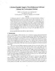
2.2 Boundary conditions The boundary C of the domain X is subdivided into nonoverlapping subsets Ce ; Cw and Cf , as shown in Figure 1, with boundary conditions:

a…v; u† ‡ …p; div u† ˆ 0

v ˆ ve vˆ0 pn
n ˆ 0

r
v‡

on Ce …entrance boundary† on Cw …non-slip boundary†

…2:9† …2:10† (2.11a)

on Cf …free surface boundary) pn
t ˆ 0

(2.11b)

…2:13†

The incompressibility condition (2.8), r
v ˆ 0, is enforced using the penalty method. This condition is reformulated as

p ˆ0 x

…2:14†

where x is a suf®ciently large penalty parameter. This is equivalent to introducing slight incompressibility. In order to formulate Equation (2.14) variationally, the space of pressure weighting functions Q is de®ned as follows:

Q ˆ fq : q 2 L2 …X†; q ˆ 0 on Cf g

Equations (2.11) are taken from the assumption of zero normal and shear stress, or zero stress vector, on the free Multiplying Equation (2.14) by an arbitrary q and intesurface boundary, and pn denotes the total stress vector on grating, Z Z a plane normal to the boundary. X

…r
v†q dX ‡

1 x

X

pq dX ˆ 0

…2:15†

or, in abstract form

b…div v; q† ‡ x1 …p; q† ˆ 0

Fig. 1. Illustration of the boundaries in the injection moulding ®lling process

…2:16†

Equations (2.13) and (2.16) represent the mixed variational problem. The system can be decoupled by substituting the pressure term in Equation (2.12) with Equation (2.14). This gives

Z

Z X

_ _ 2gc…v†
c…u† dX ‡

X

x…r
v†…r
u† dX ˆ 0 …2:17†

or, in abstract form,

a…v; u† ‡ x…div v; div u† ˆ 0 The variational problem is then formally posed as: Find v 2 U such that

a…v; u† ‡ x…div v; div u† ˆ 0

…2:18†

for all u 2 U where the space U is de®ned as before.

Owing to the incompressibility, or nearly incompressibility, condition present in the mixed formulation, mesh locking can occur. It is well known that only elements that satisfy the Babuska-Brezzi, or LBB, stability condition will not lock. Although the Q1 ÿ P0 element does not satisfy the LBB condition, optimal rate of convergence can still be proven under certain conditions which includes the elimination of the pressure degrees of freedom by way of the nearly incompressible approximation. In the solution of the equivalent formulation (2.18), four-noded quadrilateral elements are used with continuous bilinear velocity interpolation. The use of reduced (1-point) integration for the penalty term makes this scheme equivalent to the mixed formulation using the Q1 ÿ P0 element [Hughes (1987)].

This is, under certain conditions, equivalent to the mixed formulation. These restrictions are discussed in the 2.5 Finite Element formulation of the flow equation next section. In the Galerkin approximation, we de®ne the space Uh  U spanned by a ®nite dimensional basis Ni , i ˆ 1; 2; . . . ; n: 2.4 Both trial and weighting functions, vh and uh , belong to Proof of convergence this subspace. For convenience, the subscript h will be In the Galerkin approximation, the ®nite-dimensional h omitted, and all integrals henceforth are de®ned per elespace of velocity weighting functions U is de®ned such that Uh  U: Uh is spanned by the ®nite-dimensional basis ment and summed over all the elements of the discretised Niv ; i ˆ 1; 2; . . . ; n. Similarly, the subspace Qh of the space domain. The velocity vector is approximated by n X of pressure weighting functions Q can be de®ned, spanned p vˆ Ni vi ˆ Ne v by the ®nite-dimensional basis Nj ; j ˆ 1; 2; . . . ; m. iˆ1 Convergence of the approximate solutions vh 2 Uh and ph 2 Qh requires that where i is the node index, the Ni 's are the element interpolation functions, and vi is the nodal velocity vector. The 2 ÿ2gr …vh ÿ v† ‡ r…ph ÿ p† ˆ 0 …2:19† aim here is to express Equation (2.16) in ®nite element The weak variational form of the above equation can be form. To this end, the rate of deformation tensor is written written as in vector form as follows: Z 2 oNi 3 2 3 2 ov1 3 0   c_ 11 n ox1 ox1 2gr…vh ÿ v†
r…vh ÿ v† dX X v1 6 ov2 7 6 i 7 X ˆ Be v c_ ˆ 4 c_ 22 5 ˆ 4 @x 5ˆ 4 0 oN Z ox2 5 v 2 2 i ov1 ov2 oNi oNi i ˆ 1 _ c 12 …2:20† ÿ …ph ÿ p†r
…vh ÿ v† dX ˆ 0 @x2 ‡ ox1 ox2 ox1 X

after applying the relevant boundary conditions. Since p ˆ x…r
v† from the penalty function (2.14), Equation (2.20) can be rewritten as

Z

X

2gr…vh ÿ v†
r…vh ÿ v† dX Z 1 …ph ÿ p†…ph ÿ p† dX ˆ 0 ‡ Xx

r
v ˆ

n  ov1 ov2 X oNi ‡ ˆ ox1 ox2 ox1 iˆ1

oNi ox2



v1 v2



ˆ Ce v

Substituting the above two expressions into the variational ¯ow formulation (2.16) results in the following ®nite element formulation:

Z

or, in terms of the appropriate norms, as

2gkvh ÿ vk2H 1 ‡ x1 kph ÿ pk2H 0 ˆ 0

and the divergence of velocity, div v, is expanded as follows:

…2:21†

where H m is the space of functions which are square integrable up to their mth derivatives. From Equation (2.21), it is evident that, as x ! 1, vh ! v. Also, from Equation (2.19), as vh ! v, ph ! p. Thus, to ensure convergence, the bases N v and N p that span the function subspaces Uh  U and Qh  Q must be chosen such that the dimension of N p is less than that of N v . As an example, the Q1 ÿ P0 element conforms to this requirement. Continuous bilinear interpolation is used for the velocity ®eld and the pressure, or stress, ®eld is constant over the element.

X

BT DBe v dX ‡ x

Z X

CT Ce v dX ˆ 0

…2:22†

where D is the constitutive matrix.

3 Adaptive mesh refinement analysis 3.1 Convergence and mesh refinement In Section 2.4, the convergence of the ®nite element (approximate) solution vh to the exact solution v was considered. It was shown that, indeed, convergence can be

357

re®nement. It may be stated as follows: the residual calculated from the ®nite element solution converges to the exact residual of the continuous problem as the ®nite element mesh is re®ned. In problems which are in¯uenced by external body forces, the expression (3.6) still holds and the left hand side is an upper bound (as shall be shown later) for the residual. In the context of linear elasticity, only the ®rst 2 2 2gkvh ÿ vkH 1 ‡ x1 kph ÿ pkH 0 ! 0 as h ! 0 …3:1† bilinear form, referred to as the strain energy norm (or twice the strain energy norm), is present so that expression The expression (3.1) is, of course, equivalent to (3.6) can be stated as: the strain energy (norm) calculated 2gkvh ÿ vk2H 1 ‡ xkdiv vh ÿ div vk2H 0 ! 0 as h ! 0 from the ®nite element solution converges to the exact …3:2† strain energy (norm) of the continuous problem as the ®nite element mesh is re®ned. which can be written in inner product form as Although the overall re®nement of the ®nite element mesh (mesh enrichment) will result in a more accurate a…vh ÿ v; vh ÿ v† ‡ x…div vh ÿ div v; div vh ÿ div v† ! 0 solution, it will also lead to a larger stiffness matrix reas h ! 0 …3:3† sulting in longer computational times and greater storage demands. It is therefore computationally more practical to Consider the ®rst bilinear inner product of expression re®ne the mesh only in areas where the error is signi®cant (3.3) which can be expanded to give (selective mesh enrichment). a…vh ; vh † ÿ 2a…vh ; v† ‡ a…v; v† A more sophisticated re®nement strategy, in which the order of magnitude of the global stiffness matrix is apand noting that the error in the approximation is given by proximately maintained, is to adapt the mesh such that the e ˆ v ÿ vh , the above expression can be further developed error is equally distributed over all the elements. This to give involves re®ning the mesh in areas where the error is a…vh ; vh † ÿ 2a…vh ; vh ‡ e† ‡ a…v; v† greater than the average error and coarsening the mesh in areas where the error is smaller than the average error ˆ) a…vh ; vh † ÿ 2a…vh ; vh † ÿ 2a…vh ; e† ‡ a…v; v† (mesh adaptivity). This strategy will be illustrated in detail …3:4† in the implementation of the adaptive mesh re®nement ˆ) ÿa…vh ; vh † ÿ 2a…vh ; e† ‡ a…v; v† procedures to be developed later. Next, consider the second bilinear inner product of exAt this stage, it is important to note that, in the calcupression (3.3) which can be expanded to give lation of the error, the exact solution is required. This is x…div vh ; div vh † ÿ 2x…div vh ; div v† ‡ x…div v; div v† obviously not available. The most important aspect of an adaptive mesh re®nement procedure is therefore the estiand noting that the divergence of the error in the apmation of this error. proximation is given by div e ˆ div…v ÿ vh †, the above expression can be further developed to give ensured under particular choices of interpolation functions. However, no mention was made of the element size h which is central to the de®nition of convergence. While convergence is ensured, the exact solution is approached as the element size h is decreased. That is, vh ! v as h ! 0. Although this de®nition suf®ces, it is more appropriate, from Equation (2.21), to write

358

3.2 Error estimators for adaptive mesh refinement analysis

x…div vh ; div vh † ÿ 2x…div vh ; div vh ‡ div e† ‡ x…div v; div v† ˆ) x…div vh ; div vh † ÿ 2x…div vh ; div vh † ÿ 2x…div vh ; div e† ‡ x…div v; div v† ˆ) ÿx…div vh ; div vh † ÿ 2x…div vh ; div e† ‡ x…div v; div v†

3.2.1 The Babuska-Rheinboldt error estimator A framework for adaptive mesh re®nement analysis was ®rst developed by Babuska and Rheinboldt (1978) for …3:5† linear elastic analysis [see also Rannacher and Suttmeir Substituting the expressions (3.4) and (3.5) into the de®- (1997)] and the method was ®rst applied to non-Newnition for convergence (3.3) and using the orthogonality tonian Stokes ¯ow by Dannelongue and Tanguy (1990). condition between the error in the ®nite element approx- The detailed development and presentation of this method imation and the approximate solution (see Appendix A), is useful in the comparison of, and equivalence between, various methods. the result is Recall from Section 2.3 that the application of Green's theorem to the integral of the weighted Stokes formulation ÿa…vh ; vh † ‡ a…v; v† ÿ x…div vh ; div vh † resulted in ‡ x…div v; div v† ! 0 as h ! 0 Z Z or ÿ p : ru dX ‡ …n
p†
u dC ˆ 0 …3:7† a…vh ; vh † ‡ x…div vh ; div vh † ! a…v; v† ‡ x…div v; div v†

X

C

The boundary integral in Equation (3.7) is evaluated before the discretisation process. This effectively means that The above de®nition for convergence lays the foundation the value of this integral over the inter-element boundaries for the development of error estimates for adaptive mesh of the discrete domain is neglected.

as h ! 0

…3:6†

Owing to the C0 continuity of the velocity space, the total stress tensor p, which is a function of the velocity gradient, becomes discontinuous at the inter-element boundaries. The boundary integral therefore does not cancel out over the inter-element boundaries and its contribution to the error, as documented in literature, is far from negligible except for very ®ne meshes. For the Stokes problem, these extra boundary integrals, called inter-element jumps, is given by

bound for the inter-element jump Ji , where the starred values are computed in a neighbouring element. Error estimates based on the Babuska-Rheinboldt method such as that of Equation (3.11) are complex to evaluate because of the following reasons: ®rstly, they require the explicit determination of the inter-element traction jumps and, secondly, they involve integration along element interfaces.

X

3.2.2 The Zienkiewicz-Zhu error estimator Similar to the Babuska-Rheinboldt error estimator, the Zienkiewicz-Zhu error estimator is also based on the discontinuity of the stress at the inter-element boundaries due to the C0 continuity of the velocity space. However, this error estimator, although approximately equivalent [(Zienkiewicz and Zhu (1987)] to that of Babuska-Rheinboldt, is computationally much simpler to evaluate. The method was ®rst developed for the linear elasticity problem by Zienkiewicz and Zhu (1987). It has subsequently been applied to many different types of both linear and non-linear problems, including that of non-linear forming processes [Onate and Bugeda (1993)]. The aim here is to develop an expression for the elemental error estimate keki for the non-Newtonian Stokes problem using the method of Zienkiewicz and Zhu. The energy dissipation norm is de®ned in the context of the Stokes problem as  Z 1=2 1 kvk ˆ p : c_ dX …3:12† 2 X

Ji ˆ

i

XZ

Ii

i

ˆ



XZ

Ii

i

…n
p†
u dI  n
…pd ‡ s†
u dI

…3:8†

where Ii refers to the boundary of element i. Equation (3.8) can be expanded as follows:

X

Ji ˆ

i

ˆ ˆ

XZ



i

Ii

i

Ii

i

Ii

XZ XZ

…pn ‡ sn †
u dI  n
…pn ‡ sn †u
n ‡ t
…pn ‡ sn †u
t dI  …p ‡ snn †u
n ‡ …snt †u
t dI

…3:9†

In any adaptive process, the re®nement of the mesh should be driven by the local (elemental) value of the error norm, as discussed in the previous section. Since the value of the exact norm is not available, estimates of the error norm can be derived a posteriori from the solution. The proper norm in which to express the error for the Stokes problem is the H 1 semi-norm for velocity and the L2 …H 0 † norm for pressure since these are the spaces in which the velocity and pressure ®elds were sought (see Section 2.3). Furthermore, it is a natural choice to base the error estimate on the residual since this takes into account the inter-element jumps and is also an upper bound for the global error when the elements satisfy the Babuska-Brezzi compatibility condition. But since the residual is de®ned in the dual space, its norm (see Equation 2.20) is cumbersome to evaluate. A more practical error estimate leads to the following upper bound for the global error:

" kek ˆ

X i

#1=2 kek2i

…3:10†

where the elemental contribution for an element of mesh size h is given by

(

2 kek2i ˆ C h2 gr2 v ÿ rp ‡

X

hj…p ‡ snn † ÿ …p ‡ snn † j

kvk ˆ

 Z 1=2 Z 1 1 s : c_ dX ‡ pd : c_ dX 2 X 2 X

and noting that s is given by the constitutive equation (2.3) _ as ÿ2gc,

 Z 1=2 Z 1 1 kvk ˆ ÿ2gc_
c_ dX ‡ pr
v dX 2 X 2 X

where the tensor c_ has been written in equivalent vector form. Substituting for p from Equation (2.13),

kvk ˆ

 Z 1=2 Z 1 1 ÿ2gc_
c_ dX ÿ x …r
v†…r
v† dX 2 X 2 X …3:13†

The absolute value of the integral is implied and its sign will therefore be ignored. Equation (3.13) can be written in abstract form as

)  2

where c_ the rate of deformation tensor and p is the total stress tensor de®ned previously as pd ‡ s where s is the deviatoric stress tensor. Substituting for p, Equation (3.12) becomes

…3:11†

Ii

The ®rst term, the elemental residual, is an upper bound for the elemental error. The second term is an upper

kvk2 ˆ 12a…v; v† ‡ 12x…div v; div v†

…3:14†

In the ®nite element approximation, c_ ˆ Be v and r
ˆ Ce v where the tilda …e† refers to a nodal vector and the matrices B and C are given in Section 2.5. The elemental energy norm therefore becomes

359

 Z 1=2 Z 1 1 T T T T e e kvki ˆ v dX ‡ x v dX v B 2gBe v C Ce 2 Xi 2 Xi …3:15† Using the above equation, the error energy norm can be constructed as follows:

kv ÿ vh ki ˆ 360

1 2

Z

Xi

vÿe vh †T BT 2gB…e …e vÿe vh † dX

1 ‡ x 2

!1=2

Z Xi

…e vÿe vh †T CT C…e vÿe vh † dX

or, in terms of the error, as

 Z 1=2 Z 1 1 T T T T e e keki ˆ B 2gBee dX ‡ x C Cee dX 2 Xi 2 Xi …3:16† Note that the (pointwise) error e in the above equation refers to the error in the velocity. Since the exact solution of the velocity ®eld is not known, this form of the elemental error norm is not useful. It will be more useful if the error in the stress ®eld is introduced. Although the exact stress ®eld is also not known, the aim is to smooth the globally discontinuous approximate stress ®eld, ph , to obtain a better approximation of the stress ®eld. Equation (3.16) can therefore be rewritten as Z 1 keki ˆ …2gBee†T …2g†ÿ1 …2gBee† dX 2 Xi !1=2 Z 1 T ÿ1 …xCee† …x† …xCee† dX ‡ 2 Xi

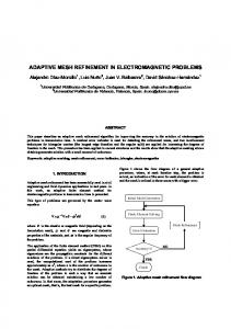
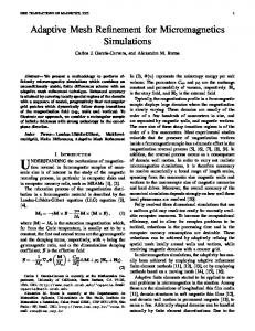
Figure 2, it is intuitive that s is a better approximation than sh , so that s  s. The smoothed approximate stress ®eld, s , is interpolated in the same way as vh (globally continuous), that is

s ˆ Nes

…3:18†

where N is the matrix of interpolation functions used in the ®nite element solution of the Stokes problem. For the two-dimensional problem, there are three independent stress components and, for the four-noded quadrilateral element, es can be represented as a nodal vector with 12 elements. In this case, N becomes a 3  12 matrix. The nodal vector es can be found by realising that the integral of the error must vanish, that is

Z

X

…s ÿ sh † dX ˆ 0

…3:19†

Substituting the discrete forms of the stress tensor gives

Z

X

…Nes ÿ …ÿ2g†Be vh † dX ˆ 0

Multiplying by NT and rearranging gives the desired explicit formula for es :

es ˆ ÿAÿ1

Z

X

ÿ T
N 2gB dXe vh

…3:20†

where

Z

Aˆ

X

NT N dX

…3:21†

To summarise, the global nodal vector es can be determined using Equation (3.20) and substituted into Equation (3.17) to determine the elemental error estimate.  Z 1=2 As in the case of the Babuska-Rheinboldt error esti1 eTs …2g†ÿ1es ‡ eTp …x†ÿ1ep d X ˆ …3:17† mators, the Zienkiewicz-Zhu error estimator also requires 2 Xi the posteriori calculation of the nodal stresses. Although the integration of the inter-element stress jumps along the  where the nodal error vectors es ˆ es ÿ esh and ep ˆ inter-element faces is not explicitly performed, the evalue ph . The aim now is to compute the nodal vectors es ation of the smoothed nodal stress vector, es , using p ÿ e and e p . This procedure will be illustrated for es only, and Equation (3.19) is an equivalent procedure. In fact, the the same procedure can be followed to determine e p . From equivalence of the two error estimators is proven by Zienkiewicz and Zhu (1987). What is evident, though, is that the Zienkiewicz-Zhu error estimator is much easier to evaluate within existing ®nite element code because it makes use of ``standard'' matrix forms and numerical procedures.

3.2.3 A new error estimator based on Strain Energy Equalisation For the discrete problem, the energy norm of the exact solution can be written in terms of the pointwise de®nition of the error, e ˆ v ÿ vh , as a…v; v† ‡ x div…v; div v† ˆ a…e ‡ vh ; e ‡ vh † ‡ x…div…e ‡ vh †; div…e ‡ vh ††

…3:22†

Using the bilinearity of the inner products, the above

Fig. 2. Illustration of the error for C0 continuous (bi)linear interpolation functions, adapted from Zienkiewicz and Zhu (1987) equation can be expanded to give

a…v; v† ‡ x div…v; div v† ˆ a…e; e† ‡ 2a…e; vh † ‡ a…vh ; vh † ‡ x…div e; div e† ‡ 2x…div e; div vh † ‡ x…div vh ; div vh † and, using the orthogonality condition developed in Appendix A, this simpli®es to

a…v; v† ‡ x…div v; div v† ˆ a…e; e† ‡ x…div e; div e† ‡ a…vh ; vh † ‡ x…div vh ; div vh †

Using the bilinearity of the inner product, this can be expanded to give

 kek  cha a…vh ; vh † ‡ 2a…vh ; e† ‡ a…e; e† ‡ x…div vh ; div vh † ‡ 2x…div vh ; div e† 1=2 ‡ x…div e; div e†

and using the orthogonality condition developed in Appendix A, the above reduces to

…3:23†

Equation (3.23) is analogous to the de®nition of convergence developed earlier, given by expression (3.6). The only difference here is that the error is explicitly introduced. Rearranging Equation (3.23) slightly as follows:

 kek  cha a…vh ; vh † ‡ a…e; e† ‡ x…div vh ; div vh † 1=2 ‡ x…div e; div e† or,

 1=2 kek  cha kvh k2 ‡ kek2

…3:26† a…e; e† ‡ x…div e; div e† ˆ a…v; v† ‡ x …div v; div v† Finally, writing the inequality (3.26) as ÿ a…vh ; vh † ‡ x…div vh ; div vh † kek  cha …3:27† It is clear that the error in the energy is equal to the energy  2 2 1=2 kvh k ‡ kek of the error. Furthermore, since the inner products, or norms, are all positive de®nite, the property: it is clear that the relative (square of the) error norm is bounded. This also means that the error norm is related to a…vh ; vh † ‡ x…div vh ; div vh †  a…v; v† ‡ x …div v; div v† the energy norm of the approximate solution, resulting in …3:24† an elemental error estimate of the form: can be deduced. This states that the energy norm of the s 2 approximate solution is bounded above by that of the …chai † …3:28† exact solution. In other words, the approximation method kek  2 kv h ki a 1ÿ…chi † over-estimates the ``stiffness'' of the system. The understanding of this is important for the forthcoming discussion. That is, the energy norm of the approximate solution In terms of adaptive mesh re®nement, this effectively always approaches the energy norm of the exact solution implies the equalisation of the energy norm of the apfrom below, with a certain rate of convergence as the mesh proximate solution. This is intuitive in a sense that larger absolute errors are normally expected in regions where the size is re®ned. Instead of Equation (3.24), the following inequality can solution gradients are larger. be written: 3.3 a…e; e† ‡ x…div e; div e†  a…v; v† ‡ x…div v; div v† A general adaptive mesh refinement strategy or, in terms of the norms, and introducing discretisation As was mentioned earlier, adaptive mesh re®nement involves the equalisation or equilibration of the elemental parameters, error norm. The aim of this section is therefore to develop a kek  ch kvk …3:25† a general mesh re®nement strategy which will achieve this where c is a constant independent of v and h, and a de- equalisation. Furthermore, a general strategy will be depends on the degree of highest complete polynomial of the veloped which can be employed with any of the error estimators developed previously. element interpolation functions and the order of the Similar to Equation (3.25), the fundamental error estihighest derivatives appearing in the bilinear term of the mate for elliptic boundary value problems is stated as weak variational form (or the energy expression). The exponent a can be found from …k ‡ 1 ÿ m† where k is the follows: degree of completeness of the interpolation functions and kek  chk‡1ÿm kvk …3:29† m is the order of the weak variational form. The above inequality is also known as the fundamental error estimate where c is a constant independent of v and h, k is the degree of polynomial completeness of the element interfor elliptic boundary value problems [Hughes (1987), polation functions, and m is the order of the highest deBathe (1996)]. rivatives appearing in the bilinear term of the weak The inequality (3.25) can be written as variational form (or the energy expression). For the Stokes a kek  ch kvh ‡ ek problem using the standard 4-noded bilinear conforming element, m ˆ 1 and k ˆ 1, such that and writing the norm in the inner product form gives  kek  chkvk …3:30† kek  cha a…vh ‡ e; vh ‡ e† 1=2 It is clear that, from Equation (3.30), the convergence of ‡ x…div…vh ‡ e†; div…vh ‡ e†† the error is of the order O…h†. Equation (3.30) is more

361

useful if we introduce the maximum permissible relative error e such that

eˆ

kv ÿ vh k kvk

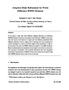
The value of e is chosen according to the desired accuracy. The smaller the value of e, the ®ner the mesh and, consequently, the more accurate the solution. Equation (3.30) Fig. 3. Con®guration of the model problem can therefore be written as 362

kek ˆ ekvk Substituting for v in terms of its approximation and corresponding error,

kek ˆ ekvh ‡ ek Writing the right hand side norm in the inner product form, expanding this bilinear form, and using the orthogonality condition developed in Appendix A, the above can be written as

 1=2 kek ˆ e kvh k2 ‡ kek2

…3:31†

Now, given that K is the number of elements in the mesh, the maximum permissible error per element becomes

" #1=2 kvh k2 ‡ kek2 kekp ˆ e K

…3:32†

As the elemental error keki is computed for each element (as illustrated for the various methods in the previous section), it can be readily checked where re®nement is necessary by comparing this elemental error to the permissible error kekp . If hi is the current element size for element i, and knowing that the convergence of the ®nite element solution to the exact solution (and hence the convergence of the error to zero) is of the order ha , then the predicted element size, h, can be found using the following:

 a hi keki ˆ h kekp

…3:33†

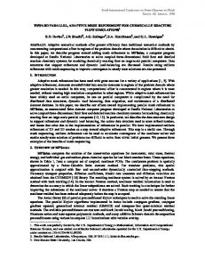
Model given by Equation (2.7) with the following material constants: power law index n ˆ 0:2799, transition stress s ˆ 1:484  104 , B ˆ 5  108 , temperature constant Tb ˆ 1:352  104 , and b ˆ 3:5  10ÿ8 , all in SI units. Using a mesh density of 2 mm, the ®lling process was simulated until the cavity was 14.20% full. The ¯ow domain at this stage is illustrated in Figure 4. The mesh was then adapted, with zero reduction in the global error, using both the Zienkiewicz-Zhu (Z-Z) error estimator and the Strain Energy Equalisation (SEE) error estimator. An upper limit of 3 mm and a lower limit of 1 mm is placed on the mesh density. This is to avoid the occurrence of highly distorted elements. The results, after the ®rst adaptive iteration, are shown in Figure 5. Table 1 compares the performance of the two methods. The energy norm is used as a performance indicator. The higher the energy norm, the more accurate the solution since the energy norm is bounded above by that of the exact solution. It is clear that the methods compare very well. In fact, the new SEE error estimator performs slightly better with a higher energy norm and fewer elements. A second adaptive analysis was performed on the original mesh, this time with a 25% reduction in the global error. The results, after 1 adaptive iteration, is shown in Figure 6. Table 1 shows no signi®cant improvement in the results because of the upper and lower limits set on the mesh density. The methods again compare very favourably. The new method again results in fewer elements.

4.2

The elemental error may be greater than or less than the Non-Newtonian flow into a mould cavity permissible error, indicating whether the new mesh should In the example problem, polymer melt at a temperature of 200 C and with the same viscosity characterisation as that be re®ned or coarsened. That is:  in the previous example, is injected into the mould cavity > 1; h refined shown in Figure 7. A ®lling time of 1 second is speci®ed. keki =kekp ˆ

< 1;

h coarsened

The mesh re®nement procedure can now be effected using Equations (3.32) and (3.33), together with the speci®c elemental error estimate employed, either Equation (3.11), (3.17) or (3.28).

4 Numerical results 4.1 Comparison between the Z-Z and SEE error estimators The ¯ow of polystyrene PS DOW Styron 685 through a thin cavity, shown in Figure 3, was simulated. The material Fig. 4. Flow domain at 14.2% ®lled. Unadapted mesh with mesh density of 2 mm non-linearity was modelled using the Cross-Exponential

Fig. 5a, b. The adapted domain with zero global error reduction Fig. 6a, b. The adapted domain with 25% global error reduction using a the Zienkiewicz-Zhu error estimator and b the Strain using a the Zienkiewicz-Zhu error estimator and b the Strain Energy Equalisation error estimator Energy Equalisation error estimator

In injection moulding practice, appropriate ram speed pro®les are speci®ed to ``balance'' the ¯ow and prevent adverse effects at sudden expansions and contractions. For the example problem, the ram speed pro®le shown in Figure 8 is used. A slower ram speed during the ®rst quarter of the cycle allows the polymer melt to emerge from the gate with a lower melt front velocity. When the melt front area has reached a big enough value, the ram speed is increased. The given ram speed pro®le can be used to determine the injection rates. The horizontal axis can be interpreted as the ®lled volume and the vertical axis as the injection Fig. 7. Geometry for the mould ®lling simulation example with rate. The maximum injection rate IRmax can then simply be initialised melt front. Dimensions (in mm): gate ± 10  2  2:00 runner ± 10  28  2:00 found as follows:

25% of cavity volume 75% of cavity volume ‡ 0:5…IRmax † …IRmax † ˆ fill time

domain at various stages in the ®lling process. A maximum of 817 nodes and 731 elements is generated when the cavity is completely ®lled.

Since the cavity volume is 5600 mm3 and the ®ll-time is 1 second, the maximum injection rate IRmax ˆ 7000 mm3 =s. This translates to inlet velocities of 175 mm/s for the ®rst quarter of the ®lling cycle and 350 mm/s for the rest of the ®lling cycle. The melt front is initialised immediately before the gate, as shown in Figure 7. This occurs at 10.0% of the total ®lling process. A time step of 0.005 seconds is used to explicitly advance the melt front. At each time step, the domain is remeshed, and the velocity ®eld is solved using the non-linear ¯ow formulation. On the average, the solution converges to within 1 percent after four NewtonRaphson iterations. The simulation is carried out for two cases: (a) without adaptive mesh re®nement and (b) with adaptive mesh re®nement. The results are discussed below.

(b) Simulation with adaptive mesh re®nement In the second case, adaptive mesh re®nement analysis is used to optimise the mesh. The error estimate (3.28) based on the equalisation of the strain energy is used in conjunction with the re®nement strategy outlined in Section 3.3. In the calculation of the elemental error estimates according to Equation (3.28), the value of h is chosen as the mesh size of the initialised mesh, that is, h ˆ 2 mm. The value of the constant c is chosen such that the elemental error norm keki is a reasonable fraction of the elemental strain energy norm kvki . In this case, c ˆ 0:1 is used, and since a ˆ 1, cha ˆ 0:2. Equation (3.28) which describes the error estimate and Equation (3.32) which de®nes the maximum permissible error per element, are derived from the same source. It is therefore clear that the value of the (a) Simulation with uniform mesh density re®nement parameter e is the same as that for cha . If a In the ®rst case, a uniform mesh density of 2 mm is used reduction in the error is sought, then e can be multiplied throughout the domain. Figure 9(a)±(f) shows the meshed by a factor less than 1 according to the desired accuracy. In Table 1. Comparative data for the adaptive mesh re®nement analysis using the two different error estimators

number of elements % permissible error e energy norm kvh kX

original

Z-Z

SEE

Z-Z (0.75e†

SEE (0.75e†

72 24.16 2161.83

83 21.61 2507.07

78 21.61 2564.74

104 22.97 2552.16

93 22.97 2529.46

363

364

It is evident from Figure 10 that, in the case of the adapted mesh, the element sizes are smaller in areas of high shear rate, such as near the corners and at the entrance to the mould. The free surfaces generated compare very well with that of the uniform mesh. This is con®rmed by the free surface plots shown in Figure 11. A quantitative comparison is given by the data in Table 2. As mentioned previously, the strain energy of the approximate solution is an indicator of the accuracy of the solution. Since the mesh was adapted with zero error reduction, the values of strain energy for Fig. 8. The ram speed pro®le for the mould ®lling simulation the uniform and adapted meshes are therefore almost the same. A 3±4% variation in strain energy is common at this case, an optimisation of the mesh density distribution different time steps, and is a consequence of numerical approximation. is sought, with no reduction in the error. The aim is to The advantage of adaptive mesh re®nement lies in the investigate the effect of the adaptive analysis on the number of elements, and, hence, the computational time. reduction of the number of nodes. Since the computaThe lower and upper limits of the mesh density is set to tional effort is a function of the square of the number of nodes, the 33% reduction in the number of nodes for the 1.5 mm and 3 mm respectively, to prevent undesirable same solution accuracy is a clear indication of the addistortion of elements. The results are shown in Figure vantage of the adaptive mesh re®nement. 10(a)±(f) at comparable stages to that of the previous simulation.

Fig. 9a±f. Various stages in the mould ®lling process for the example problem of Figure 7 with uniform mesh density at a u ÿ t ˆ 0:20, b t ˆ 0:35, c t ˆ 0:50, (d) t ˆ 0:65. e t ˆ 0:80, f t ˆ 0:95

365

Fig. 10a±f. Various stages in the mould ®lling process for the example problem of Figure 7 with adaptive mesh re®nement at a t ˆ 0:20, b t ˆ 0:35, c t ˆ 0:50, d t ˆ 0:65, e t ˆ 0:80, f t ˆ 095

5 Conclusions In the Galerkin ®nite element method, the error estimators developed by Babuska and Rheinboldt and Zienkiewicz and Zhu are expressed in terms of the inter-element discontinuity of the solution gradient (for C0 continuity of the solution ®eld). This requires the a posteriori calculation of the solution gradient. In the present method, the error

estimator is developed in terms of the approximation solution ®eld (or its appropriate norm). This is simply achieved by using the boundedness and orthogonality conditions applicable to the Galerkin ®nite element method. The error is therefore estimated in the solution space, obviating the need for the a posteriori calculation of the solution gradient. In essence, the new error estimator implies that the error in the solution is proportional to the energy norm of the approximate solution. In terms of the discrete problem, this means that elements with higher energy norms will produce higher errors. As the element size is reduced, its energy norm is likewise reduced, leading to a reduced Table 2. Comparison data for the two simulations of the example problem at t ˆ 0:95

Fig. 11. Comparison of the free surfaces produced by the two simulations of the example problem

Uniform mesh Adapted mesh

Number of nodes

Number of elements

Strain energy (kJ/s)

788 531

706 456

10.446 10.043

366

error. This is obvious in terms of the convergence requirement for ®nite element solutions. In terms of optimising the mesh density, the new error estimator implies the equal distribution of the energy norm of the approximate solution. That is, element sizes are adjusted so that the individual elements produce equivalent norms. The accuracy of the new error estimator, based on the elemental equalisation of strain energy, has been shown to perform favourably when compared to Zienkiewicz-Zhu error estimator. The new error estimator, besides requiring less a posteriori computational effort, also produces fewer elements. The new error estimator has been applied to the injection mould ®lling process, modelled by the incompressible Stokes ¯ow formulation, resulting in a signi®cant reduction in element numbers.

than in Uh ). Indeed, any solution v to Equation (A.3) is also a solution of Equations (A.1) and (A.2). Subtracting Equation (A.2) from Equation (A.3) gives

a…v;uh † ÿ a…vh ; uh † ‡ x…div v; div uh † ÿ x…div vh ; div uh † ˆ 0

(A.3)

and, using the bilinearity of the above inner products,

a…v ÿ vh ; uh † ‡ x…div v ÿ div vh ; div uh † ˆ 0 ) a…v ÿ vh ; uh † ‡ x…div …v ÿ vh †; div uh † ˆ 0 ) a…e; uh † ‡ x…div e; div uh † ˆ 0 This means that the error and its divergence in the approximation of the velocity are orthogonal to the subspace Uh and its divergence, respectively. Since, in the Galerkin approximation method, the trial functions vh also belong to Uh , it is therefore evident that the error and its divergence are also orthogonal to the solution and its divergence, respectively. That is:

Appendix An orthogonality condition for the Galerkin a…e; vh † ‡ x…div e; div vh † ˆ 0 (A.4) approximation method Consider the weak formulation of the Stokes ¯ow problem (Equation 2.16): References Find v 2 U such that Babuska I, Rheinboldt WC (1978) Error estimates for adaptive a…v; u† ‡ x…div v; div u† ˆ 0

(A.1)

for all u 2 U where the space U is de®ned as follows:

 U ˆ u ˆ …u1 ; u2 † : u1 ; u2 2 H1 …X†; u ˆ 0 on Ce [ Cw The approximate ®nite element problem can be stated analogously as: Find vh 2 Uh such that

a…vh ; uh † ‡ x…div vh ; div uh † ˆ 0 h

(A.2) h

for all uh 2 U where the space U  U. Since Uh  U, Equation (A.1) can be written as

a…v; uh † ‡ x…div v; div uh † ˆ 0

(A.3)

That is, the weighting functions now lie in the ®nitedimensional subspace Uh while the trial solution space is still U (the exact solution v is most probably in U rather

®nite element computations, SIAM J. Num. Analysis, 15:4 Bathe K-J (1996) Finite Element Procedures, Prentice-Hall, New Jersey Brink U, Stein E (1997) ``On some mixed ®nite element methods for incompressible and nearly incompressible ®nite elasticity'' Computat. Mech. 19:105±119 Dannelongue HH, Tanguy PA (1990) An adaptive remeshing technique for non-Newtonian ¯uid ¯ow, Int. J. Num. Meth. Eng. 30:1555±1567 Hughes TJR (1987) The Finite Element Method, Prentice-Hall Onate E, Bugeda G (1993) A study of mesh optimality criteria in adaptive ®nite element analysis. Eng. Comput. 10:307±321 Rannachar R, Suttmeir F-T (1997) ``A Feed-back approach to error control in ®nite element methods: application to linear elasticity'' Computat. Mech. 19:434±446 Zienkiewicz OC, Zhu JZ (1987) A Simple Error Estimator and Adaptive Procedure for practical Engineering Analysis, Int. J. Num. Meth. Eng. 24:337±357