An Experimental Investigation of Model-Based Parameter Optimisation

An Experimental Investigation of Model-Based Parameter Optimisation: SPO and Beyond Frank Hutter

Holger H. Hoos

Kevin Leyton-Brown

Kevin P. Murphy

Department of Computer Science, University of British Columbia 201-2366 Main Mall, Vancouver BC, V6T 1Z4, Canada

{hutter, hoos, kevinlb, murphyk}@cs.ubc.ca Categories and Subject Descriptors I.2.8 [Artificial Intelligence]: Problem Solving, Control Methods, and Search—Heuristic methods; G.3 [Probability and Statistics]: Experimental design; G.1.6 [Numerical Analysis]: Optimization—Global optimization

General Terms Algorithms, Design, Experimentation, Performance

Keywords Parameter Tuning, Noisy Optimization, Sequential Experimental Design, Gaussian Processes, Active Learning

ABSTRACT This work experimentally investigates model-based approaches for optimising the performance of parameterised randomised algorithms. We restrict our attention to procedures based on Gaussian process models, the most widely-studied family of models for this problem. We evaluated two approaches from the literature, and found that sequential parameter optimisation (SPO) [4] offered the most robust performance. We then investigated key design decisions within the SPO paradigm, characterising the performance consequences of each. Based on these findings, we propose a new version of SPO, dubbed SPO+ , which extends SPO with a novel intensification procedure and log-transformed response values. Finally, in a domain for which performance results for other (model-free) parameter optimisation approaches are available, we demonstrate that SPO+ achieves state-of-the-art performance.

1.

INTRODUCTION

Many high-performance algorithms—and in particular, many heuristic solvers for computationally challenging problems—expose a set of parameters that allow end users to adapt the algorithm to a specific target application. Optimising parameter settings is thus an important task in the context of developing, evaluating and applying such algorithms. Recently, a substantial amount of research has aimed at defining effective, automated procedures for parameter optimisation (also called algorithm configuration or parameter Permission to make digital or hard copies of all or part of this work for personal or classroom use is granted without fee provided that copies are not made or distributed for profit or commercial advantage and that copies bear this notice and the full citation on the first page. To copy otherwise, to republish, to post on servers or to redistribute to lists, requires prior specific permission and/or a fee. GECCO’09, July 8–12, 2009, Montréal Québec, Canada. Copyright 2009 ACM 978-1-60558-325-9/09/07 ...$5.00.

tuning). More formally, given a parameterised target algorithm A, a set (or distribution) of problem instances I and a performance metric c, the goal is to find parameter settings of A that optimise c on I. The performance metric c is often based on the runtime required to solve a problem instance or, in the case of optimisation problems, on the solution quality achieved within a given time budget. Several variations of this problem have been investigated in the literature. First, these formulations vary in the number and type of target algorithm parameters allowed. Much existing work deals with relatively small numbers of numerical (often continuous) parameters (see, e.g., [11, 2, 1]); some relatively recent approaches permit both larger numbers of parameters and categorical domains (see, e.g., [17, 9, 16]). Second, approaches differ in whether or not explicit models (so-called response surfaces) are used to describe the dependence of target algorithm performance on parameter settings. There has been a substantial amount of work on both model-free and model-based approaches. Some notable model-free approaches include F-Race by Birattari et al. [9, 3], the C ALIBRA procedure by Adenso-Diaz & Laguna [1], and ParamILS by Hutter et al. [17]. State-of-the-art model-based approaches use Gaussian stochastic processes (also known as ‘kriging models’) to fit a response surface model. These models minimise the mean squared error between predicted and actual responses, using a non-parametric function to represent the mean. Combining such a predictive model with sequential decisions about the most promising next design point (based on a so-called expected improvement criterion) gives rise to a popular and widely studied approach in the statistics literature, which is known under the acronym DACE (Design and Analysis of Computer Experiments [21]). An influential contribution in this field was the Efficient Global Optimisation (EGO) procedure by Jones et al. [19], which addressed the optimisation of deterministic black-box functions. Two independent lines of work extended EGO to noisy functions: the sequential kriging optimisation (SKO) algorithm by Huang et al. [15], and the sequential parameter optimisation (SPO) procedure by Bartz-Beielstein [5, 4]. In our study of model-based optimisation of randomised target algorithms, we maintain this focus on Gaussian process (GP) models. We also limit ourselves to the simple case of only one problem instance (which may be chosen as representative of a set or distribution of similar instances). We make this restriction because, while still retaining significant practical relevance and focusing on core conceptual issues, it allows us to avoid the problem of performance variation across a set or distribution of problem instances. (The management of such variation is an interesting and important topic of study; indeed, we have already begun to investigate it in our ongoing work. We note that this problem can be addressed by the algorithm of Williams et al. [25], though only in the case of deterministic target algorithms.)

We thoroughly investigate the two fundamental components of any model-based optimisation approach in this setting: the choices taken in building the predictive model, and the sequential procedure that uses this model to find performance-optimising parameter settings of the target algorithm. First, in Section 2, we describe our experimental setup, with a special focus on the two target algorithms we consider, CMA-ES [14, 13] and SAPS [18]. In Section 3, we compare the two model-based optimisation procedures SKO and SPO. Overall, we found that SPO produced more robust results than SKO in terms of the final target algorithm performance achieved. Consequently, we focused the remainder of our study on the mechanisms that underly SPO. In Section 4, we investigate the effectiveness of various methods for determining the set of parameter settings used for building the initial parameter response model. Here we found that using more complex initial designs did not consistently lead to improvements over more naïve methods. More importantly, we also found that parameter response models built from log-transformed performance measurements tended to be substantially more accurate than those built from raw data (as used by SPO [4]). In Section 5, we turn to the sequential experimental design procedure. We introduce a simple variation in SPO’s intensification mechanism which led to significant and substantial performance improvements. Next, we consider two previous expected improvement criteria for selecting the next parameter setting to evaluate, and derive a new expected improvement criterion specifically for optimisation based on predictive models trained on logarithmic data. This theoretical improvement, however, did not lead to consistent improvements in algorithm performance. Finally, we demonstrate that our novel variant of SPO, which we dub SPO+ , achieved an improvement over the best previously-known results on the SAPS parameter optimisation benchmark.

2.

TARGET ALGORITHMS AND EXPERIMENTAL SETUP

The target algorithms we used in our study of model-based parameter optimisation procedures are CMA-ES and SAPS. CMA-ES is a prominent gradient-free global optimisation algorithm for continuous functions [14, 13] which is based on an evolutionary strategy that uses a covariance matrix adaptation scheme. We used the Matlab implementation CMA-ES 2.54,1 which is integrated into the SPO toolbox version 0.4 and was used as an example application for parameter optimisation in the SPO manual [6]. CMA-ES has two obvious parameters: the number of parents, N , and a factor ν ≥ 1 relating the number of parents to the population size. (The population size is defined as bN × ν + 0.5c.) Furthermore, Bartz-Beielstein et al. [6] modified CMA-ES’s interface to expose two additional parameters: the “learning rate for the cumulation for the step size control”, cσ or cs, and the damping parameter, dσ or damps (for details, see [12]). We used exactly the same region of interest (see Table 1) considered in Bartz-Beielstein et al.’s SPO example based on CMA-ES [6]. For each run of CMA-ES, we allowed a limited number of function evaluations and used the resulting solution quality (i.e., the minimal function value found) as the response variable to be optimised. We considered four canonical 10-dimensional test functions with a global minimum function value of zero that have previously been used for the evaluation of CMA-ES: the Sphere function (used in the SPO example mentioned above) and the Ackley, Griewank, and Rastrigin functions (as used by Hansen & Kern [13]). For the 1 The newest CMA-ES version, 3.0, differs mostly in the interface and in supporting “separable” CMA (see the change log at http://www.lri.fr/~hansen/cmaes_inmatlab.html).

Target algorithm Parameter Domain N [1, 50] CMA-ES ν [2, 10] cs (0, 1] damps [0.25, 0.99] α (1, 1.4] SAPS ρ [0, 1] Psmooth [0, 0.2] wp [0, 0.06]

Type integer continuous continuous continuous continuous continuous continuous continuous

Table 1: Target algorithms, parameters, and the regions of interest (parameter domains) considered. first three functions, we optimised mean solution quality reached by CMA-ES within 1 000 function evaluations, while for the more challenging Rastrigin function we set a limit of 10 000 function evaluations. The second target algorithm we considered was SAPS [18], a high-performance dynamic local search algorithm for the propositional satisfiability problem. We used the standard UBCSAT implementation [24] of SAPS and defined the region of interest (see Table 1) closely following Hutter et al.’s earlier parameter optimisation study using SAPS [17], with the difference that we did not discretise parameter values. (Hutter et al. did so because the parameter optimisation procedure used by them required it.) For SAPS, our goal was to minimise the median run-time (measured in local search steps) for solving the “quasigroups with holes” (QWH) SAT instance used in [17]. This instance belongs to a family of distributions that has received considerable interest in the SAT community. We chose this particular instance to facilitate direct comparison of the performance achieved by the parameter optimisation procedures considered here and in [17]; of course, we cannot draw general conclusions about optimising SAPS from studying a single instance. To evaluate the quality Q(θ) of a proposed parameter setting θ in an offline evaluation stage of the algorithm, we always performed additional test runs of the target algorithm with setting θ. In particular, for the CMA-ES test cases, we computed Q(θ) as the mean solution quality achieved by CMA-ES using θ across 100 test runs. For the higher-variance SAPS domain, we computed Q(θ) as the median runtime achieved by SAPS with setting θ across 1 000 test runs. We measure the performance pk of a parameter optimisation run after k runs of the target algorithm as the performance Q(θ) of the parameter setting θ the method would output if terminated at that point. The final performance of a parameter optimisation run is the performance at the end of the run. In order to measure the performance of a parameter optimisation method, we performed 25 runs of the method with different random seeds, and report mean and standard deviation of the final performance across these 25 repetitions. We also performed paired signed rank tests for differences in final performance (we chose a paired test because, using identical random seeds, the ith repetition of every parameter optimisation method used the same initial design and response values). For the experiments in Section 5.3 this pairing did not apply, so there we used the (unpaired) Mann-Whitney U test.

3.

SEQUENTIAL MODEL-BASED OPTIMISATION METHODS: SKO VS SPO

As discussed in the introduction, the two most influential existing methods for model-based optimisation of noisy functions (such as the performance of a randomised algorithm) are the SKO algorithm of Huang et al. [15] and the SPO framework of BartzBeielstein et al. [5, 4]. We unify both through the general framework presented as Algorithm 1. Both methods first generate an initial Latin hypercube design (LHD) and evaluate the respective

SKO SPO 0.3 SPO 0.4

−5

k

10

performance p

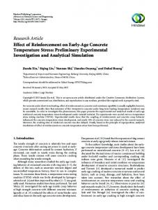
parameterisations of the target algorithm. (For a D-dimensional parameter optimisation task, SKO performs an additional run for the D parameter settings with the lowest response in this LHD; in SPO’s initial design, r repeats are performed for each point, where r is a parameter we fixed to its default value of 2 in this study.) Both methods then iterate through the following steps: fit a Gaussian process model M to predict the response for all parameter settings; select an incumbent parameter setting (to be returned upon termination); based on the predictive model M and an expected improvement criterion, select one or more new parameter settings and evaluate them. The two methods differ in their implementation of these steps. Before fitting its Gaussian process model, SPO computes empirical estimates of the user-defined performance metric (e.g., mean solution quality) at each previously-observed parameter setting; it then fits a noise-free Gaussian process model to this data. Since this model is noise-free, it perfectly predicts on its training data and the incumbent selected in line 8 of Algorithm 1 is thus the previously-observed parameter setting with the best empirical performance metric. In order to select which parameter setting should be investigated next, SPO evaluates the E[I 2 ] expected improvement criterion [23] (which we discuss in Section 5.2) at 10 000 randomly selected parameter settings and picks the m ones with highest expected improvement (in this paper, we use the default m = 1). Because the true performance at the incumbent may differ from the current empirical estimate, SPO implements an intensification strategy that over time increases the number of runs to be performed at each parameter setting as well as on the incumbent. We discuss intensification strategies in greater detail in Section 5.1. In contrast, SKO is based on a noisy Gaussian process model and makes the assumption that observation noise is normally distributed. In order to select the next parameter setting to be evaluated, it maximises an augmented expected improvement criterion (that is biased away from parameter settings for which predictive variance is low [15]), using the Nelder-Mead simplex method. SKO selects the incumbent parameter setting as the previously observed setting with minimal predicted mean minus one standard deviation. No explicit intensification strategy is used; instead, intensification is achieved indirectly through the one-standard-deviation performance penalty. We empirically compared both approaches “out of the box” on the CMA-ES test cases, based on the same initial design (the one used by SKO) and the original, untransformed data. In this comparison, SPO’s performance turned out to be more robust: while for some repetitions, the incumbent parameter settings selected by SKO changed very frequently, SPO’s incumbents remained quite stable. Figure 1 illustrates the differences between the two approaches for CMA-ES on the Sphere function. Here, the LHD already contained very good parameter settings, and the challenge was mostly to select the best of these and stick with it. From the figure, we observe that SPO largely succeeded in doing this, while SKO did not reliably select good parameter settings. On the other test functions, SKO also tended to be more sensitive. Multiple explanations could be offered for this behaviour. We hypothesise that in some runs a non-negligible noise component in SKO’s Gaussian process model misled the algorithm when selecting the incumbent parameter setting: unlike in the noise-free case, the model was not bound to selecting the parameter setting with best empirical performance as the incumbent. SKO’s lack of an explicit intensification mechanism provides another possible explanation. In light of these findings, we decided to focus the remainder of this study on various aspects of the SPO framework. In future work it could be interesting to experiment with intensification mechanisms in the SKO framework and to compare SKO with SPO under transformations of the response variable.

−6

10

50

100 150 number of runs k

200

Figure 1: Comparison of SKO and two variants of SPO (discussed in Section 5.1) for optimising CMA-ES on the Sphere function. We plot the performance pk of each method (mean solution quality CMA-ES achieved in 100 test runs on the Sphere function using the method’s chosen parameter settings) as a function of the number of algorithm runs, k, it was allowed to perform; these values are averaged across 25 runs of each method. Algorithm 1: General Schema for Sequential Model-Based Optimisation. θi:j denotes a vector (θi , θi+1 , . . . , θj ); function SelectNewParameterSettings’s output is a vector of variable length (i.e., m(i) can be different in every iteration). Input : Target algorithm A, parameter domains D Output: Incumbent parameter setting θb∗ 1 θ1:m(1) ← ChooseInitialDesign(D) 2 i ← 1; n ← 1 3 repeat 4 for j = n, . . . , n + m(i) − 1 do 5 Execute A with param. setting θj , store response in yj 6 7 8 9 10 11 12

n ← n + m(i) M ← FitModel(θ1:n , y1:n ) θb∗ ← SelectIncumbent(M, θ1:n ) i←i+1 θn+1:n+m(i) ← SelectNewParameterSettings(M, D, θb∗ ) until TerminationCriterion() return θb∗

4.

MODEL QUALITY

It is not obvious that a model-based parameter optimisation procedure needs models that accurately predict target algorithm performance across all parameter settings—including very bad ones. Nevertheless, all things being equal, overall-accurate models are generally helpful to such methods, and are furthermore essential to more general tasks such as performance robustness analysis. In this section we investigate the effect of two key model-design choices on the accuracy of the GP models used by SPO.

4.1

Choosing the Initial Design

In the overall approach described in Algorithm 1, an initial parameter response model is determined by constructing a Gaussian process model based on the target algorithm’s performance on a given set of parameter settings (the initial design). This initial model is then subsequently updated based on runs of the target algorithm on additional parameter settings. The decision about which additional parameter settings to select is based on the current model. It is reasonable to expect that the quality of the final model (and the performance-optimising parameter setting determined from it)

Test case CMA-ES-sphere

CMA-ES-ackley

CMA-ES-griewank

CMA-ES-rastrigin

SAPS-QWH-cont-al

Metric RMSE CC LL #predictions < 0 RMSE CC LL #predictions < 0 RMSE CC LL #predictions < 0 RMSE CC LL #predictions < 0 RMSE CC LL #predictions < 0

Random Sample 2.35 ± 0.31 0.29 ± 0.16 −9.87 ± 0.81 24.2 ± 13.1 0.46 ± 0.11 0.18 ± 0.14 −4056 ± 14620 6.8 ± 9.5 1.66 ± 0.30 0.36 ± 0.15 −10.18 ± 24.97 22.4 ± 14.7 1.54 ± 0.33 0.32 ± 0.20 −13.32 ± 6.25 23.1 ± 16.4 0.56 ± 0.07 0.45 ± 0.18 −13.88 ± 0.36 5.8 ± 5.1

Random LHD 2.40 ± 0.27 0.27 ± 0.14 −10.05 ± 1.23 17.7 ± 13.4 0.45 ± 0.19 0.19 ± 0.17 −1516 ± 2624 4.2 ± 10.6 1.64 ± 0.19 0.30 ± 0.15 −3.04 ± 3.33 18.8 ± 15.6 1.46 ± 0.33 0.41 ± 0.17 −31.34 ± 97.94 22.0 ± 16.6 0.51 ± 0.05 0.58 ± 0.09 −13.73 ± 0.40 8.1 ± 4.5

SPO LHD 2.33 ± 0.24 0.32 ± 0.11 −10.43 ± 2.17 24.0 ± 11.7 0.60 ± 0.42 0.21 ± 0.14 −998 ± 2372 10.6 ± 13.8 1.70 ± 0.22 0.35 ± 0.12 −3.28 ± 3.37 20.9 ± 16.9 1.49 ± 0.41 0.33 ± 0.14 −14.24 ± 10.70 17.5 ± 14.0 0.51 ± 0.06 0.55 ± 0.14 −13.71 ± 0.33 6.6 ± 5.1

IHS LHD 2.30 ± 0.22 0.31 ± 0.14 −9.90 ± 0.70 23.7 ± 13.0 0.50 ± 0.18 0.23 ± 0.18 −1755 ± 4590 9.1 ± 11.7 1.53 ± 0.20 0.38 ± 0.12 −2.30 ± 2.14 20.4 ± 15.1 1.46 ± 0.33 0.40 ± 0.14 −3735 ± 18613 25.6 ± 17.1 0.52 ± 0.05 0.52 ± 0.14 −14.06 ± 0.80 8.0 ± 6.2

Table 2: Comparison of different methods for choosing the parameter settings in the initial design for models based on original untransformed data. In addition to RMSE, CC, and LL, we report the number of predictions (out of 250) below zero (note that the true values are known to be greater than zero). In each case means and standard deviations are determined from 25 repetitions with different LHDs and training responses (but identical test data). Bold face indicates the best value for each scenario and metric. Test case CMA-ES-sphere CMA-ES-ackley CMA-ES-griewank CMA-ES-rastrigin SAPS-QWH-cont-al

Metric RMSE CC LL RMSE CC LL RMSE CC LL RMSE CC LL RMSE CC LL

Random Sample 0.88 ± 0.11 0.91 ± 0.02 −1.52 ± 0.56 0.38 ± 0.02 0.22 ± 0.12 −1.40 ± 1.65 4.33 ± 0.53 0.40 ± 0.10 −3.06 ± 0.17 0.73 ± 0.09 0.56 ± 0.19 −1.38 ± 0.54 0.42 ± 0.04 0.56 ± 0.16 −0.55 ± 0.11

Random LHD 0.84 ± 0.10 0.91 ± 0.02 −1.42 ± 0.31 0.37 ± 0.02 0.25 ± 0.13 −1.28 ± 0.79 4.35 ± 0.41 0.40 ± 0.11 −3.08 ± 0.25 0.74 ± 0.08 0.57 ± 0.13 −1.37 ± 0.45 0.41 ± 0.05 0.58 ± 0.16 −0.52 ± 0.11

SPO LHD 0.88 ± 0.11 0.90 ± 0.02 −1.77 ± 0.95 0.37 ± 0.02 0.25 ± 0.13 −1.34 ± 0.97 4.43 ± 0.61 0.42 ± 0.08 −3.13 ± 0.33 0.78 ± 0.13 0.53 ± 0.11 −1.48 ± 0.78 0.42 ± 0.04 0.59 ± 0.10 −0.54 ± 0.11

IHS LHD 0.82 ± 0.08 0.92 ± 0.02 −1.46 ± 0.30 0.37 ± 0.01 0.21 ± 0.12 −1.32 ± 1.21 4.78 ± 0.55 0.47 ± 0.06 −3.30 ± 0.26 0.72 ± 0.10 0.58 ± 0.18 −1.41 ± 0.47 0.41 ± 0.04 0.61 ± 0.09 −0.56 ± 0.15

Table 3: Comparison of different methods for choosing the parameter settings in the initial design for models based on logtransformed data. Bold face indicates the best value for each scenario and metric. The poor RMSE values for CMA-ES-griewank are due a number of parameter settings predicted to be much better than they really are; for the models based on non-log data in Table 2, such settings are predicted to be < 0 and do not take part in computing RMSE. would depend on the quality of the initial model. Therefore, we studied the overall accuracy of the initial parameter response models constructed based on various initial designs. The effect of the number of parameter settings in the initial design, d, as well as the number of repetitions for each parameter setting, r, has already been studied before [7], and we thus fixed them in this study: we used the SPO default of r = 2 and chose d = 250, such that when methods were allowed 1 000 runs of the target algorithm, half of them were chosen with the initial design (m(1) = d × r = 500). Here, we study the effect of the method for choosing which 250 parameter settings to include in the initial design, considering four methods: (1) a uniform random sample from the region of interest; (2) a random Latin hypercube design (LHD); (3) the LHD used in SPO; and (4) a more complex LHD based on iterated distributed hypercube sampling (IHS) [8]. The parameter response models obtained using these initialisation strategies are evaluated by metrics that measure how closely model predictions at previously unseen parameter settings match the true performance achieved using these settings. We consid-

ered three metrics to evaluate mean predictions µ1:n and predictive 2 variances σ1:n given true values y1:n . Root mean squared error pP n 2 (RMSE) is defined P as i=1 (yi − µi ) ; Pearson’s correlation coefficient (CC) as ( n (µ ·y )−n·¯ µ ·¯ y )/((n−1)·s i i µ ·sy ), where i=1 x ¯ and sx denote sample mean and standard deviation of x; and log P yi −µi likelihood (LL) as n i=1 ϕ( σi ), where ϕ denotes the probability density function of a standard normal distribution. Intuitively, LL is the log probability of observing the true values yi under the predicted distributions N (µi , σi2 ). For CC and LL, higher values are better, while for RMSE lower values are better. The results of this analysis for our five test cases are summarised in Table 2.2 This table shows that for the original untransformed data, there was very little variation in predictive quality due to the 2

We report RMSE and CC after a log transformation of predictions and true values in order to yield comparable values to the models based on log-transformed data (otherwise, RMSEs would sometimes be on the order of 108 ). These values for RMSE and CC are only based on the parameter settings for which the model prediction was positive.

1.5

1

0.5

4

2

0

−2

−4

10

log10(cross−validated prediction)

Cross−validated prediction

2

4

log (cross−validated prediction)

4

x 10

2

0

−2

−4

−6 −6

0

0

0.5

1

1.5

−6

2

Observed value

4

x 10

−4

−2

0

2

log10(observed value)

4

−6

−4

−2

0

2

4

log10(observed value)

(a) Untransformed data.

(b) Untransformed data on log-log scale; (c) Log-transformed data on log-log scale. only means are plotted. Figure 2: Performance of noise-free Gaussian process models for CMA-ES-sphere based on an initial design using a random LHD; in (a) and (c) we plot mean ± one standard deviation of the prediction. Metrics: (a) RMSE=2.289, CC=0.329, LL=-8.274, 22/250 points predicted below zero; (c) RMSE=0.858, CC=0.927, LL=-1.407. For better visual comparison to (c), (b) shows exactly the same mean predictions as (a), but on a loglog scale, for the 228 data points predicted above zero. procedure used for constructing the initial design. Note that this does not contradict results from the literature; for example, [22] states on page 149: “It has not been demonstrated that LHDs are superior to any designs other than simple random sampling (and they are only superior to simple random sampling in some cases).”

4.2

Transforming Performance Data

The second issue we investigated was whether more accurate models could be obtained by using log-transformed performance data for building and updating the model. This is motivated by the fact that our main interest is in minimising positive functions with spreads of several orders of magnitude which arise in the optimisation of runtimes. Indeed, we have used log transformations for predicting runtimes of algorithms in different contexts before (see., e.g., [20]). All of the test functions we consider for CMA-ES are also positive functions; in general, non-positive functions can be transformed to positive functions by subtracting a lower bound. In the context of model-based optimisation, log transformations were previously advocated by Jones et al. [19]. The problem they studied was slightly different in that the functions considered were noisefree. We adapt their approach by first computing performance metrics (such as median run-time) and then fitting a Gaussian process model to the log-transformed metrics. Note that this is different from fitting a Gaussian process model to the log-transformed noisy data as done by Williams et al. [25] and Huang et al. [15]. The performance metric that is implicitly optimised under this latter approach is geometric mean performance, which is a poor choice in situations where performance variations change considerably depending on the parameter setting. In contrast, when first computing performance metrics and then applying a transformation, any performance metric can be optimised, and we do not need to assume a Gaussian noise model. As can be seen from the results reported in Table 3, the use of log-transformed performance data tended to result in much better model accuracy than the use of raw performance data. First, note that model fits on non-logarithmic data often yielded negative predictions of runtime and solution quality, whereas the true response was known to be positive. Especially the log likelihood of the data under the predictive model dramatically improved for all test cases. In some cases, we also see drastic improvements in the other measures: for example, for CMA-ES-sphere, the correlation coefficient improved from about 0.3 to above 0.9, and root mean squared error decreased from about 2.3 to below 0.9. Figure 2 visualises the

predictions and predictive uncertainty of these two models. Furthermore, for the case of log-transformed data the effect of using different initial designs was larger than for the untransformed data: the IHS and Random LHDs tended to perform better than pure random sampling or the SPO LHD. Overall, our results suggest that much more accurate Gaussian process models may be constructed through the use of log transformed rather than raw performance data, and that the initial design plays a less important role.

5.

SEQUENTIAL EXPERIMENTAL DESIGN

Having studied the initial design, we now turn our attention to the sequential search for performance-optimising parameters. Since log transformations consistently led to improved performance and random LHDs yielded comparable performance to more complex designs, we fixed these two design dimensions.

5.1

Intensification Mechanism

In order to achieve good results when optimising parameters based on a noisy performance metric (such as runtime or solution quality achieved by a randomised algorithm), it is important to perform a sufficient number of runs for the parameter settings considered. However, runs of a given target algorithm on interesting problem instances are typically computationally expensive, such that there is a delicate tradeoff between the number of algorithm runs performed on each parameter setting and the number of parameter settings considered in the course of the optimisation process. Realising the importance of this tradeoff, SPO implements a mechanism to gradually increase the number of runs to be performed for each parameter setting during the parameter optimisation process. In particular, SPO increases the number of runs to be performed for each subsequent parameter setting whenever the incumbent θb∗ selected in an iteration has already been the incumbent in some previous iteration. The original version 0.3 of SPO [5, 4, 7] doubles the number of runs for subsequent function evaluations whenever this happens. A newer version of SPO (0.4) only increments the number of runs by one each time [6]. Both versions perform additional runs for the current incumbent, θb∗ , to make sure it gets as many function evaluations as new parameter settings. While these intensification mechanisms work in most cases, we have encountered runs of SPO in high-noise scenarios in which there is a large number of parameter settings with a few runs and

0

15

10

SPO 0.3 SPO 0.4 SPO+ k

−1

10

−2

10

−3

600 700 800 900 number of algorithm runs k

1000

10

2

10

1

10

10

500

SPO 0.3 SPO 0.4 SPO+

3

performance p

k

20

5

10

SPO 0.3 SPO 0.4 SPO+

performance p

performance pk

25

500

600 700 800 900 number of algorithm runs k

1000

500

600 700 800 900 number of algorithm runs k

1000

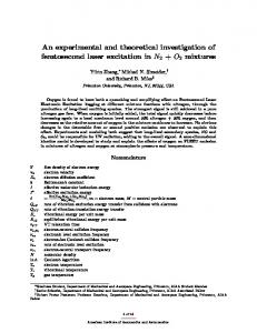
(a) CMA-ES Ackley (b) CMA-ES Griewank (c) CMA-ES Rastrigin Figure 3: Performance pk (mean solution quality CMA-ES achieved in 100 test runs using the method’s chosen parameter settings) of SPO 0.3, SPO 0.4, and SPO+ , as a function of the number of target algorithm runs, k, the method is allowed. We plot means of pk across 25 repetitions of each parameter optimisation procedure.

SPO 0.3 SPO 0.4 SPO+ p-value SPO 0.3 vs SPO 0.4 p-value SPO 0.3 vs SPO+ p-value SPO 0.4 vs SPO+

Sphere 10.3 × 10−7 ± 11.9 × 10−7 6.06 × 10−7 ± 8.88 × 10−7 5.56 × 10−7 ± 5.15 × 10−7 0.07 0.20 0.56

Ackley 9.34 ± 1.65 8.16 ± 1.48 8.48 ± 2.61 0.015 0.020 0.97

Griewank 453 × 10−4 ± 2140 × 10−4 1320 × 10−4 ± 6530 × 10−4 2.66 × 10−4 ± 2.53 × 10−4 0.95 0.00006 0.00009

Rastrigin 1130 ± 5653 4.06 ± 1.93 2.62 ± 0.51 1 0.0005 0.0014

Table 4: Comparison of different intensification mechanisms for optimising CMA-ES performance on a number of instances. We report mean ± standard deviation of performance p1000 (mean solution quality achieved by CMA-ES in 100 test runs using the parameter settings the method chose after 1000 algorithm runs) across 25 repetitions of each method, and p-values (see Sec. 2). “lucky” function evaluations, making them likely to become incumbents. In those runs, in almost every iteration a new incumbent was picked, because the previous incumbent had been found to be poor after performing additional runs on it. This situation continued throughout the entire parameter optimisation trajectory, leading to a final choice of parameter settings that had only been evaluated using very few (“lucky”) runs and performed poorly in independent test runs. This observation motivated us to introduce a different intensification mechanism that guarantees an increasing confidence in the performance of the parameter settings we select as incumbents. In particular, inspired by the mechanism used in FocusedILS [17], we maintain the invariant that we never choose an incumbent unless it is the parameter setting with the most function evaluations. Promising parameter settings receive additional function evaluations until they either cease to appear promising or receive enough function evaluations to become the new incumbent. In detail, our new intensification mechanism works as follows. In the first iteration, the incumbent is chosen exactly as in SPO, because all parameter settings have the same number of function evaluations. From then on, in each iteration we select a number of parameter settings and evaluate them as compared to the incumbent, θb∗ . Denote the number of runs with a parameter setting θ executed so far as N (θ) and their empirical performance as cˆ(θ). For each selected setting θ, we iteratively perform runs until either N (θ) ≥ N (θb∗ ) or cˆ(θ) > cˆ(θb∗ ).3 In the first case, if θ has reached as many runs as the incumbent, θb∗ , and cˆ(θ) ≤ cˆ(θb∗ ), then θ becomes the new incumbent. On the other hand, once cˆ(θ) becomes larger than cˆ(θb∗ ), we reject θ as (probably) inferior and perform as many additional runs for θb∗ as were just performed for evaluating θ; this mechanism ensures that we use a comparable number of runs for intensification and for exploration of new parameter settings. 3 In order to reduce the overhead arising from performing many algorithm runs one at a time, we batch runs, starting with a single new run for each θ and doubling the number of new runs iteratively up to a maximum of N (θb∗ ) − N (θ).

Note that the rejection is very aggressive and frequently occurs after a single run, long before a statistical test could conclude that θ is worse than θb∗ . The parameter settings we evaluate against θb∗ at each iteration include one new parameter setting selected based on an expected improvement criterion (here E[I 2 ], see Section 5.2). They also include p previously evaluated parameter settings θ1:p , where for each of these, a previously evaluated setting θ is selected with probability proportional to 1/ˆ c(θ) and repetitions are not allowed (p is an algorithm parameter and in this work always set to 5). This mechanism guarantees that there will always be a positive probability of re-evaluating a potentially optimal parameter setting; it allows us to be aggressive in rejecting new candidates, since we can always get back to the most promising ones. Note that if the other SPO variants (0.3 and 0.4) discover the optimal parameter setting but observe one or more very “unlucky” runs on it, there is a high chance that they will never recover: once a parameter setting has been evaluated, the noise-free Gaussian process model attributes zero uncertainty to it, such that no expected improvement criterion will pick it again in later iterations. We denote as SPO+ the variant of SPO that uses a random LHD, log-transformed data (for positive functions only; otherwise untransformed data), expected improvement criterion E[I 2 ] and our new intensification criterion. We compared SPO 0.3, SPO 0.4, and SPO+ (all based on a random LHD and log-transformed data) for our CMA-ES test cases and summarise the results in Table 4. For the Ackley function, SPO 0.4 performed best on average, but only insignificantly better than SPO+ ; for the Sphere function, SPO+ did insignificantly better than the other SPO variants. For the other two functions, SPO+ performed significantly and substantially better than either SPO 0.3 or SPO 0.4, finding parameter settings that led to CMA-ES performance orders of magnitude better than those obtained from SPO 0.3. More importantly, as can be seen in Figure 3, over the course of the optimisation process, SPO+ showed much less variation in the quality of the incumbent parameter setting than the other SPO variants. This is the case even for the Ackley function, where SPO+

5.2

Expected Improvement Criterion

In sequential model-based optimisation, parameter settings to be investigated are selected based on an expected improvement criterion (EIC). This aims to address the exploration/exploitation tradeoff faced in learning about new, unknown parts of the parameter space, and intensifying the search locally in the best known region. We briefly summarise two common versions of the EIC, and then describe a novel variation, which we investigated. The classic expected improvement criterion used by Jones et al. [19] is defined as follows. Given a deterministic function f , and the minimal value fmin seen so far, the improvement at a new design site θ is defined as I(θ) := max{0, fmin − f (θ)}.

(1)

Of course, this quantity cannot be computed, since f (θ) is unknown. We therefore compute the expected improvement, E[I(θ)]. To do so, we require a probabilistic model of f , in our case the Gaussian process model. Let µθ := E[f (θ)] be the mean, and σθ2 −µθ be the variance predicted by our model, and define u := fmin . σθ Then one can show that E[I(θ)] has the following closed-form expression: E[I(θ)] = σθ · [u · Φ(u) + ϕ(u)], (2) where ϕ and Φ denote the probability density function and cumulative distribution function of a standard normal distribution, respectively. A generalised expected improvement criterion was introduced by Schonlau et al. [23], who considered the quantity g

g

I (θ) := max{0, [fmin − f (θ)] }

(4)

One issue that seems to have been overlooked in previous work is the interaction of log transformations of the data with the EIC. When we use a log transformation, we do so in order to increase predictive accuracy, yet our loss function cares about the untransformed data (e.g., actual runtimes). Hence we should optimise the criterion Iexp (θ) := max{0, fmin − ef (θ) }. (5) Let v :=

ln(fmin )−µθ σθ

E[Iexp (θ)]

. Then one can show that 1

2

= fmin Φ(v) − e 2 σθ +µθ · Φ(v − σθ ).

(6)

+

In Table 5, we experimentally compare SPO with these three EI criteria on the CMA-ES test cases, based on a random LHD and log-transformed data. In one case, E[I 2 ] yielded the best results, and in three test cases our new criterion E[Iexp ] performed best. However, the overall impact of changing the expected improvement criterion was small and only two of the 12 pairwise differences were statistically significant.

5.3

Table 6: Comparison of final performance of various parameter optimisation procedures for optimising SAPS on instance QWH. We report mean ± standard deviation of performance p20000 (median search steps SAPS required on instance QWH in 1000 test runs using the parameter settings the method chose after 20 000 algorithm runs), across 25 repetitions of each method. Based on a Mann-Whitney U test, SPO+ performed significantly better than CALIBRA, BasicILS, FocusedILS, and SPO 0.3 with p-values 0.015, 0.0002, 0.0009, and 4×10−9 , respectively; the p-value for a comparison against SPO 0.4 was 0.06. 4

3

x 10

SPO 0.3 SPO 0.4 SPO+

2.5 2 1.5 1 0.5

3

10

(3)

for g ∈ {0, 1, 2, 3, . . .}, with larger g encouraging a more global search. The value g = 1 corresponds to the classic EIC. SPO uses g = 2, which takes into account the uncertainty in our estimate of I(θ) since E[I 2 (θ)] = (E[I(θ)])2 + Var(I(θ)) and can be computed by the closed form formula E[I 2 (θ)] = σθ2 · [(u2 + 1) · Φ(u) + u · ϕ(u)].

Procedure SAPS median run-time [search steps] SAPS default from [18] 85.5 × 103 CALIBRA(100) from [17] 10.7 × 103 ± 1.1 × 103 BasicILS(100) from [17] 10.9 × 103 ± 0.6 × 103 FocusedILS from [17] 10.6 × 103 ± 0.5 × 103 SPO 0.3 18.3 × 103 ± 13.7 × 103 SPO 0.4 10.4 × 103 ± 0.7 × 103 + SPO 10.0 × 103 ± 0.4 × 103

performance pk

did not perform best on average at the very end of its trajectory, and can also be seen on the Griewank and Rastrigin functions, where SPO+ clearly produced the best results.

Final Evaluation

In Sections 5.1 and 5.2, we fixed the design choices of using log transformations and initial designs based on random LHDs. Now, we revisit these choices: using our new SPO+ intensification criterion and expected improvement criterion E[I 2 ], we studied how

4

10 number of algorithm runs k

Figure 4: Comparison of SPO variants (all based on a random LHD and log-transformed data) for minimising SAPS median runtime on instance QWH. We plot the performance pk of each method (median search steps SAPS required on instance QWH in 1000 test runs using the parameter settings the method chose after k algorithm runs), as a function of the number of algorithm runs, k, it was allowed to perform; these values are averaged across 25 runs of each method. much the final performance of SPO+ changed when not using a log transform and when using different methods to create the initial design. Unsurprisingly, no initial design led to significantly better final performance than any of the others. The result for the log transform was more surprising: although we saw in Section 4 that the log transform consistently improved predictive model performance, based on a Mann-Whitney U test it only turned out to significantly improve final parameter optimisation performance for CMA-ES-sphere. As a final experiment, we compared the performance of SPO 0.3, 0.4, and SPO+ (all based on random LHDs and using logtransformed data) to the parameter optimisation methods studied by Hutter et al. [17]. We summarise the results in Table 6. While SPO 0.3 performed worse than those methods, SPO 0.4 performed comparably, and SPO+ outperformed all methods with the exception of SPO 0.4 significantly. Figure 4 illustrates the difference between SPO 0.3, SPO 0.4, and SPO+ for this SAPS benchmark. Similar to what we observed for CMA-ES (Figure 3), SPO 0.3 and SPO 0.4 changed their incumbents very frequently, with SPO 0.4 showing more robust behaviour than SPO 0.3, and SPO+ in turn much more robust behaviour than SPO 0.4.

E[I] from [19] E[I 2 ] from [23] E[Iexp ] (new) p-value E[I] vs E[I 2 ] p-value E[I] vs E[Iexp ] p-value E[I 2 ] vs E[Iexp ]

Sphere 8.60 × 10−7 ± 1.03 × 10−7 5.56 × 10−7 ± 5.15 × 10−7 8.01 × 10−7 ± 12.90 × 10−7 0.29 0.63 0.54

Ackley 8.36 ± 2.65 8.48 ± 2.61 8.30 ± 2.65 0.55 0.25 0.32

Griewank 3.51 × 10−4 ± 3.06 × 10−4 2.66 × 10−4 ± 2.53 × 10−4 2.48 × 10−4 ± 2.51 × 10−4 0.016 0.11 0.77

Rastrigin 2.66 ± 0.57 2.62 ± 0.51 2.56 ± 0.66 0.90 0.030 0.38

Table 5: Comparison of different expected improvement criteria for optimising CMA-ES performance on a number of functions. We report mean ± standard deviation of performance p1000 (mean solution quality CMA-ES achieved in 100 test runs using the parameter settings the method chose after 1 000 algorithm runs) of SPO 0.3, SPO 0.4, and SPO+ , across 25 repetitions of each method, and p-values as discussed in Section 2.

6.

CONCLUSIONS AND FUTURE WORK

In this work, we experimentally investigated model-based approaches for optimising the performance of parameterised, randomised algorithms. We restricted our attention to procedures based on Gaussian process models, the most widely-studied family of models for this problem. We evaluated two approaches from the literature, and found that sequential parameter optimisation (SPO) [4] offered more robust performance than the sequential kriging optimisation (SKO) approach [15]. We then investigated key design decisions within the SPO paradigm, namely the initial design, whether to fit models to raw or log-transformed data, the expected improvement criterion, and the intensification criterion. Out of these four, the log-transformation and the intensification criterion substantially affected performance. Based on our findings, we proposed a new version of SPO, dubbed SPO+ , which yielded substantially better performance than SPO for optimising the solution quality of CMA-ES [14, 13] on a number of test functions, as well as the run-time of SAPS [18] on a SAT instance. In this latter domain, for which performance results for other (model-free) parameter optimisation approaches are available, we demonstrated that SPO+ achieved state-of-the-art performance. In the future, we plan to extend our work to deal with optimisation of runtime across a set of instances, along the lines of the approach of Williams et al. [25]. We also plan to compare other types of models, such as random forests [10], to the Gaussian process approach. Finally, we plan to develop methods for the sequential optimisation of categorical variables. Acknowledgements. We thank Thomas Bartz-Beielstein for providing the SPO source code and an interface to the CMA-ES algorithm online, and Theodore Allen for making the original SKO code available to us.

7.

REFERENCES

[1] B. Adenso-Diaz and M. Laguna. Fine-tuning of algorithms using fractional experimental design and local search. Operations Research, 54(1):99–114, Jan–Feb 2006. [2] C. Audet and D. Orban. Finding optimal algorithmic parameters using the mesh adaptive direct search algorithm,. SIAM Journal on Optimization, 17(3):642–664, 2006. [3] P. Balaprakash, M. Birattari, and T. Stützle. Improvement strategies for the f-race algorithm: Sampling design and iterative refinement. In T. Bartz-Beielstein, M. J. Blesa Aguilera, C. Blum, B. Naujoks, A. Roli, G. Rudolph, and M. Sampels, editors, 4th International Workshop on Hybrid Metaheuristics (MH’07), pages 108–122, 2007. [4] T. Bartz-Beielstein. Experimental Research in Evolutionary Computation: The New Experimentalism. Springer Verlag, 2006. [5] T. Bartz-Beielstein, C. Lasarczyk, and M. Preuss. Sequential parameter optimization. In B. McKay et al, editor, Proc. of CEC-05, pages 773–780. IEEE Press, 2005. [6] T. Bartz-Beielstein, C. Lasarczyk, and M. Preuss. Sequential parameter optimization toolbox. Manual version 0.5, September 2008, available at http://www.gm.fh-koeln.de/imperia/ md/content/personen/lehrende/bartz_beielstein_thomas/ spotdoc.pdf, 2008.

[7] T. Bartz-Beielstein and M. Preuss. Considerations of budget allocation for sequential parameter optimization (SPO). In L. Paquete et al., editor, Proc. of EMAA-06, pages 35–40, 2006. [8] B. Beachkofski and R. Grandhi. Improved distributed hypercube sampling. American Institute of Aeronautics and Astronautics Paper 2002-1274, 2002. [9] M. Birattari, T. Stützle, L. Paquete, and K. Varrentrapp. A racing algorithm for configuring metaheuristics. In Proc. of GECCO-02, pages 11–18, 2002. [10] L. Breiman. Random forests. Machine Learning, 45(1):5–32, 2001. [11] S. P. Coy, B. L. Golden, G. C. Runger, and E. A. Wasil. Using experimental design to find effective parameter settings for heuristics. Journal of Heuristics, 7(1):77–97, 2001. [12] N. Hansen. The CMA evolution strategy: a comparing review. In J.A. Lozano, P. Larranaga, I. Inza, and E. Bengoetxea, editors, Towards a new evolutionary computation. Advances on estimation of distribution algorithms, pages 75–102. Springer, 2006. [13] N. Hansen and S. Kern. Evaluating the CMA evolution strategy on multimodal test functions. In X. Yao et al., editors, Parallel Problem Solving from Nature PPSN VIII, volume 3242 of LNCS, pages 282–291. Springer, 2004. [14] N. Hansen and A. Ostermeier. Adapting arbitrary normal mutation distributions in evolution strategies: the covariance matrix adaptation. In Proc. of CEC-96, pages 312–317. Morgan Kaufmann, 1996. [15] D. Huang, T. T. Allen, W. I. Notz, and N. Zeng. Global optimization of stochastic black-box systems via sequential kriging meta-models. Journal of Global Optimization, 34(3):441–466, 2006. [16] F. Hutter, H. Hoos, K. Leyton-Brown, and T. Stützle. ParamILS: An automatic algorithm configuration framework. Technical Report TR-2009-01, University of British Columbia, January 2009. [17] F. Hutter, H. H. Hoos, and T. Stützle. Automatic algorithm configuration based on local search. In Proc. of AAAI-07, pages 1152–1157, 2007. [18] F. Hutter, D. A. D. Tompkins, and H. H. Hoos. Scaling and probabilistic smoothing: Efficient dynamic local search for SAT. In Proc. of CP-02, pages 233–248, 2002. [19] D. R. Jones, M. Schonlau, and W. J. Welch. Efficient global optimization of expensive black box functions. Journal of Global Optimization, 13:455–492, 1998. [20] K. Leyton-Brown, E. Nudelman, and Y. Shoham. Learning the empirical hardness of optimization problems: The case of combinatorial auctions. In Proc. of CP-02, 2002. [21] J. Sacks, W. J. Welch, T. J. Welch, and H. P. Wynn. Design and analysis of computer experiments. Statistical Science, 4(4):409–423, November 1989. [22] T. J. Santner, B. J. Williams, and W. I. Notz. The Design and Analysis of Computer Experiments. Springer Verlag, New York, 2003. [23] M. Schonlau, W. J. Welch, and D. R. Jones. Global versus local search in constrained optimization of computer models. In N. Flournoy, W.F. Rosenberger, and W.K. Wong, editors, New Developments and Applications in Experimental Design, volume 34, pages 11–25. Institute of Mathematical Statistics, Hayward, California, 1998. [24] D. A. D. Tompkins and H. H. Hoos. Ubcsat: An implementation and experimentation environment for SLS algorithms for SAT & MAX-SAT. In Proc. of SAT-04, 2004. [25] B. J. Williams, T. J. Santner, and W. I. Notz. Sequential design of computer experiments to minimize integrated response functions. Statistica Sinica, 10:1133–1152, 2000.