The Hough Transform (HT) is a commonly used method for line detection that is successfully applied in a large range of vision problems, starting from specific ...
Proceedings of the Croatian Computer Vision Workshop, Year 3
September 22, 2015, Zagreb, Croatia
An Extension to Hough Transform Based on Gradient Orientation Tomislav Petkovi´c and Sven Lonˇcari´c University of Zagreb Faculty of Electrical and Computer Engineering Unska 3, HR-10000 Zagreb, Croatia Email: {tomislav.petkovic.jr, sven.loncaric}@fer.hr
Abstract—The Hough transform is one of the most common methods for line detection. In this paper we propose a novel extension of the regular Hough transform. The proposed extension combines the extension of the accumulator space and the local gradient orientation resulting in clutter reduction and yielding more prominent peaks, thus enabling better line identification. We demonstrate benefits in applications such as visual quality inspection and rectangle detection. Index Terms—Hough transform, gradient orientation
I. I NTRODUCTION The Hough Transform (HT) is a commonly used method for line detection that is successfully applied in a large range of vision problems, starting from specific applications in industrial and robotic vision and extending to a general unconstrained problem of line detection in natural images. The success of the HT is primarily based on recasting a complex global line detection problem into a simple task of finding local peaks (concentrations of votes) in some parameter space. The HT was proposed by Paul V. C. Hough [1] in 1962 and was introduced to computer vision community by Duda and Hart [2]. A comprehensive review of the HT was given by Illingworth and Kittler [3] in 1989. Later research introduced a randomized Hough transform (RHT) and its variants [4], [5], [6], [7] that eliminate the need for the quantized parameter space. Other improvements include better and more robust peak detection [8], [9] and extraction of line length [10], [11], [8]. Most of the above mentioned HT variants use only coordinates of extracted edge points and disregard other data that is often extracted from the input image during the edge or ridge detection. In this paper we propose to improve upon a HT extension first suggested by O’Gorman and Clowes [12] that uses the gradient orientation to place a limit on the range of line orientation θ in the (θ, ρ) parameter space; if the detected gradient orientation is θ0 then votes are only accumulated for the predetermined range ∆θ around the θ0 , the interval hθ0 −∆θ, θ0 +∆θi. We extend this approach by combining the gradient orientation with the extension of accumulator space that makes straight line parametrization non-unique, but, combined with the range limit on orientation θ, offers advantages of further clutter reduction and yields more prominent peaks. The paper is organized as follows: In Section II a brief review of HT is given. In Section III a proposed accumulator
CCVW 2015 Feature Extraction
array extension is introduced. In Section IV some results are presented and discussed. We conclude in Section V. II. T HE H OUGH T RANSFORM Hesse normal form of a straight line is ~r · n ˆ − ρ = 0,
(1)
where ~r = ~ıx + ~y is the location vector of the point (x, y), n ˆ = ~ı cos θ + ~ sin θ is the unit normal vector of the straight line and ρ ≥ 0 is the distance to the origin. For the HT Eq. (1) is usually rewritten as ρ = x cos(θ) + y sin(θ),
(2)
which defines a sinusoid in (θ, ρ) parameter space that corresponds to a point (x, y) in the input image. For the HT a sinusoid defined by Eq. (2) is drawn in the parameter space for every edge point (x, y). Straight lines present in the input image are given by (θ, ρ) coordinates of the local peaks in the parameter space. The parameters θ and ρ are usually limited to either [− π2 , π2 ] × h−∞, +∞i or [−π, π] × [0, +∞i intervals, i.e. to ranges that produce unique mapping. For real world images ±∞ limit of parameter ρ is replaced by ρmax defined by the finite size of the image. Points (x, y) are selected by an edge detector, most often by thresholding a gradient of the input image. Therefore, in addition to point coordinates, the direction and magnitude of the gradient are also known. Let gx and gy be components of the gradient in x and y directions. The gradient direction vector is perpendicular to the local edge so, as shown in [12], the orientation θ can be estimated as gy (3) θ ≈ atan , gx and all sinusoids in (θ, ρ) space may be drawn only for a small interval of angles centered around the estimate of Eq. (3), thus reducing the clutter. III. P ROPOSED ACCUMULATOR E XTENSION We propose to extend the accumulator so θ ∈ [−π, π] and ρ ∈ [−ρmax , ρmax ], where ρmax is determined by the size of the input image. This extension makes the straight line parametrization in (θ, ρ) space non-unique: every straight line
15
Proceedings of the Croatian Computer Vision Workshop, Year 3
0 −ˆ n
y=
− 43 x
September 22, 2015, Zagreb, Croatia
x +3
n ˆ
(b) ROI
y Fig. 1: A straight line y = − 43 x + 3 with two unit normals in opposite directions. (a) Annotated QC image
(−126.9◦ , −2.4)
π
−π ρ
Fig. 3: QC example: Positioning of a flat spring in regard to a bearing structure must be examined. (a) is annotated QC image showing measures of interest. (b) shows a ROI. (c) shows found boundary lines delineating a flat spring.
θ
(53.1◦ , 2.4)
Fig. 2: HT of a point (1.44, 1.92) on a line y = − 34 x + 3.
in the image is represented by two different points in the proposed accumulator range. However, those two representations have exactly opposite normal directions. For example, consider the line y = − 43 x + 3 shown in Fig. 1; two unit normals are n ˆ , pointing away from the origin, and −ˆ n, pointing toward the origin. The normal n ˆ corresponds to the equation 12 3 4 n corresponds 5 = 5 x + 5 y, while the opposite normal −ˆ 3 4 = − x − y, which defines the same to the equation − 12 5 5 5 straight line. The HT of the point (1.44, 1.92) closest to the origin marked with dot in Fig. 1 is shown in Fig. 2; two dots in Fig. 2 correspond to two possible directions of the straight line normal. However, the parametrization in proposed extended accumulator becomes unique if the notion of line direction is introduced; let the line direction vector dˆ be defined so n ˆ and dˆ form a right-hand coordinate system. Therefore, instead of straight lines we are detecting oriented straight lines. The proposed extension depends on the gradient orientation. Let gx and gy be components of the gradient at (x, y). The orientation θ for point at (x, y) can be estimated as θ ≈ atan2(gy , gx ),
(4)
so the atan function of Eq. (3) yielding angles in the [− π2 , π2 ] interval is replaced by atan2 that yields angles in the [−π, π] interval. The sinusoid in (θ, ρ) space is drawn only for a small interval of angles centered around the orientation estimate of Eq. (4), however, due to additional separation of points with opposing gradients we expect further clutter reduction in the HT domain. Examining again the Fig. 2 demonstrates the difference: the plain HT would increment the accumulator array for all points on a sinusoid over θ ∈ [− π2 , π2 ] range, the HT using the gradient direction to limit the angle range would increment the accumulator on the segment around (53.1◦ , 2.4) point, and the
CCVW 2015 Feature Extraction
(c) Found lines
proposed method would increment the accumulator on either segment around (53.1◦ , 2.4) or around (−126, 9◦ , −2.4) point, depending on the gradient orientation. IV. R ESULTS AND D ISCUSSION In this Section we present several examples demonstrating the advantages of the proposed extension to the HT. For all input images the coordinate axes are as shown in Fig. 1 with the origin in the center. For all accumulator arrays the coordinate axes are as shown in Fig. 2 with the origin in the center. Values of accumulator arrays are mapped through a square root function, linearly scaled to available dynamic range and inverted; pure black corresponds to the highest accumulator value, white is zero, and mid-levels are gray. Such mapping compresses the dynamic range, reduces the intensities of peaks, and makes butterfly shapes around peaks clearly visible. Line distance to origin ρ is measured in pixels and orientation θ in degrees. Range ∆θ around θ0 was set to 22.5◦ . A. Visual Quality Control The HT is often applied in industrial vision tasks. We give two examples in visual quality control (QC) where a thin structure must be delineated. The first example is QC of a thin flat spring whose position against the bearing structure must be inspected. An example is shown in Fig. 3: the input image is annotated showing structures of interest. The accumulator arrays for the regular HT and for the proposed HT are shown in Fig. 4: note the increased separation of two peaks that correspond to the upper and lower straight lines that delineate the thin flat spring. This separation effect is caused by the proposed accumulator extension and the use of the extracted gradient orientation; it will reduce clutter in the accumulator when spatially close features in the input image have different gradient orientations. The second example demonstrates a more difficult visual QC task where position and inclination angles of a thin flat spring must be inspected. The flat spring is about one pixel thin, which is the main difficulty. The input image and steps of
16
Proceedings of the Croatian Computer Vision Workshop, Year 3
September 22, 2015, Zagreb, Croatia
θ = 85.0◦ , ρ = 24.9 (merged)
θ = 47◦ , ρ = −48 θ = 47◦ , ρ = −20 θ = 47◦ , ρ = −20 θ = −133◦ , ρ = 49
(a) Accumulator array for regular HT where − π2 < θ