An Implementation-Oriented Semantics for Module Composition

An Implementation-Oriented Semantics for Module Composition Joseph A. Goguen

Department of Computer Science & Engineering University of California at San Diego La Jolla CA 92093-0114

Will Tracz

Lockheed Martin Federal Systems Owego, New York 13827-3994

Abstract: This paper describes an approach to module composition by executing \module expressions" to build systems out of component modules. This approach extends the structural description capabilities of existing Architecture Description Languages (ADLs) to facilitate the manipulation of architectural components in a manner that results in either new components or complete instantiations of parameterized architectures. The paper also gives a novel semantics intended to aid with the implementation this approach. The semantics is based on set theory, and uses the technical notions of tuple set, partial signature, and institution, avoiding more dicult mathematics such as abstract algebra and category theory. Language features include information hiding, both vertical and horizontal composition, and views for binding modules to interfaces. Vertical composition refers to the hierarchical structuring of a system into layers, while horizontal composition refers to the structure of a given layer. Modules may involve information hiding, and views may involve behavioral satisfaction of a theory by a module. Finally, this paper includes a number of \Laws of Software Composition" that show how the various module composition operations are related.

1 Introduction

No way of thinking or doing, however ancient, can be trusted without proof. | Henry David Thoreau, \Economy," Walden (1854).

The approach to module composition described in this paper can be used for many dierent programming languages, by providing a simple module connection language (MCL) with \module expressions" that say how to manipulate and connect modules in the programming language. The general approach, called \parameterized programming" [10], involves a module speci cation capability; however, programmers can specify as little of a module as they like, as long as they declare the syntax. The approach has been validated with experiments using lileanna [40] on real examples. lileanna, which has Ada [6] as its implementation language and Anna [27, 29] as its speci cation language, is also used for illustrations in this paper. Furthermore, this approach extends the structural description capabilities of existing Architecture Description Languages (ADLs) (e.g., [30, 8] to facilitate the manipulation of architectural components in a manner that results in either new components or complete instantiations of parameterized architectures. Our semantics for module expressions uses simple set theoretic manipulations to de ne module composition operations. This semantics is intended to aid implementors of module composition facilities; hence it is not a denotational or axiomatic semantics in the usual sense. In particular, it does not directly address the semantics of statements or what happens at compile time or at run time; instead, it is concerned with the semantics of modules and their interconnection, i.e., with what happens at module composition time. For this reason, it abstracts away details of the languages used for speci cation and programming.  This research was supported in part by the Defense Advanced Research Projects Agency (DARPA) in cooperation with the US Air Force Wright Laboratory Avionics Directorate under contract # F33615-91-C-1788, the European Community under ESPRIT-2 BRA Working Groups 6071, IS-CORE (Information Systems COrrectness and REusability) and 6112, COMPASS (COMPrehensive Algebraic Approach to System Speci cation and development), Fujitsu Laboratories Limited, and the Information Technology Promotion Agency, Japan, as part of the R & D of Basic Technology for Future Industries \New Models for Software Architecture" project sponsored by NEDO (New Energy and Industrial Technology Development Organization).

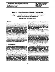
Module composition languages can be used at least two dierent ways in software development: 1. descriptively, to specify and analyze a given design or architecture (i.e., the interfaces and interconnections of modules); and 2. constructively, to create a new design from existing modules, using operations that combine and transform modules. Using an MCL descriptively is like writing and reading a blueprint; it tells you about the structure of a house; languages that only provide these capabilities are often called MILs1 , Module Interconnection Languages [35]. Using an MCL constructively is like having robots build a (modular) house by following the blueprint. This facilitates reuse and helps support controlled evolution. As illustrated in Figure 1, it can simplify the software lifecycle by eliminating detailed design and coding2 , provided a suitable library of software modules with their speci cations and interrelationships is available. Parameterized programming supports this by executing module expressions, and thus goes far beyond merely specifying modules and systems.

r r Speci cation r Detailed Design r r r

Code

Module Composition

6

r

r

Test

r

Figure 1: Idealized Software Lifecycle with and without Module Composition

Analogy with Functional Programming It may be helpful to think of module composition as functional programming with modules (see [2] for a nice exposition of this idea). The analogy is appropriate because there is no state at module composition time. Instead, we are evaluating expressions, called module expressions, that say how to put together software components. The result of evaluating a module expression is a value, namely the composed system; it is built by applying module composition operations to subsystems, which are also values. Under this analogy, modules have types that are called theories. A theory is another kind of module that is used to describe both the syntax and semantics of modules that supply code. We write C :: T to indicate that a module C has the \large grain type" T; this involves more than the usual notion of type indicated by the notation C : T, because (what we call) a view must be given from T to C, binding the formal symbols in T to actual symbols in C. Furthermore, the axioms in T should be satis ed by the corresponding implementations of the symbols in C. Views are also used in instantiating parameterized modules, to say how to bind symbols of a parameterized module's interface theory to symbols (e.g., types and operators) in the module used as an actual parameter. The axioms in the theory of a module give rise to \proof obligations;" these are mathematical assertions that should be true in order for the program to work as expected. We do not recommend that the proof aspect of this notion of type should be required for normal production programming, but rather that a \hook" should be left, in case rigorous formal methods are required for some critical application. Thus in normal programming, the axioms 1 It is interesting to note that much of the basic language constructs in MILs have served as that basis for the structural description capabilities in current ADLs. 2 This gure is itself a great oversimpli cation, because it omits the processes of feedback and reconstruction that occur in real software development projects. Research on the sociology of software development shows that the division of tasks into phases is to a large extent arbitrary, and is also subject to reclassi cation as the project evolves; see papers in [26], especially [5] and [15], and also see [16].

2

serve to document properties of interfaces the designers and programmers considered especially important, and believed to be true, perhaps as the result of informal reasoning. The word \type" has many dierent meanings in computer science. There are the \small grain types" used in speci cation and programming languages; in our examples, these will be lileanna and Ada types. There are also the \large grain types" described above. Moreover, the word \type" is used in a branch of logic called \type theory" for syntactic expressions (that may include axioms) for describing collections of entities. Types in the type theory sense cannot handle modules in our sense very smoothly, because small grain types and operators can only be encapsulated together through an awkward encoding into a single complicated type. There are two kinds of type in lileanna: (1) purely syntactic types that correspond to those in a programming language, and (2) types in roughly the sense of type theory, i.e., programming language types and operations encapsulated together with some axioms, which are used to de ne semantic subtypes of the programming and speci cation language types. Hereafter this paper will in general only use the word \type" for programming language types, and will use the word \theory" for the large grain type used for modules3.

Some History The paradigm for module composition described in this paper is based on parameterized pro-

gramming and hyperprogramming4 [10, 12]. Because this approach involves modules for both speci cation and code, both kinds of module must be composed. Speci cations are used as \headers" for code, and are combined with simple set theoretic operations. At the code level, composition may be done with intermediate compiled code, which is then sent to the compiler backend after composition has been completed. In the case of lileanna with Ada, this means using diana5 [38, 39]. Although we avoid complex mathematics, such as abstract algebra and category theory, both the module composition facility and its semantics as described in this paper are largely inspired by work done using such formalisms, including the Clear speci cation language [3, 4], and the OBJ [21, 25] system. The approach in this paper diers from that of those languages in providing a constructive module composition facility for an imperative programming language. This was contemplated for the CAT [17] and LIL [9] systems, which are the closest ancestors of the approach in this paper; however, details of the semantics of these systems were not fully developed and they were not implemented. This paper also presents some extensions to the original conception of parameterized programming. The set theoretic implementation oriented semantics in this paper is novel. Sannella [36] gave a pioneering set theoretic semantics for Clear. The elegant work of Wirsing [42] on the ASL kernel speci cation language also involved a set theoretic approach. Moreover, many papers have used institutions and category theory to achieve generality (e.g., see [4, 7, 37] and [13]). However, it has seemed that the generality of institutions was incompatible with the speci city of set theory, and this is the rst paper to combine these two approaches, as well as the rst to use tuple sets and partial signatures. The work in this paper also diers from most previous work in the algebraic speci cation tradition in that it is concerned with generating systems, rather than just specifying them, i.e., it is constructive as well as descriptive. Another unusual feature is the use of information hiding in speci cations and the resulting behavioral (i.e., \black box") notion of satisfaction for views [22, 20]). The version of parameterized programming in this paper, like that in LIL, provides both horizontal and vertical composition. Vertical composition concerns the structuring of a system into layers, each providing services to higher layers, while horizontal composition concerns the structure of each layer. Some basic laws for composing speci cations were proved in [23] and also in [37]. 3 The parameterized programming literature [10] uses the word \sort" for small grain types, and we may occasionally use this

terminology if extra clarity is needed. 4 The term megaprogramming has more recently been used for these ideas within the DARPA community [1, 41]. 5 This is an acronym for Descriptive Intermediate Attributed Notation for Ada.

3

1.1 Summary of the Paper There are two main technical ideas that make the goals of this paper feasible: (1) tuple sets, which allow simple recursive de nitions of basic set theoretic operations like union and inclusion for complex structures like signatures and speci cations, and (2) institutions, which axiomatize the intuitive notion of logical system. Tuple sets are introduced in Section 2.2; they permit simpli ed de nitions of operations for combining modules, based on set theory. They also permit us to de ne the notion of partial signature, which again simpli es our de nitions. Institutions, introduced in Section 2.3, let us handle both speci cation and programming languages while avoiding the enormous complexity of their semantic de nitions. Horizontal composition is discussed in Section 4, beginning with a discussion of the module graph in Section 2.1. This is the basic data structure for our semantics; its nodes are module names, and its edges indicate relationships between modules, including inheritance. Each module name M has associated to it a speci cation module Q(M ), and a list I (M ) of implementation modules. The main mechanisms for horizontal composition are renaming, aggregation, and instantiation of generic modules. These are discussed in Sections 3.3, 4.4, and 4.6, respectively; views are discussed in Section 3.3. The notion of view introduced there diers from previous notions in that it respects information hiding, i.e., it only requires behavioral satisfaction of axioms; it also takes account of imported modules. Overload resolution is discussed in Section 3.1.1 and a way of adding or removing functionality from modules is discussed in Section 4.6. Module expressions are discussed in Section 4.7. Vertical composition, as discussed in Section 5, allows designs to have multiple layers, where each layer provides services to higher layers. Furthermore, each layer may itself have a complex horizontal structure, involving the composition of multiple modules. The module system provided by parameterized programming is much more powerful than that of Ada, and in fact it provides all of the power of higher order programming without the need for higher order functions, as shown in [11]. This paper includes a number of \Laws of Software Composition," which say how various composition operations are related to one another. These are useful in implementing a module composition system, and many have never appeared before, especially those involving vertical composition.

1.2 Conventions for Exposition De nitions, examples, results (theorems, propositions, corollaries, etc.) are numbered sequentially on a single \counter." Thus, Example 4 follows De nition 3, and there is no De nition 4. This method of enumeration is intended to facilitate browsing. Assumptions and laws each have their own environment, and are numbered separately. Assumptions are gradually enriched with further conditions, in the hope that many readers will nd the paper easier to follow this way. We may abbreviate \if and only if" by \i". If S is a set, then S  denotes the set of all nite lists from S , including the empty list, which is denoted []. We denote a list with n elements using the notation [a1 ; :::; a ]. n

2 Foundational Concepts

Let all laws be clear, uniform, and precise; to interpret laws is almost always to corrupt them. | Francois Voltaire, Philosophical Dictionary (1764).

This section discusses some concepts that provide the mathematical foundation for the development that follows. These are: (1) the module graph; (2) the notions of tuple set and signature; (3) the notions of sentence and model; and (4) the notion of institution, which ties together the notions of signature, sentence and model. These concepts are necessarily rather abstract, because of our goal of treating any (suitable) combination of programming and speci cation language. 4

2.1 The Module Graph The parts from which systems are constructed are called modules. Parameterized programming has two kinds of module: (1) speci cation modules, and (2) implementation modules, which are discussed in Sections 3.1 and 3.2, respectively. The following gives a rst de nition for the basic module graph data structure that is assumed throughout this paper. It is gradually extended with further assumptions to handle further features of parameterized programming as they are introduced.

De nition 1 A module graph G consists of a nite set N of nodes, called module names, a nite set E of edges, two functions, d0 ; d1 : E ! N , which respectively give the source and target node for each edge, plus an acyclic subgraph H, called the inheritance graph, having the same node set N as G; thus, the edges of H, called inheritance edges, are a subset I of E , and the source and target functions of H agree with d0 and d1 on I . We write N < M if there is a path from N to M in H. We may use the notation e : M ! M 0 to indicate that e is an edge with d0 (e) = M and d1 (e) = M 0 . 2

Intuitively, the edges of the module graph indicate relationships between modules, of which the most basic are those of inheritance, indicated by the edges in the inheritance subgraph6. N < M means that M inherits from N . This relation is transitive because the composition of two paths is another path. (The idea of module graphs may be found in [14].) Another kind of relationship between modules, indicated by edges in the module graph, is given by a view, which asserts that the target module satis es the axioms given in the source module; views are discussed in Section 3.3. The module graph G describes the resources available at a given moment for building systems, including both modules and knowledge about their properties; the role of G is analogous to that of an environment for evaluating expressions in a programming language.

Assumption 1 There is a xed module graph G, with a xed inheritance subgraph H. 2 Example 2 Assume modules M 1; M 2; M 3 such that module M 3 inherits M 2 and module M 2 inherits M 1, i.e., M 1 < M 2 < M 3. Then the module graph G has three nodes, named M1; M2 and M3, and two edges, one from M1 to M2 , and one from M2 to M3, as shown in Figure 2. Both edges are inheritance edges. 2

# "M

1

# inherits ! "M

2

# inherits ! "M

Figure 2: A Simple Module Graph

3

!

As we will see later, other information can also be associated with a module name, such as a description of the data representations used, test cases, and administrative information (e.g., the history of various implementations, such as programmer, date, and comments). All this is important for handling the evolutionary aspects of software development.

2.2 Signatures and Tuple Sets We will later assume that there is a given xed class Sign of signatures, which are used for declaring the syntax of modules, such that all signatures are tuple sets, in the sense of De nition 3 below. In this recursive de nition, 6 Instead of having a subgraph H of G, we could put the label \inherits" on all inheritance edges, as suggested by Figure 2.

5

(0) is the base case and (1) is the recursive step. It may help the reader to visualize tuple sets as ordered trees that have sets on their leaf nodes.

De nition 3 A tuple set is either

(0) a set, or else (1) a tuple of tuple sets. Two tuple sets have the same form if and only if they are both sets, or else are tuples of the same length such that their corresponding components have the same form. More formally, t  t0 i (0) t and t0 are both sets, or else (1) t and t0 are tuples of the same length, say n, and t  t0 for i = 1; :::; n. i

i

We will use the notation (t1 ; :::; t ) for a tuple having n components, called an n-tuple. The sets that occur as the bottom level components of a tuple set are called its base sets, and their elements are called its symbols. n

2

Figure 3 shows a typical tuple set structure, where the circles represent the base sets of symbols, and the internal nodes represent tuples. Sometimes we want to use pairs, triples, lists, etc. that are not tuples. For these cases, we will use the notation [t1 ; :::; t ] for a list of length n, and call it a pair when n = 2 and a triple when n = 3. n

r r jjj r r r jjj j j ?@ ? ?@ @?@ @@ ?@? ?? @ ??@@

Figure 3: A Tuple Set Structure

Example 4 Any set S is a tuple set. Also, any tuple of sets is a tuple set, e.g., (fa; bg; f1; 2g). Similarly, any tuple of tuple sets is a tuple set, e.g., (fa; b; cg; (fa; bg; f1; 2g)). And so on recursively. The tuple set (fa; b; cg; (fa; bg; f1; 2g)) has symbols a; b; c; 1; 2. On the other hand, the tuple set f[0; 0]; [?; 1]g has as its symbols the lists [0; 0] and [?; 1], rather than 0; 1, and ?. 2 (Although we want to avoid being distracted by problems in the foundations of mathematics in this paper, we also want to be consistent with the usual set theoretic foundations. Therefore we want everything to be a set, including our tuples and our tuple sets. To this end, we may distinguish between sets as used in De nition 3 (these are the circles in Figure 3) and sets in the sense of set theory, by calling the former \set"s and the latter just \set"s. Then tuples should be \set"s but not \set"s. This can be achieved in various ways. One is to use special ground elements (also called \urelements") to index the components of tuples, and never use those urelements for anything else; then everything is a \set", but only those \set"s that have not been formed using tuples (i.e., using the special urelements) are \set"s. Another approach is to give an axiomatization for set theory with a special constructor for tuples in addition to the usual ones for power set, etc. A third approach is to de ne tuple sets as the abstract data type of ordered trees with leaf nodes labeled by sets.)

The ordered tree view of tuple sets shows that we can use paths as selectors for the base sets of tuple sets. If  is a tuple set and p is a path to a leaf node, then we let  denote the base set that is attached to that leaf node. p

6

Example 5 The various signatures used for equational logic are tuple sets. For unsorted equational logic, there is a set O of operator symbols, plus an assignment of an arity7 a(o) to each o 2 O. Since a is a function, it can of course be viewed as a set of pairs in the usual way. Thus, we have  = (O; a) where a is a set of pairs [o; n] where n is a non-negative integer and o 2 O, such that there is exactly one such pair for each o 2 O. Alternatively, we could let  be a set of pairs [o; n], where n is a natural number giving the arity8 ; we can then de ne O from , as the set of all o's that occur in the pairs in . Notice that this second approach allows overloading, in that the same operator symbol o can occur with more than one arity n. (Note that the pairs [o; n] are not tuple sets here, they are symbols.) For many sorted (also called \heterogeneous") equational logic, signatures consist of a set S of sorts (i.e., \types") plus a set  of operator symbols of sort s and arity w, for each s 2 S and w 2 S  . Thus, a signature is a pair (S; r) where S is a set and r is a set of triples [w; s; o] with s 2 S , w 2 S  , and o an operator symbol. This formulation again allows overloading, in that a given operator symbol o can occur with more than one \rank" [w; s]. 2 w;s

We can de ne relations and operations on tuple sets like equality, inclusion, union, intersection, product and dierence, component-wise, by recursion over the tuple set structure:

De nition 6 Two tuple sets, t; t0 are equal, written t = t0, i they have the same form and all their correspond-

ing components are equal, i.e., if and only if t and t0 have the same number of components, say n, and t = t0 for i = 1; :::; n. We de ne inclusion similarly: t  t0 i t and t0 have the same form, with say n components, and t  t0 for i = 1; :::; n. Finally, the dierence (or the union) of two or more tuple sets, all of the same form, is formed by taking the dierence (or union) of the tuple sets occurring as their components. 2 i

i

i

i

Because signatures are tuple sets, De nition 6 gives us a natural notion of subsignature:  is a subsignature of 0 i   0 as tuple sets. For example, we have (H; (T; O; V; E ); (T ; O ; V ; E ); A)  (H 0 ; (T 0 ; O0 ; V 0 ; E 0 ); (T 0 ; O0 ; V 0 ; E 0 ); A0 ) X

X

X

X

X

X

X

X

if and only if H  H 0 and T  T 0 and O  O0 and so on. The assumption that signatures are tuple sets also gives us a natural notion of signature map. Here, we de ne it as a special case of the (also natural) notion of a relation between two tuple sets of the same form, as a tuple set again having the same form, and having pairs of symbols as its own symbols.

De nition 7 Given tuple sets ; 0 of the same form, then a tuple set relation  ! 0 is a tuple set9 of pairs of symbols (i.e., a subset of   0 ). A tuple set relation is a tuple set map i each of its base sets is a relation that is actually a function. A tuple set map is injective or surjective i each of its base set functions is. Similarly, a tuple set map is an isomorphism i each of its base set functions is; in this case we may write   0 . Given a tuple set and a tuple set relation h : ! , let  h be the tuple set with each symbol a in each base set B of replaced by the corresponding symbols a0 in pairs [a; a0 ] in the corresponding base set of h, for each symbol a in , i.e., (  h) = fa0 j a 2 and [a; a0 ] 2 h g ; p

p

p

where denotes the base set of at the end of the path p. We call  h the renaming of by h. We may use the same notation when no target signature is given, since a smallest signature that will work can always be recovered from a tuple set of pairs with symbols from . 2 p

7 The word \arity" in its general sense refers to the constraints on the arguments of an operator. 8 Including the arity in the name of an operator agrees with conventions used for Prolog. 9 Technically, we should also add the source and target tuple sets to this tuple set of pairs.

7

Although tuple sets of the same form are certainly closed under set theoretic operations performed componentwise10 , a given class of signatures need not be closed under all set theoretic operations, as shown by the following:

Example 8 Many sorted equational signatures are not closed under tuple set dierence. In particular, let S = fa; bg; S 0 = fag; r = f[ab; a; f ]; [a; a; g]; [b; b; h]g; r0 = f[a; a; g]g, and consider (S; r)?(S 0 ; r0) = (fbg; f[ab; a; f ]; [b; b; h]g), which is not a signature. 2

This motivates the following:

De nition 9 Given a collection Sign of tuple sets called \signatures," let Sign ? denote the smallest class of

tuple sets that contains Sign and is closed under tuple set dierence. The elements of Sign ? will be called partial signatures. 2 The union of a partial signature with a signature can be a signature; for example, if  and 0 are signatures with 0  , then  ? 0 is a partial signature, and 0 [ ( ? 0 ) = . (We could use a signature inclusion 0 ,!  to represent the dierence  ? 0 . This would be adequate because we only need rst order dierences, and it would be more elegant, but it is less concrete and harder to understand.)

Example 10 A lileanna signature has the form (T; O; V; E ), where  T is the set of visible (i.e., exported) type declarations,  O is the set of visible (i.e., exported) operator declarations (with their input and output types),  V is the set of variable declarations (including types), and  E is the set of exception declarations. The declarations in Figure 4 form a partial signature, because the types Integer and Boolean are used but not declared (they are assumed to be imported). Here T contains Stack, O contains Is_Empty, Is_Full, Push, Pop, and Top, while E contains Stack_Empty plus Stack_Overflow, and V is empty. 2

type Stack; function Is_Full ( S : Stack ) return Boolean; function Is_Empty ( S : Stack ) return Boolean; exception Stack_Over ow; exception Stack_Empty; function Push ( I : Integer; S : Stack ) return Stack; function Pop ( S : Stack ) return Stack; function Top ( S : Stack ) return Integer; Figure 4: lileanna Signature for Bounded Stack of Integers

2.3 Institutions, Sentences, and Models

Laws and institutions must go hand in hand with the progress of the human mind. | Thomas Jeerson, July 12, 1816.

This subsection presents an abstract framework that allows a broad range of notions of signature and axiom for use in speci cations, as well as of models for use as implementations. For example, speci cations can be written 10 That is, the union, intersection, dierence, etc. of two tuple sets of the same form are again tuple sets of that same form.

8

in Anna, and implementations in Ada; other pairs of a speci cation and an implementation language could also be used. We achieve this generality by using an axiomatization of the notion of \logical system" called an institution. In this way, we avoid having to work with a xed logical system, with a xed notion of axiom for speci cation modules, and a xed notion of model. Instead, we can use any logical system that satis es the reasonable assumptions given in De nition 11 below. It is outside the scope of this paper to develop the details of any particular logical system, and then show that it satis es the conditions of De nition 11. For example, to provide all of the necessary details for lileanna speci cations with Ada packages for models would probably take more than a hundred pages of formal semantics, and would add little to the value of this paper. However, there are good reasons for believing that such examples will in fact satisfy the de nition (e.g., see the many examples in [18]), and we will use Anna and Ada to illustrate the theory developed in this paper. An intuitive explanation of each condition is given in the paragraph following the formal de nition; the reader may wish to read this material in parallel with the formal de nition.

De nition 11 An institution satis es the following: 0. There is a class11 Sign of signatures. 1. For each signature , there is a set Sen() of what we will call (well formed) sentences built using . 2. For each signature , there is a class Mod() of -models, which provide (what we will call) interpretations for the symbols in . 3. For each signature , there is a satisfaction relation between -sentences and -models, written c j= a, where c is a -model and a is a -sentence; we may omit the subscript  on j= if it is clear from context. We pronounce c j= a as \c satis es a". 4. For any signatures  and 0 , there is a set Mor(; 0 ) of signature maps from  to 0 , where h 2 Mor(; 0) may be written h :  ! 0. There is a composition de ned for signature maps, a function Mor(; 0)  Mor(0; 00 ) ! Mor(; 00) for each ; 0; 00 , which is associative and has an identity 1 in Mor(; ) for each . We use the notation h; h0 for the composition of h in Mor(; 0 ) with h0 in Mor(0; 00 ). Then we have (h; h0 ); h00 = h; (h0 ; h00 ) and h; 10 = h and 1 ; h = h for suitable h; h0 ; h00 . 5. Given a signature map h :  ! 0 and a -sentence a, there is a renaming of a by h, also called a translation of a by h, denoted a  h, which is a 0-sentence, such that a  1 = a and a  (h; h0 ) = (a  h)  h0 , for h :  ! 0 and h0 : 0 ! 00 . 6. For each signature map h :  ! 0 and each 0 -model c0 , there is a renaming of c0 by h, denoted c0  h, a -model such that c0  1 = c0 and c00  (h; h0 ) = (c00  h0 )  h. 7. Given a -sentence a, a 0 -model c0 and a signature map h :  ! 0 , we require that c0 j=0 a  h i c0  h j= a : (This is called the satisfaction condition.) We say that a -model c satis es a set A of -sentences i it satis es each one of them, and in this case we write c j= A. 2 11 This paper seeks to avoid being distracted by foundational problems, but of course we wish to ensure that everything we do is

sound. For this reason, when we encounter collections that may be too large to be sets, we will speak of classes, in the sense of Godel-Bernays set theory.

9

Condition 0. in the above de nition just says that we have signatures for declaring notation to be used in sentences and models. In our examples, signatures have types and operators, private types and private operators, and exceptions. Condition 1. says that there are some sentences. In our examples, -sentences are built using the types, operators and exceptions in  as non-logical symbols. Condition 2. says that there are some concrete entities, such as Ada programs, to which sentences can refer (provided the signatures match). In our examples, -models provide concrete data representations for the types in  and concrete operators for the operator symbols in . Condition 3. introduces the mechanism through which sentences can refer to models: a model may or may not satisfy a given sentence; then a set of sentences determines the class of all models that satisfy all the given sentences, i.e., that meet the given requirements. Condition 4. introduces \signature maps," which allow you to change notation. The composition of two signature maps describes the change in notation resulting from rst applying one and then the other. It is intuitive that such a composition operation should be associative, and should have an \identity" map that indicates the substitution of each non-logical symbol in the signature for itself, i.e., no change in notation. Condition 5. introduces the renaming operation for sentences, and states two properties that intuition says it should satisfy. Condition 6. gives the corresponding operation and properties for renaming models; it is interesting to notice the reversal of direction in model renaming. Finally, condition 7. gives a property relating sentence and model renaming through satisfaction; this condition essentially says that truth is invariant under changes of notation. More information about institutions can be found in [18]. The machinery of institutions can be used to de ne some important relationships between sentences:

De nition 12 A -sentence a is a semantic consequence of a set A of -sentences, written A j= a, i c j= a whenever c j= A, i.e., i every model that satis es A also satis es a; we may also say that A (semantically) entails a. Given sets A and A0 of -sentences, we say that A (semantically) entails A0 (or that A0 is a semantic consequence of A) i every model that satis es A also satis es A0, i.e., i c j= A implies c j= A0 for all -models c. 2

For many logical systems, there is a natural notion of deduction on sentences, denoted `, such that A ` a i A j= a; this makes it easier to implement checks of satisfaction, although it must be noted that in general the satisfaction problem is undecidable. Every notion of signature of which we are aware is a tuple set in the sense of De nition 3; see Examples 5 and 10. Also, in each case signatures are closed under union, intersection and renaming. Moreover, every notion of signature map of which we are aware is a tuple set map in the sense of De nition 7. This motivates the following:

Assumption 2 Each signature in our xed institution is a tuple set in the sense of De nition 3, and the class of all signatures is closed under [, \ and . Also, signature maps are exactly the corresponding tuple set maps. 2

It follows that inclusions   correspond to signature inclusion maps i : ! . If h is a signature inclusion   and c is a -model, then we may write cj for c  h, and call it the restriction or reduct of c to ; this agrees with the standard terminology in rst order logic, but in fact, we may use this terminology and notation even when h is not an inclusion. We now extend renaming from individual sentences and models to classes of sentences and classes of models, respectively: De nition 13 Let A be a class of -sentences, let C 0 be a class of 0-models, and let h :  ! 0 be a signature map. Then we de ne A  h = fa  h j a 2 Ag and C 0  h = fc0  h j c0 2 C 0g : Note that C 0  h is a class of -models. 2 10

It is interesting that we can give a very general notion of what it means for two signatures to be the same up to renaming of their symbols, based only on De nition 11:

De nition 14 A signature map h :  ! 0 is an isomorphism i there is another signature map g : 0 !  such that h; g = 1 and g; h = 10 . 2

3 Modules and Views The meek shall inherit the earth. | The Bible. In this section, making use of the foundations provided in the previous section, we say what speci cation and implementation modules actually are, and we also de ne views, which relate modules of various kinds.

3.1 Speci cation Modules

No theory is good except on condition that one use it to go beyond. | Andre Gide, Journals, Aug. 5, 1931, translated by Justin O'Brien.

Parameterized programming has two kinds of speci cation module: (1) theories and (2) packages. Both have signatures, which give the syntax for the module. Theories de ne properties of other modules, while packages specify what is to be implemented. A speci cation module is attached to each module name (in the module graph G), as a \header," to (partially) describe the implementations (if any) attached to that name; it should at least include declarations for whatever is exported. Speci cations are attached to the nodes of the module graph according to the following assumption; the actual form of speci cation modules is given just a little later in De nition 15.

Assumption 3 For each module name M in the module graph, there is given a speci cation module Q(M ), with a tag saying whether it is a theory or a package12 . Both the signature and sentences of each module Q(M ) are from a given xed institution, in the sense of De nition 11. 2 Note that dierent module names could refer to the same speci cation module; i.e., it is possible that Q(M ) = Q(M 0 ) with M 6= M 0. Note also that speci cation modules are tuple sets, because they are 4-tuples having two sets and two tuple sets as components (see De nition 15 below). For convenience, we may write M when we really mean the speci cation module Q(M ) that is assigned to the module name M .

De nition 15 A speci cation module is a tuple of the form (H; ; ; A), where 1. H is a set of module names (for its imported modules), 2.  is a partial signature (to declare its types, operators, etc.), 3. is a sub-partial signature of , called the visible signature13 (for its exported types, operators, etc.), and 4. A is a set of ( [ jH j)-sentences (also called axioms), where

jH j =

[

N

2

jQ(N )j ;

H

and where  [ jH j is required to be a signature.

12 Technically, this means giving two functions from the node set of G: one function (namely ) to the class of speci cation modules, and the other, let us denote it , to the set fth pkgg. We will see later that we can reconstruct the function from other data associated with G. 13 The symbols in  but not in are \local" or \private" types, operators, variables, etc. used in axioms to describe the semantics of operators, exceptions, etc.; they are not exported. This gives us an information hiding capability, in the sense of [34]. N

t

;

Q

t

11

We may call  the local signature of M to distinguish it from the visible signature of M , and we may call jM j the at visible signature of M . Let us write H (M ) for the H component of M , (M ) for its signature, (M ) for its visible signature, and A(M ) for its axioms. We call M atomic if H (M ) = ;; note that14 in this case, jM j = (M ). Finally, we let

j (H; ; ; A)j =  [ jH j ; and call it the working signature of the module; it contains all the non-logical symbols15 that can be used in the axioms of the module. Note that 4. above requires that j M j be a signature. 2 It is convenient to say \the axioms of module M " as shorthand for the A component of the tuple Q(M ) associated to the name M , i.e., A(Q(M )). Note that jM j includes all the visible symbols that M inherits from other modules. Also note that the two de nitions of j j are recursive over the inheritance hierarchy, and co-recursive with each other. Finally note that the working signature includes only visible symbols from inherited modules, but includes hidden symbols from the signature of the current module16. De nition 15 implies that inheritance is transitive, in the sense that if M3 imports M2 and M2 imports M1 , then everything visible in M1 is also imported into M3 . We do not require M1 to appear in the import set of M3 , only that M1 appear in the import set of M2 and M2 in that of M3 . (See Example 2.)

Example 16 Given module names M1; M2 ; M3 with associated speci cation modules Q(M ) for i = 1; 2; 3, suppose that H (M1 ) = ;, H (M2 ) = fM1 g, and H (M3 ) = fM2 g. Then i

2

jH1j = ; jM1 j = 1 j M1 j =  1 jH2j = 1 jM2 j = 1 [ 2 j M2 j =  1 [ 2 jH3j = 1 [ 2 jM3 j = 1 [ 2 [ 3 j M3 j = 1 [ 2 [ 3

According to De nition 15, jM j = [ jH j can be a partial signature. For lileanna, this means, in particular, that some the interface to a module may have operations that involve types that are hidden (i.e., private). For example, a STACK module is likely to have its Stack type hidden, but its operations pop and push visible. This means that users of the module can pop and push all they like, but they cannot look directly at the results of these operations, which might, for example, be an ugly mass of pointers. In considering the semantics of speci cation modules, we often need to collect all the sentences that are visible consequences of the axioms in the module, which may involve non-exported symbols. This is done with the following:

De nition 17 Given a signature , a set A of -sentences, and a subsignature of , we let the -theory of A be de ned by

Th (A) = fa 2 Sen( ) j A j= ag : Given a module M = (H; ; ; A), let Th(M ), called the theory of M , be de ned by

Th(M ) = Thj j (A(M ) [ M

[

2 ( )

14 This is because of the convention that S M N

Th(N )) :

H M

( ) = ; for any formula , i.e., the result of an empty union is empty.

f M

f

15 The so called logical symbols are those that2;are used for combining the non-logical symbols; typical examples are _; ^; : and 8. 16 The distinction between the visible (exported) operations and the hidden (internal or auxiliary) operations allows us to treat

information hiding, but it also makes our development more complicated.

12

Similarly, we de ne the visible theory of M , denoted Vth (M ), by Vth (M ) = Thj j(Th(M )) : M

2

Note that Th(M ) is de ned recursively over the inheritance hierarchy, so as to include all the consequences of all inherited axioms. Note also that Th(M ) = Th (A) when M is atomic, by the convention about unions over the empty index set and the fact that j M j = . Similarly, Vth (M ) = Th (A). Finally, note that Vth (M )  Th(M ). If M is the STACK module with type Stack hidden, then its equation pop(push(I,S)) = S does not have a visible sort, and so cannot be part of Vth (M ) (see Figure 6). However, this equation does have a number of visible consequences, which are equations of visible sort, that would be part of Vth (M ), including the following: top(pop(push(I,S))) = top(S) top(pop(pop(push(I,S)))) = top(pop(S)). The following properties of Th (A) will be useful later on:

Lemma 18 Given sets A and A0 of -sentences and a subsignature of , then A  A0 implies Th (A)  Th (A0) ; Th (Th (A)) = Th (A) :

Proof: For the rst assertion, the operation Th ( ) (which takes a set A of axioms to the set Th (A) of

axioms) its is monotone (i.e., inclusion preserving) because it is composed from monotone operations. To prove the second assertion, we have Th (Th (A))  Th (A) by the rst assertion. To prove the opposite inclusion, let a 2 Th (A). We need to show that if c j= Th (A) then c j= a for all -models c. So we assume that for all b 2 Sen( ), ((8d) d j= A implies d j= b) implies c j= b. Since De nition 17 gives us that c j= A implies c j= a for all -models c, we conclude that c j= a. 2 However, it is not true that A  Th (A) ; because Th (A) only contains -axioms. Also, it is not true that c j= A i c j= Th (A) :

Proposition 19 If M is a speci cation module then jM j  j M j , and if H (M ) = fN g, then jN j  jM j. More generally, if H (M ) = H , then (Law 1)

[

N

2

jN j  jM j ;

H

and if17 N < M then jN j  jM j.

Proof: The rst two inequalities follow S from De nition 15. The rst of the two more general inequalities follows from the de nition of jM j as (M ) [ 2 jN j. The second follows from the rst plus induction on the length of the path from N to M . 2

N

H

17 Recall that this means that there is a path from N to M in the inheritance graph.

13

We now relate the inheritance sets of speci cation modules to the inheritance edges in the module graph G; then we describe some details of how module inheritance works in parameterized programming.

Assumption 4 The function Q de ned on (the set of module names in) the module graph G is such that there

is an inheritance edge from M 0 to M i18 the name M 0 appears in the import set H (M ) of the speci cation module Q(M ) for M . Also, it is forbidden to inherit a theory into a package. 2

Notation 20 If M is a module that inherits a set H of modules, then we may use the notation M to emphasize H

the role of H ; however, this superscript is not really needed, because H is already given in the associated speci cation module Q(M ). We may also write M when the inheritance set for M is fN g, M 1 2 when it is fN1 ; N2 g, etc. 2 N

N ;N

theory ANY TYPE is type Element; end ANY TYPE; theory MONOID is type Element; function "" ( X, Y : Element) return Element; ? ? jaxiom ??j for all X, Y, Z : Element: => ??j (X  Y)  Z = X  (Y  Z) ; ?? associative property ? ? jaxiom ??j for all X : Element: => ??j exist I : Element: => ??j ( X  I = X ) and ( I  X = X ) ; ?? identity property end MONOID; theory EQV is type Element; function Equal ( X, Y : Element ) return Boolean; ? ? jaxiom ??j for all E1, E2, E3 : Element => ??j Equal ( E1, E1 ), ??j (Equal ( E1, E2 ) and ??j Equal ( E2, E3 ) -> Equal ( E1,E3 )), ??j (Equal ( E1, E2 ) -> Equal ( E2, E1 )); end EQV; Figure 5: Some lileanna Theory Speci cations

Example 21 Figure 5 shows three lileanna speci cation modules19. The rst is a theory called ANY TYPE; it

has a single type Element, and nothing more; it can be satis ed by any module that has a type. The second theory, MONOID, contains a single type and one operation that takes two parameters of that type and returns a Boolean value. This theory also contains two axioms. The Anna \annotation" languages uses conventions, stylized Ada comments (following the symbol --|) to assert formal semantics of this lileanna speci cation module. An Ann annotation consists of variable declarations, quanti ers, and boolean expressions,

H, because it can be reconstructed from data given by . 19 We adopt the convention that module names have all capital letters, and appear in the text in typewriter font. Type and operation names will also appear in this font in the text. 18 As a result of this assumption, we do not really need the inheritance subgraph Q

14

whose values are asserted to be true using the symbol =>." The rst axiom asserts the associative law for the operation , and the second asserts the identity law. The third theory, EQV, for equivalence relations, is similar to MONOID in having a single type and three assertions for its operation, which are re exivity, symmetry, and transitivity, given by three Anna assertions, separated by commas; the last two assertions use Anna's implication symbol \->."

package INTSTACK is inherit INTEGER; type Stack; Stack_Empty : exception ; Stack_Over ow: exception ; function Is_Empty ( S : Stack ) return Boolean; function Is_Full ( S : Stack ) return Boolean; function Push ( I : Integer; S : Stack ) return Stack; ? ? j where ??j Is_Full ( S ) => raise Stack_Over ow; function Pop ( S : Stack ) return Stack; ? ? j where ??j Is_Empty ( S ) => raise Stack_Empty; function Top ( S : Stack ) return Integer; ? ? j where ??j Is_Empty ( S ) => raise Stack_Empty; ? ? jaxiom ??j for all I : Integer; S : Stack => ??j not Is_Full ( S ) -> ??j (Pop ( Push ( I, S ) ) = S) and ??j (Top ( Push ( I, S ) ) = I ); end INTSTACK; Figure 6: lileanna Bounded Integer Stack Package Speci cations Figure 6 shows a package speci cation called INTSTACK for a bounded stack of integers; it has some relevant exceptions, and it inherits the module INTEGER, which de nes the integers with appropriate operations (i.e., H(INTSTACK) = fINTEGERg). The axioms describe how the operations change the state of objects of type Stack. The exception annotations on the operations Push, Pop and Top specify when these exceptions are raised. Theory modules are not intended to be implemented, but instead are used to de ne interfaces and declare properties. For example, the theory MONOID an the appropriate interface for iterators over certain data structures (see [10] for details). On the other hand, package modules like INTSTACK are intended to be implemented, and this may be done in a variety of ways. The module INTSTACK also illustrates the use of partial speci cations, because no axioms are given for Is Full. The package INTSTACK illustrates three of Anna's formal speci cation mechanisms: subprogram annotations, exception annotations, and axioms. Anna also has object annotations, type and subtype annotations, propagation annotations, context annotations, \virtual functions," and package states in axioms. The goal of this paper gives a semantics for module composition, taking advantage of the fact that semantics have already been given for Anna and Ada; [31] gives a good overview of Anna with examples. 2 The following law says that all the exported signature symbols and all the visible consequences of axioms from inherited modules are available to an importing module: 15

Proposition 22 If M is a speci cation module with H (M ) = fN g, then Vth (N )  Vth (M ). More generally, N

N

if H (M ) = H , then (Law 2)

[

N

2

Vth (N )  Vth (M ) ; H

H

and if N < M then Vth (N )  Vth (M ). The same results hold for Th(M ).

Proof: We prove the general case using De nition 17. For each N 2 H we have [ Vth (N )) ; Thj j(A(N ))  Thj j(A(M ) [ M

M

N

because

2 ( ) H M

Thj j(A(N ))  Thj j(Vth (N )) ; M

M

because

Thj j(A(N ))  Vth (N ) : M

The nal assertion now follows by induction on the length of the path from N to M . We omit the proofs for Th(M ); they are similar to those above. 2

Example 23 As in Example 16, assume module names M1 ; M2 ; M3 with associated speci cation modules Q(M ) for i = 1; 2; 3, such that H (M1 ) = ;, H (M2 ) = fM1 g, and H (M3 ) = fM2 g. Also assume that (M1 ) = f[a; 0]; [b; 0]; [c; 0]g (M1 ) = f[a; 0]; [c; 0]g A(M1 ) = fa = b; b = cg (M2 ) = f[f; 1]g (M2 ) = ; A(M2 ) = ; (M3 ) = f[g; 1]; [h; 1]g (M3 ) = f[g; 1]g A(M3 ) = fg(x) = h(x)g : i

Then

2

Vth (M1 ) = fa = b; b = c; a = c; a = a; b = b; c = c; b = a; c = b; c = ag Vth (M2 ) = Vth (M1 ) Vth (M3 ) = Vth (M1 ) [ fk(l) = k0 (r) j k; k0 2 fg; hg; l = r 2 A(M1 )g :

3.1.1 Overload Resolution We will assume below that each symbol has a \true name" that is tagged with the name of the module where it is declared. Because it is awkward to use such names in practice, we want a parser that can recover the true name from a \nick name" that omits the tag; the process of nding the closest true name corresponds to what is called \dynamic binding" in the object oriented community.

Notation 24 Because signatures are tuple sets, the required tagging can be accomplished by replacing each

symbol  by the pair [; M ], where M is the speci cation module involved; we will write this more simply as  M. 2 Forming a tuple set of such pairs can be seen as a new operation on tuple sets. But rst we need an auxiliary notion:

De nition 25 Given a signature map h : ! with   such that is disjoint from  ? , we can extend h to a map h :  ! = [ ( ? ) by de ning h = h [ (1? ). 2 We do not always use the notation h explicitly, but instead just write h. This convention allows us to write a  h when a is a -sentence with h : ! and  , and to write A  h when A is a set of -sentences. 16

De nition 26 If T is a tuple set and M is a symbol, let T M denote the tuple set having the same form as T with each symbol  in a leaf node being replaced by the pair [; M ]. If Q = (H; ; ; A) is a module, then let

Q M = (H;  M; M; A  r ) ; ;M

where r is a signature map from  to  M having the same shape as , with each symbol  in a leaf node set replaced by [; [; M ]], and the overbar indicates its extension to j M j . 2 ;M

Example 27 If the signature  of a module M has symbols [0; 0]; [?; 1]; [+; 2], etc., then the tagged forms of these symbols in the tuple set  M , are [0; 0] M; [?; 1] M; [+; 2] M , etc., or in the long form, [[0; 0]; M ]; [[?; 1]; M ]; [[+; 2]; M ],

etc. 2

Assumption 5 The symbols in the local and visible signatures of each speci cation module are tagged with the module name. If we let Q0 (M ) = (H; ; ; A) denote the untagged form of the module associated to the name M , then Q(M ) = Q0(M ) M . 2

In particular, if  and 0 are the local signatures of modules with distinct names M and M 0 , respectively, then  and 0 are disjoint.

Example 28 As in Example 16, assume module names M1 ; M2 ; M3 with associated speci cation modules Q(M ) for i = 1; 2; 3, such that H (M1 ) = ;, H (M2 ) = fM1 g, and H (M3 ) = fM2 g. Also assume that i

(M1 ) = f[a; 0]; [b; 0]; [c; 0]g (M1 ) = f[a; 0]; [c; 0]g (M2 ) = f[a; 0]; [d; 0]g (M2 ) = f[d; 0]g (M3 ) = f[c; 0]; [d; 0]g (M3 ) = f[c; 0]g : Then the \tagged" forms of these signatures are as follows:

2

 M1 = f[a; 0] M1 ; [b; 0] M1 ; [c; 0] M1 g M1 = f[a; 0] M1 ; [c; 0] M1 g M2 = f[d; 0] M2 g  M2 = f[a; 0] M2 ; [d; 0] M2 g  M3 = f[c; 0] M3 ; [d; 0] M3 g M3 = f[c; 0] M3 g :

We want a parser that will allow us to use the symbols that appear in Q0 (M ) as shorthand for the full notation that appears in Q(M ), i.e., to use the simpler notation  for a symbol  M in Q(M ). This parser should disambiguate a symbol  occurring in M according to the following rules: 1. if the symbol  is declared in M , then  is parsed as  M ; 2. if  is not declared in M but is declared in some modules inherited by M , then it is parsed as  N where N is the unique least module20 inherited by M that declares , if there is one; 3. otherwise, a parse error is produced for  in M . (In this case, the label  cannot be disambiguated by the parser, and should have been explicitly written  N for some module name N .)

Example 29 Assume modules M1 ; M2 ; M3 as in Example 28 above. Then the overload resolution mechanism would give the results shown in Figure 7 below. 2

20 In the sense that the path from N to M is shortest in H having this property.

17

Module Symbol Overload Resolution Result M1

[a; 0] [b; 0] [c; 0] [a; 0] [b; 0] [c; 0] [d; 0] [a; 0] [b; 0] [c; 0] [d; 0]

M2 M3

[a; 0] M1 [b; 0] M1 [c; 0] M1 [a; 0] M2 parse error [c; 0] M1 [d; 0] M2 [a; 0] M1 parse error [c; 0] M3 [d; 0] M3

Figure 7: Results of Overload Resolution

3.2 Implementation Modules We are now ready to say what is an implementation for a given package speci cation module M . Note that we do not need to implement what is hidden inside of M . In fact, we take an implementation of a module to be a model of what it exports as well as everything it inherits. This provides a precise correctness criterion for code while avoiding many complications.

De nition 30 An implementation for a speci cation module M = (H; ; ; A) is an jM j-model C satisfying Vth (M ); in this case we say that C satis es M , we write C j= M , and we may call C an M -module. Let [ M ] denote the class of all implementations for M , called the denotation of M . 2 It is possible for C to implement M using hidden operations that are completely dierent from those in  ? .

We do not include such hidden operations in the signature of C , but our institution may be such that this information is already in C , e.g., if models consist of Ada code. We now get the following, which just says that if the visible theories of two speci cations are the same, then they have the same denotation:

Proposition 31 Given speci cation modules M and M 0 , then jM j = jM 0 j and Vth (M ) = Vth (M 0 ) imply [ M ] = [ M 0] . 2

Proposition 32 Let M be a package speci cation module and let C be an implementation module for M . Then C j= M implies C jj j j= N for each N < M in the module inheritance graph H. Proof: This is because Vth (N )  Vth (M ) by Law 2 (Proposition 22). 2 N

Thus, we can require compatibility with a prior implementation C of an inherited module N by imposing the condition that C j = C . At a given point in a software development project, there may be zero or more implementation modules associated to a given module name M . These t into the module graph structure that we are developing as follows: N

N

N

Assumption 6 There is a partial function I from module names to lists of implementation modules, de ned on the names of package speci cation modules, and not on those of theory speci cation modules21. (Note that

21 This means that we do not really need the tagging function , because we can determine the kind of speci cation module by looking at the domain of de nition of . t

I

18

I (M ) may be the empty list.) Each implementation module in I (M ) de nes an implementation for Q(M ), for each module name M in the module graph G. 2 Figure 8 may help the reader to visualize some of the structure that is associated with module names in the module graph; recall that the function I is partial, and that the function t can be eliminated. (We will add more to this structure as the paper progresses.)

# M "! QQ Q  QQI  t  Q(M+)  / ? CQQ; CQs; :::; C 

 

th

pkg

1

2

n

Figure 8: Attributes of a Module Name

Now that we have de ned speci cation and implementations, we can begin to develop the operations for composing modules, and to prove some of their properties.

3.3 Views

Vision is the art of seeing things invisible. | Jonathan Swift, Thoughts on Various Subjects (1711).

A view in lileanna is a signature map used to assert that some theory is satis ed by some other speci cation module; more technically, a view binds the \formal" symbols in the signature of the source theory to \actual" symbols in the target module, which may be either a theory or a package, in such a way that the proof obligations arising from the signature map are satis ed. De nition 33 below makes this precise, using the notation of De nition 25.

De nition 33 A view from a speci cation module M = (H; ; ; A) to a speci cation module M 0 = (H 0 ; 0; 0 ; A0 ) is a signature map h : jM j ! jM 0 j such that  h  jM 0 j and Th(M 0 ) j=jj 0jj a  h for each a 2 Vth (M ), i.e., such that Th(M 0 ) j=jj 0 jj Vth (M )  h. In this case, we may write h : M ! M 0 . We may also call a view a speci cation module map. 2 M

M

In practice, we often have H  H 0 , so that a view h : M ! M 0 can be given by just a signature map h : ! 0 , which then extends to a map h : [ jH j ! 0 [ jH 0 j, provided is disjoint from jH j. In this case, the proof obligations are just that Th(M 0 ) j=jj 0jj a  h for each a 2 Th(A), i.e., that the translations of the visible consequences of axioms in A hold for any model of Th(M 0 ). This means that some axioms in M , namely those involving \hidden" types and/or operations, need only \appear" to be consequences of the axioms in M 0 ; i.e., we are dealing with what is called \behavioral satisfaction," as is appropriate to the \black box" notion of module used in this paper. Techniques for proving this kind of satisfaction have been developed in hidden sorted algebra; see [22, 20, 19]. For example, in the example of a STACK module with type Stack hidden, the equation pop(push(I,S)) = S is not satis ed by the standard implementation using an array and a pointer, but all of its visible consequences are. So a view from M as this STACK speci cation module to another more concrete speci cation module M 0 for M

19

stacks implemented with an array and a pointer would satisfy the condition of De nition 33, since everything in Vth (M ) is satis ed by M 0 .

theory POSET is type Element; function " Square)  (add function Side(S : Square) return Real)  (replace (Area => Area) ) ?? where the new function is implemented as: ?? function Area(S : Square) return Real is

?? begin ?? return Length(S) ** 2; ?? end;  (replace (Perimeter => Perimeter) ) ?? function Perimeter(S : Square) return Real is ?? begin ?? return Length(S)  4; ?? end;

end;

? ? j axiom ??j for all S : Square => ??j Length(S) = Width(S);

Figure 20: Making a Square from a Rectangle

Example 77 Figure 20 illustrates29 how a module can be enhanced and re ned by replacing parts of an imple-

mentation to make it more ecient. A new axiom is also added. Figure 21 involves hiding and enriching, and is based on an existing set of Ada packages [32] that de nes a Prolog interpreter. Aggregating these packages into one (called NEW ADA LOGIC INTERFACE) means a user only has to import (i.e., \with") one package rather than ve.

make NEW_ADA_LOGIC_INTERFACE is IDENTIFIER_PACKAGE + CLAUSE_PACKAGE  (hide Copy) + SUBSTITUTION_PACKAGE + DATABASE_PACKAGE + QUERY_PACKAGE  (add function Query_Fail (C: Clause; L: List_Of_Clauses) return Boolean)  (rename (Query_Answer = > Query_Results) ) end; Figure 21: Making an ADA LOGIC INTERFACE using Aggregation The result of this make statement is a merged package speci cation where, 1. the Copy operation is not available on Clauses, 2. the operation Query Fail has been added to those inherited from Query Package; the implementation of this operation is brought in from the system default package MAKELIL, 3. the Query Answer operation has been renamed Query Results. 38

make HIGH_RATE_GENERIC_SENSOR is REDUNDANT_SENSOR [ High_Rate_View ] end; make REDUNDANT_INS_GENERIC_SENSOR is REDUNDANT_SENSOR [ S1_View , S2_View ] end; Figure 22: Making Parameterized Modules from Parameterized Modules Figure 22 continues Example 71 (Figures 17 { 19), using lileanna to generate partial instantiations (generic Ada packages) of REDUNDANT SENSOR. In Example 77, High Rate View (Figure 19) is used to generate the parameterized module HIGH RATE GENERIC SENSOR, which can be con gured to provide redundancy handling for any two sensors types. Similarly, the two views in Figure 18 are used to create a parameterized redundant INS (inertial navigation system) sensor REDUNDANT INS GENERIC SENSOR that can be instantiated with a speci c polling rate at a later date. 2 Module expression evaluation is eager rather than lazy; this is appropriate because the issues that lead to lazy evaluation in functional programming do not arise in module expression evaluation.

Assumption 9 Module expressions are evaluated bottom up, for both speci cation and implementation mod-

ules. Whenever a subexpression is evaluated, it is given a new name and added to the module graph. Moreover, whenever a module instantiation is evaluated, inclusion views30 from the body module and the actual parameter module to the resulting instantiation are added; the view from the body will be labeled \instance" and the view from the actual \actual-of". Similarly, whenever an aggregation M = M1 + ::: + M is evaluated, inclusion views J : M ! M are added to the module graph (for j = 1; :::; n) and labelled \summand-of". Finally, whenever a transformation M  r is evaluated31 , then the new module M  r is linked to the old module M by a non-view edge labelled \transformed-to". 2 n

j

j

This assumption concerns dynamic updating of the module graph, which thus serves as a database for a development project. Although Assumption 9 is stated in an informal way, unlike all our previous assumptions, it would be straightforward, though somewhat tedious, to formalize it, using for example, an abstract machine for graphs. However, we have decided that given our goal of helping implementors, this would not be worth the trouble, and indeed, would make it harder for many readers to understand our intention. Note that a transformation edge (from some M to M  r) in the module graph is not a view, but just a link. To emphasize this, it will be indicated in drawings of the module graph with a dashed line.

4.8 Summary We have seen that module expressions can be used for: 1. instantiating a parameterized module using a view to create: (a) a new parameterized package/module, (b) a new unparameterized package/module, 29 This example is based on an example found in [33] 30 Technically, the instantiation module is the \pushout" of the two views from the parameter theory, one to the body and the other

to the actual module, as in [4, 18]. 31 A sequence  1  k of transformations can be treated as a single transformation for this purpose. M

r

:::r

39

(c) implementations for types and operators in the module. 2. Composing/structuring new modules by: (a) combining given modules (taking account of multiple inheritance), e.g., merging two module's operators and types, (b) adding something to a given module, e.g., an operator, (c) removing something from the interface of an existing module, e.g., hiding an operator, (d) renaming something, i.e., textually changing the names of operators and/or types in an interface, (e) selecting from a family of implementations through vertical composition (see the next section), (f) replacing something in an existing module, i.e., removing and then adding, e.g., a type, operator, exception, or even an axiom.

5 Vertical Composition Vertical structure concerns the structuring of a software system into \layers," where each layer calls upon resources provided by layers below it; that is, vertical structure provides \virtual machines" as resources for higher levels. The motivation for layering comes from the construction of large, complex systems, such as communication protocols (e.g., TCP/IP) and operating systems, where it is convenient to implement higher level services using lower level services, where the lowest level services are far from the user but close to the machine, and the highest form the user interface. This motivation implies that inheritance under vertical composition should be intransitive, as opposed to the transitive inheritance of horizontal composition. Intuitively, passing operations from the \lower" interface of a layer to its \upper" interface violates the very idea of layering32 . Therefore, no modules inherited into a module through vertical composition should be exportable. Furthermore, all the types and operations imported into a module through vertical composition should be hidden, i.e., non-exportable. Another implication of the layering motivation for vertical composition is that the horizontal structuring operations of aggregation, renaming, etc. do not make sense: only access to the visible signature of lower layers is allowed. Thus, the only vertical composition operations are parameterization and instantiation; all the other structure of a layer must come from horizontal composition. Since the point of layering is to provide access to a service, more than one module may need that access. Since modules have unique names, there is no diculty in vertically instantiating two dierent modules with the same module V representing a vertical layer; V is then shared by these two modules; e.g., A(V ) + B (V ) has just one copy of the layer V . Perhaps surprisingly, the machinery we have developed to treat hiding for horizontal structure is just as well suited for the semantics of vertical parameterization and instantiation.

De nition 78 A (vertically) parameterized or generic speci cation module with (vertical) interface theory R and body M is an injective speci cation module map Q : R ! M where R is a theory. We will write M (Q :: R) and say that M is vertically parameterized by Q. We may write M (Q :: R) when H (M ) = H . H

2

De nition 79 Given a vertically parameterized speci cation module M (Q :: R) with body (H; ; ; A) and given a view h : R ! N , we let the (vertical) instantiation of M by h be de ned by the formula M (h :: N ) = (M  h}) + (N  (hide-all)) : The view h again may be called a tting view. We may also use the notation M (h), or even M (N ) if h is clear from context. 2

32 However (perhaps unfortunately), nothing prevents a given layer from \wrapping" some functionality from a lower layer and then

exporting it.

40

Notice that M (H (h)) = H (M ), since nothing from N is imported. We treat multiple vertical parameters exactly the same way that we did multiple horizontal parameters, using the operation  to combine interfaces and the operation ! to combine the tting maps of actual parameters. We now explore some of the properties of vertical composition, and will later explore how they relate to horizontal composition. The rst result is the direct analog of Proposition 73 for horizontal composition; these algebraic properties are the same because multiple layering and inheritance play no role here.

Proposition 80 Aggregation and Vertical Parameterization: Given vertically parameterized speci cation modules M1 (Q1 :: T1 ) and M2 (Q2 :: T2 ), and tting views h1 : T1 ! N1 and h2 : T2 ! N2 such that N1 and N2 are distinct33, then

(Law 18) M1 (h1 :: N1 )  M2 (h2 :: N2 ) = (M1  M2 )(h1 :: N1 ; h2 :: N2 ) ; and if M1 and M2 are distinct, then  in the left side above can be replaced by +, provided = is also replaced by , (Law 18a) M1 (h1 :: N1 ) + M2 (h2 :: N2 )  (M1  M2 )(h1 :: N1 ; h2 :: N2 ) : When T1 = T2 , Q1 = Q2 and N1 = N2 = N is shared34 , then (Law 18b) M1 (h :: N ) + M2 (h :: N ) = (M1 + M2 )(h :: N ) :

Proof: The proof is similar to that of Proposition 73, but using the formula for vertical instantiation instead of that for horizontal instantiation. 2

We now de ne modules with both horizontal and vertical parameters: De nition 81 A (horizontally and vertically) parameterized or generic speci cation module with vertical interface theory R, horizontal interface theory T , and body M consists of two injective speci cation module maps, P : T ! M and Q : R ! M , where T and R are theories. We will write M [P :: T ](Q :: R) and say that M is horizontally parameterized by P and vertically parameterized by Q. We may write M [P :: T ](Q :: R) when H (M ) = H . 2 H

De nition 82 Given a vertically and horizontally parameterized speci cation module M [P :: T ](Q :: R) with body (H; ; ; A) and given views g : T ! N and h : R ! N 0 , we let the instantiation of M by g; h be de ned by the formula

M [g :: N ](h :: N 0) = ((M  g})  h}) + N + (N 0  (hide-all)) : The views g; h may be called tting views. We may also use the notation M [g](h), or even M [N ](N 0 ) if g; h are clear from context. 2 Figure 23 illustrates the relations among the parts of M [P :: T ](V :: R), a module inheriting a set H of module names, horizontally parameterized by P with interface theory T , and vertically parameterized by V with interface theory R. H

Example 83 Figure 24 shows the package LIL_STACK, which is parameterized horizontally by the theory

ANY_TYPE, and is parameterized vertically by the theory LIST_THEORY, which itself is parameterized by the theory ANY_TYPE, which here is instantiated with the same \Item" as in the horizontal parameterization. This means that if the horizontal parameter is instantiated with (say) N , then the vertical must be instantiated with LIST_THEORY[N ]. 2 41

# # inherits  parameterized by H M " ! "6 !

P :: T

needs (virtual machine layer)

V :: R Figure 23: Horizontal and Vertical Relationships for M [P :: T ](V :: R) H

generic package LIL_STACK[ Item :: ANY_TYPE ] ?? LILEANNA Package needs ( ListP :: LIST_THEORY[ Item ] ) is type Stack; includes Element as Stack; function Is_Empty ( S: Stack ) return Boolean; function Push ( E: Element; S: Stack ) return Stack (comm); function Pop ( S: Stack ) return Stack; function Top ( S: Stack ) return Element; ? ? jaxiom ? ? j for all E: Element, S: Stack => ? ? j Pop( Push ( E, S ) ) = E; ? ? j (Pop ( X ) and Is_Empty ( X ) ) => raise Stack_Under ow; ?? strong propagation annotation ? ? j raise Stack_Over ow => S [ in Stack ] = S [ out Stack ]; ?? weak propagation annotation end LIL_STACK; Figure 24: LILEANNA Generic Stack Package Example with Vertical Parameterization

Assumption 10 If Q : R ! M is a vertically parameterized module, then the injection Q appears as an edge in the module graph from R to M , labeled to indicate that it is a vertical generic module. Vertical instantiations in module expressions are evaluated bottom up, just like all other module composition operations, with evaluated subexpressions being given new names and added to the module graph. 2 The next result follows directly from the de nitions:

Proposition 84 Inheritance for Horizontal and Vertical Parameters: Given a speci cation module M [P :: T ](V ::

R) that is both vertically and horizontally parameterized, then for any instantiation by some g; h, (Law 19) H (M [g :: N ](h :: N 0 )) = H (M ) [ H (N ) :

2

33 Recall this means the names N1 and N2 are dierent, even though they might be equal, i.e., N1 6= N2 even if O(N1 ) = O(N2 ). 34 Recall this means the names N1 and N2 are equal, not just that they denote equal modules.

42

6 Results and Lessons The DSSA-ADAGE (Domain-Speci c Software Architecture { Avionics Domain Application Generation Environment) project used lileanna to generate integrated avionics software subsystems, and to specify their layered architectures. The two most common module composition constructs used were renaming and instantiation, often in combination with simple vertical parameterization. The need for implementation-level module expression operations to \glue" low-level components together became apparent in this project, and so lileanna was extended to allow adding 1. enumerated types, 2. vertical structure, and 3. explicit invocation of operations. Because of the size of the decision space and the degree of con gurability of these avionics subsystems, lileanna module expressions were not written by users. Instead, a Graphical Layout User Environment (glue) coupled with a constraint-based reasoning system was created to allow the user to select components and specify instantiation parameters (and also capture design rationale). This information was represented as a decision tree and passed to another tool, megen (Module Expression GENerator), which constructed the appropriate lileanna make statements. With this approach, a complete avionics subsystem could be generated in about an hour, whereas over 10 hours had been required previously. While the anticipated bene ts of parameterized programming were realized in the generating more ecient code (often 20-30% faster), the real savings resulted from the structure imposed on the con guration process by glue. This tool removed some of the syntactic tedium of creating lileanna views as well as worries about violating module semantics. glue was especially useful in helping users con gure the vertical structure of an application by selecting from families of implementations.

References [1] Barry W. Boehm and William L. Scherlis. Megaprogramming. In Proceedings of Software Technology Conference 1992, pages 63{82, April 1992. [2] Rod Burstall. Programming with modules as typed functional programming. Proceedings, International Conference on Fifth Generation Computing Systems, 1985. [3] Rod Burstall and Joseph Goguen. Putting theories together to make speci cations. In Raj Reddy, editor, Proceedings, Fifth International Joint Conference on Arti cial Intelligence, pages 1045{1058. Department of Computer Science, Carnegie-Mellon University, 1977. [4] Rod Burstall and Joseph Goguen. The semantics of Clear, a speci cation language. In Dines Bjorner, editor, Proceedings, 1979 Copenhagen Winter School on Abstract Software Speci cation, pages 292{332. Springer, 1980. Lecture Notes in Computer Science, Volume 86. [5] Graham Button and Wes Sharrock. Occasioned practises in the work of implementing development methodologies. In Marina Jirotka and Joseph Goguen, editors, Requirements Engineering: Social and Technical Issues, pages 217{240. Academic, 1994. [6] Department of Defense. Reference manual for the Ada programming language. United States Government, Report ANSI/MIL-STD-1815A, 1983. [7] Razvan Diaconescu, Joseph Goguen, and Petros Stefaneas. Logical support for modularisation. In Gerard Huet and Gordon Plotkin, editors, Logical Environments, pages 83{130. Cambridge, 1993. Proceedings of a Workshop held in Edinburgh, Scotland, May 1991. 43

[8] David Garlan, Robert Monroe, and David Wile. ACME: An Acrhictectural Description Interchange Language. In Proceedings of CASCON 97, pages 179{183, November 1997. [9] Joseph Goguen. Suggestions for using and organizing libraries in software development. In Steven Kartashev and Svetlana Kartashev, editors, Proceedings, First International Conference on Supercomputing Systems, pages 349{360. IEEE Computer Society, 1985. Also in Supercomputing Systems, Steven and Svetlana Kartashev, Eds., Elsevier, 1986. [10] Joseph Goguen. Principles of parameterized programming. In Ted Biggersta and Alan Perlis, editors, Software Reusability, Volume I: Concepts and Models, pages 159{225. Addison Wesley, 1989. [11] Joseph Goguen. Higher-order functions considered unnecessary for higher-order programming. In David Turner, editor, Research Topics in Functional Programming, pages 309{352. Addison Wesley, 1990. University of Texas at Austin Year of Programming Series; preliminary version in SRI Technical Report SRI-CSL88-1, January 1988. [12] Joseph Goguen. Hyperprogramming: A formal approach to software environments. In Proceedings, Symposium on Formal Approaches to Software Environment Technology. Joint System Development Corporation, Tokyo, Japan, January 1990. [13] Joseph Goguen. A categorical manifesto. Mathematical Structures in Computer Science, 1(1):49{67, March 1991. [14] Joseph Goguen. Types as theories. In George Michael Reed, Andrew William Roscoe, and Ralph F. Wachter, editors, Topology and Category Theory in Computer Science, pages 357{390. Oxford, 1991. Proceedings of a Conference held at Oxford, June 1989. [15] Joseph Goguen. Requirements engineering as the reconciliation of social and technical issues. In Marina Jirotka and Joseph Goguen, editors, Requirements Engineering: Social and Technical Issues, pages 165{200. Academic, 1994. [16] Joseph Goguen. Formality and informality in requirements engineering. In Proceedings, International Conference on Requirements Engineering, pages 102{108. IEEE Computer Society, April 1996. [17] Joseph Goguen and Rod Burstall. CAT, a system for the structured elaboration of correct programs from structured speci cations. Technical Report Report CSL-118, SRI Computer Science Lab, October 1980. [18] Joseph Goguen and Rod Burstall. Institutions: Abstract model theory for speci cation and programming. Journal of the Association for Computing Machinery, 39(1):95{146, January 1992. [19] Joseph Goguen and Razvan Diaconescu. Towards an algebraic semantics for the object paradigm. In Hartmut Ehrig and Fernando Orejas, editors, Proceedings, Tenth Workshop on Abstract Data Types, pages 1{29. Springer, 1994. Lecture Notes in Computer Science, Volume 785. [20] Joseph Goguen and Grant Malcolm. Proof of correctness of object representation. In A. William Roscoe, editor, A Classical Mind: Essays in Honour of C.A.R. Hoare, pages 119{142. Prentice-Hall, 1994. [21] Joseph Goguen and Grant Malcolm. Algebraic Semantics of Imperative Programs. MIT, 1996. [22] Joseph Goguen and Grant Malcolm. Extended abstract of a hidden agenda. In James Albus, Alex Meystel, and Richard Quintero, editors, Proceedings, Conference on Intelligent Systems: A Semiotic Perspective, pages 159{167. National Inst. Standards and Technology, 1996. Gaithersberg MD, October 20{23. [23] Joseph Goguen and Jose Meseguer. Universal realization, persistent interconnection and implementation of abstract modules. In M. Nielsen and E.M. Schmidt, editors, Proceedings, 9th International Conference on Automata, Languages and Programming, pages 265{281. Springer, 1982. Lecture Notes in Computer Science, Volume 140. 44

[24] Joseph Goguen and Jose Meseguer. Unifying functional, object-oriented and relational programming, with logical semantics. In Bruce Shriver and Peter Wegner, editors, Research Directions in Object-Oriented Programming, pages 417{477. MIT, 1987. [25] Joseph Goguen, Timothy Winkler, Jose Meseguer, Kokichi Futatsugi, and Jean-Pierre Jouannaud. Introducing OBJ. In Joseph Goguen and Grant Malcolm, editors, Algebraic Speci cation with OBJ: An Introduction with Case Studies. Academic, to appear. Also Technical Report SRI-CSL-88-9, August 1988, SRI International. [26] Marina Jirotka and Joseph Goguen. Requirements Engineering: Social and Technical Issues. Academic, 1994. [27] Bernd Krieg-Bruckner and David Luckham. anna: Towards a language for annotating Ada programs. SIGPLAN Notices, 15(11):128{138, November 1980. [28] Karl Lieberherr and Cun Xiao. Minimizing dependency on class structure with adaptive programs. In S. Nishio and Aki Yonezawa, editors, Proceedings, Symposium on Object Technologies for Advanced Software, pages 424{441. Springer, 1993. [29] David Luckham. Programming with Speci cations: An Introduction to anna, A Language for Annotating Ada Programs. Springer, 1990. [30] David Luckham, Larry Augustin, John Kenney, James Vera, Doug Bryan, and Walter Mann. Speci cation and Analysis of System Architecture Using Rapide. IEEE Transactions on Software Engineering, 21(4):336{ 355, April 1995. [31] David Luckham and Friedrich von Henke. An overview of Anna, a speci cation language for Ada. IEEE Software, 2(2):9{23, March 1985. [32] Neel Madhav and Walter Mann. Abstract Speci cation of Automated Reasoning Tools: An Ada-Logic Interface. Program Analysis and Veri cation Group, Stanford University, 1989. [33] Bertrand Meyer. Object-Oriented Software Construction. Prentice-Hall, 1988. [34] David Parnas. Information distribution aspects of design methodology. Information Processing '72, 71:339{ 344, 1972. Proceedings of 1972 IFIP Congress. [35] Rubin Prieto-Diaz and James Neighbors. Module interconnection language. Journal of Systems and Software, 6(4):307{344, November 1986. [36] Donald Sannella. Semantics, Implementation and Pragmatics of Clear, a Program Speci cation Language. PhD thesis, University of Edinburgh, Computer Science Department, 1982. Report CST-17-82. [37] Donald Sannella and Andrzej Tarlecki. Speci cations in an arbitrary institution. Information and Control, 76:165{210, 1988. Earlier version in Proceedings, International Symposium on the Semantics of Data Types, Lecture Notes in Computer Science, Volume 173, Springer, 1985. [38] Tartan Laboratories Incorporated. diana Reference Manual, Revision 3, 1983. [39] Will Tracz. Parameterized programming in lileanna. In Proceedings of ACM Symposium on Applied Computing, SAC'93, pages 77{86, February 1993. [40] William Tracz. lileanna: a parameterized programming language. In Proceedings, Second International Workshop on Software Reuse, pages 66{78, March 1993. Lucca, Italy. [41] Gio Wiederhold, Peter Wegner, and Stefano Ceri. Toward megaprogramming. Communications of the ACM, 35(11):89{99, 1992. [42] Martin Wirsing. Structured algebraic speci cations: A kernel language. Theoretical Computer Science, 42:123{249, 1986. 45