An Improved Method for Estimating Global ... - AMS Journals

712

JOURNAL OF HYDROMETEOROLOGY

VOLUME 9

An Improved Method for Estimating Global Evapotranspiration Based on Satellite Determination of Surface Net Radiation, Vegetation Index, Temperature, and Soil Moisture KAICUN WANG Department of Geography, University of Maryland, College Park, College Park, Maryland, and Laboratory for Middle Atmosphere and Global Environment Observation, Institute of Atmospheric Physics, Chinese Academy of Sciences, Beijing, China

SHUNLIN LIANG Department of Geography, University of Maryland, College Park, College Park, Maryland (Manuscript received 28 March 2007, in final form 10 December 2007) ABSTRACT A simple and accurate method to estimate regional or global latent heat of evapotranspiration (ET) from remote sensing data is essential. The authors proposed a method in an earlier study that utilized satellitedetermined surface net radiation (Rn), a vegetation index, and daytime-averaged/daily maximum air temperature (Ta) or land surface temperature (Ts) data. However, the influence of soil moisture (SM) on ET was not considered and is addressed in this paper by incorporating the diurnal Ts range (DTsR). ET, measured by the energy balance Bowen ratio method at eight enhanced facility sites on the southern Great Plains in the United States and by the eddy covariance method at four AmeriFlux sites during 2001–06, is used to validate the improved method. Site land cover varies from grassland, native prairie, and cropland to deciduous forest and evergreen forest. The correlation coefficient between the measured and predicted 16-day daytime-averaged ET using a combination of Rn, enhanced vegetation index (EVI), daily maximum Ts, and DTsR is about 0.92 for all the sites, the bias is ⫺1.9 W m⫺2, and the root-mean-square error (RMSE) is 28.6 W m⫺2. The sensitivity of the revised method to input data error is small. Implemented here is the revised method to estimate global ET using diurnal Ta range (DTaR) instead of DTsR because DTsR data are not available yet, although DTaR-estimated ET is less accurate than DTsR-estimated ET. Global monthly ET is calculated from 1986 to 1995 at a spatial resolution of 1° ⫻ 1° from the International Satellite Land Surface Climatology Project (ISLSCP) Initiative II global interdisciplinary monthly dataset and is compared with the 15 land surface model simulations of the Global Soil Wetness Project-2. The results of the comparison of 118 months of global ET show that the bias is 4.5 W m⫺2, the RMSE is 19.8 W m⫺2, and the correlation coefficient is 0.82. Incorporating DTaR distinctively improves the accuracy of the estimate of global ET.

1. Introduction Latent heat of evapotranspiration, ET, is a primary process driving the energy and water exchange between the hydrosphere, atmosphere, and biosphere (Priestley and Taylor 1972). It is required by short-term numerical weather predication models and longer-term climate simulations (Rowntree 1991). Conventional techniques essentially provide point

Corresponding author address: Kaicun Wang, Department of Geography, University of Maryland, College Park, College Park MD 20742. E-mail: [email protected] DOI: 10.1175/2007JHM911.1 © 2008 American Meteorological Society

measurements, which usually are not representative of the regions because of the heterogeneity of land surfaces and the dynamic nature of heat transfer processes. Unfortunately, current models cannot simulate ET accurately (Betts et al. 2003; Robock et al. 2003; Mitchell et al. 2004; Betts et al. 2006; Yang et al. 2006). Satellite remote sensing is a promising tool that provides reasonable estimates of ET or the evaporative fraction that is defined as the ratio of ET to available energy (the difference between Rn and ground heat flux). A large number of techniques has been proposed to estimate ET in the last few decades (Kite and Droogers 2000; Drexler et al. 2004; Verstraeten et al. 2005; Wang et al. 2005c).

AUGUST 2008

713

WANG AND LIANG

Assuming that energy advection and storage in a canopy are negligible, ET can be calculated as a residual of the Rn, H, and ground heat flux (G): ET ⫽ LE ⫽ Rn ⫺ G ⫺ H.

共1兲

In Eq. (1), ET is latent heat of evapotranspiration, L is latent heat of vaporization (2.501 ⫻ 106 J kg⫺1), and E is evapotranspiration. Surface sensible heat flux, H, is usually determined using the Monin–Obukhov similarity theory (Monin and Obukhov 1954) in the following parameterized form (e.g., Friedl 2002; Drexler et al. 2004; Wang et al. 2005c): H⫽

␳Cp共To ⫺ Ta兲 , ra

共2兲

where ␳ is the density of air, Cp is the isobaric specific heat for dry air equal to 1012 J kg⫺1 K⫺1, To is the surface aerodynamic temperature, and ra is the aerodynamic resistance. In satellite remote sensing applications, Ts retrieval is often used instead of To in Eq. (2). Methods that use Ts ⫺ Ta require unbiased Ts retrievals and Ta interpolated from ground-based point measurements (Cleugh et al. 2007). Estimates of the spatial variability in Ta at regional scales with remote sensing suggest an uncertainty of 3–4 K (Goward et al. 1994; Prince et al. 1998). The uncertainties of these data are on the order of several kelvins (Prata and Cechet 1999; Oku and Ishikawa 2004; Peres and DaCamara 2004; Sun et al. 2004; Wang et al. 2007a). Thus, the magnitude of the derived Ts ⫺ Ta is often comparable to the uncertainty in its measurement, except for sparsely vegetated surfaces (Caselles et al. 1998; Norman et al. 2000). In other words, the methods are sensitive to an error in Ts or Ta. For example, Timmermans et al. (2007) showed that a ⫾3 K error in Ts results in an average error of about 75% in sensible heat flux for the surface energy balance algorithm for land (Bastiaanssen et al. 1998) and an average error of about 45% for the two source energy balance methods (Norman et al. 1995) over subhumid grassland and semiarid rangeland. Two different approaches propose to reduce the sensitivity of flux estimates to uncertainties of Ts and Ta: methods using the temporal variation of Ts (Anderson et al. 1997; Norman et al. 2000; Nishida et al. 2003) and the method using the spatial variation of Ts (e.g., Jiang and Islam 2001). The Ts and normalized difference vegetation index (NDVI) spatial variation (Ts ⫺ NDVI) method uses spatial information of Ts and NDVI to reduce the accuracy requirement of the Ts retrievals (Venturini et al. 2004). Jiang and Islam (2001) estimate evaporative fraction using the triangular distribution of the Ts ⫺ NDVI spatial variation. Wang et al. (2006) point out that it is the information of temporal variation

of Ts, not Ts itself, used in the spatial variation (Ts ⫺ NDVI) method, and they propose to estimate evaporative fraction using the day–night Ts difference (⌬Ts ⫺ NDVI) spatial variation method. Evaporative fraction retrieved from the ⌬Ts ⫺ NDVI is substantially better than that from Ts ⫺ NDVI. However, given surface net radiation, it is still difficult to obtain ET directly from the evaporative fraction because ground heat flux is required, which is not measured by most routine observations. Furthermore, the warm edge of Ts ⫺ NDVI or ⌬Ts ⫺ NDVI spatial variation, a key parameter of the methods, is determined manually, which hinders their wide usage. In a previous study, Wang et al. (2007b) proposed to estimate ET using a simple and relative accurate equation that combines Rn, the vegetation index, and Ta or Ts. However, Wang et al. (2007b) failed to effectively take into account the influence of soil moisture (SM). Studies indicate that SM has a potentially important effect on ET (Detto et al. 2006; Gu et al. 2006; Krishnan et al. 2006). This paper incorporates the influence of SM into the ET parameterization. The revised method is implemented to estimate ET globally, and the details are presented in section 6.

2. Data Two different kinds of ET measurements are used to calibrate and validate the proposed method at site scale: ET measured by the Energy Balance Bowen Ratio (EBBR) method at eight enhanced surface facility (EF) sites over the Southern Great Plains (SGP) in the United States and ET measured by the eddy covariance (EC) method at four AmeriFlux sites, where the measurements of ET, ground heat flux, and surface upwelling longwave radiation are available. Table 1 shows that these sites represent a variety of land types (grassland, native prairie, cropland, and evergreen forest), SM, and vegetation conditions. Here, Rn and its four radiation components at SGP sites are measured by a Solar and Infrared Radiation Station (SIRS) system. [For more details about the SGP sites and the measurements and sensors, please refer to the Atmospheric Radiation Measurement (ARM) Program Web site at http://www.archive.arm. gov/ or Wang et al. (2006, 2007b).] Data averaged over 30 min from the datasets of SIRS and EBBR systems were downloaded from the ARM Web site. We estimate ET as a function of the Bowen ratio ␤ at the SGP sites: ET ⫽

Rn ⫺ G , 1⫹␤

共3兲

714


VOLUME 9

TABLE 1. Brief description of the eight EF sites over the U.S. SGP and the four AmeriFlux sites. Multiyear average of NDVI and its maximum values are obtained from the MODIS 16-day vegetation indices product for the period 2001–06. Multiyear mean SM (kg kg⫺1) is obtained from surface soil moisture measurements taken at a depth of 2.5 cm. ETs (W m⫺2) are measured by the EBBR method at the EF sites over the SGP, while the EC method is used to measure ET at the AmeriFlux sites. The energy imbalance problem of the EC method is corrected by the method proposed by Twine et al. (2000).

Site

Lat/Lon

Elk Falls, KS: EF07 Coldwater, KS: EF08 Ashton, KS: EF09 Pawhuska, OK: EF12 Ringwood, OK: EF15 Morris, OK: EF18 El Reno, OK: EF19 Meeker, OK: EF20 Black Hills, SD: BH

37.38°N, 37.33°N, 37.13°N, 36.84°N, 36.43°N, 35.69°N, 35.56°N, 35.56°N, 44.16°N,

96.18°W 99.31°W 97.27°W 96.43°W 98.28°W 95.86°W 98.02°W 96.99°W 103.65°W

Bondville, IL: BI Goodwin Creek, MS: GC Rayonier, IL: RA

40.01°N, 88.29°W 34.25°N, 89.97°W 40.00°N, 88.29°W

Land cover Pasture Rangeland (grazed) Pasture Native prairie Pasture Pasture (ungrazed) Pasture (ungrazed) Pasture Evergreen needleleaf forest Croplands Temperate grassland Croplands

where ␤ is estimated from the vertical gradients of air temperature (T1, T2) and specific humidity (q1, q2) at two heights with the equation CpKh 共T1 ⫺ T2兲 H ⫽ ␤⫽ . ET ␭Kw 共q1 ⫺ q2兲

共4兲

Here, ␭ is the latent heat of vaporization and Kh and Kw are the eddy diffusivities for heat and water vapor, respectively (Wang et al. 2006, 2007b). At each EBBR facility, soil heat flux G is estimated as the average of data from five soil heat plate sensors (Soil Heat Flow Probes, Radiation & Energy Balance Systems, Inc., Model #HFT3.1) buried at a depth of 5 cm. The ground heat storage term is calculated as a function of the soil heat capacity (computed as a function of SM and estimated at a depth of 2.5 cm) and the integrated soil temperature as observed from five soil heat plate sensors buried between 0 and 5 cm. The ARM EBBR facilities estimate the percent soil water (ratio of the mass of soil water to the mass of dry soil) from the soil water potential measured from five resistance-type SM sensors (SM Probe, Soil test, Inc., REBS Model #SMP-2). The calculated average from the five soil heat plate and SM sensors is used. The ET at the AmeriFlux sites is measured by the EC method (http://public.ornl.gov/ameriflux/data-get.cfm). The eddy covariance method is accepted as the best method to directly measure heat fluxes and is widely used in global measurement experiments such as FluxNet (Baldocchi et al. 2001). Unfortunately, it suffers from an energy imbalance problem, defining the energy closure ratio as

Mean (maximum) NDVI

Mean ET

Mean SM

Time period

ET-measured method

0.49 (0.74) 0.36 (0.67) 0.49 (0.74) 0.48 (0.81) 0.41 (0.62) 0.50 (0.76) 0.44 (0.69) 0.48 (0.70) 0.60 (0.96)

137.9 103.4 130.6 122.4 112.3 131.0 132.4 128.2 81.3

0.238 0.084 0.205 0.240 — 0.195 0.239 0.205 0.14

2002–2005 2002–2005 2002–2005 2002–2005 2002–2005 2002–2005 2002–2005 2002–2005 2004–2005

EBBR EBBR EBBR EBBR EBBR EBBR EBBR EBBR EC (corrected)

0.53 (0.92) 0.61 (0.82) 0.68 (0.90)

54.6 100.9 81.0

0.31 0.33 0.33

2002–2006 2002–2006 2001–2005

EC (Corrected) EC (corrected) EC (corrected)

Ra ⫽

ETEC ⫹ HEC , Rn ⫺ G

共5兲

where ETEC and HEC are the original ET and H measured by the EC method. Wilson et al. (2002) argue that Ra is about 0.8 for the global FluxNet measurements, which results in a substantial underestimation of ET and H. However, Ra should be equal to unity according to the energy balance law [refer to Eq. (1)]. Although several reasons are proposed to explain the energy imbalance issue, the mechanism for this imbalance remains unclear (Wang 2004; Wilson et al. 2002; Yang et al. 2004; Gao 2005). We apply the correction method proposed by Twine et al. (2000): ET ⫽

ETEC , Ra

共6兲

H⫽

HEC . Ra

共7兲

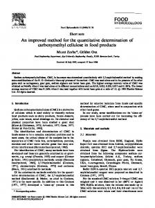
Comparison of the corrected and uncorrected ET measured by the EC method shown in Fig. 1 demonstrates that ET is distinctively underestimated by the EC method. This correction is essential because the energy balance is a prerequisite to be consistent with that of EBBR method. This study uses coincident satellite data, such as Moderate Resolution Imaging Spectroradiometer (MODIS) land surface products related to ET, including Ts and vegetation indices. This data is available at the Earth Observation System (EOS) Gateway Web site (http://redhook.gsfc.nasa.gov/⬃imswww/pub/

AUGUST 2008

715

WANG AND LIANG

under cloudy conditions. To keep the scale consistent and measurements of Ts continuous, the Ts used in this study is calculated from upwelling longwave radiation (Lu) and downwelling longwave radiation (Ld) using the Stefan–Boltzmann law: Ts ⫽ 兵关Lu ⫺ 共1 ⫺ ␧兲Ld兴 Ⲑ共␴␧兲其1Ⲑ4,

共10兲

where ␴ is the Stefan–Boltzmann’s constant (5.67 ⫻ 10⫺8 W m⫺2 K⫺4) and ␧ is the surface broadband emissivity, which we obtained from MODIS narrowband emissivities in the thermal infrared region from the MODIS day–night Ts products (Wang et al. 2005b; Jin and Liang 2006).

3. Outline of the earlier ET algorithm FIG. 1. Comparison of the original (uncorrected) ET measured by the eddy covariance method and ET corrected for the energy imbalance issue [refer to Eq. (7)] at the Goodwin Creek (GC) site from 2002 to 2007.

imswelcome/plain.html). Two global vegetation index products are available from MODIS: the NDVI and the enhanced vegetation index (EVI; Huete et al. 2002). The equations for the indices are NDVI ⫽ 共␳nir ⫺ ␳red兲Ⲑ共␳nir ⫹ ␳red兲

共8兲

and EVI ⫽ 2.5 ⫻ 共␳nir ⫺ ␳red兲Ⲑ共␳nir ⫹ 6 ⫻ ␳red ⫺ 7.5 ⫻ ␳blue ⫹ 1.0兲,

共9兲

where ␳ is reflectance after atmospheric correction, the subscript nir represents the MODIS near infrared band (at 0.841–0.876 ␮m), red represents the MODIS red band (at 0.620–0.670 ␮m), and blue represents the MODIS blue band (at 459–479 ␮m). A 16-day compositing procedure was developed to provide high-quality vegetation index data every 16 days (Van Leeuwen et al. 1999). Two algorithms are used to retrieve Ts from the MODIS thermal (8.4–8.7, 10.78–11.28, and 11.77–12.27 ␮m) and middle infrared (3.66–3.84, 3.929–3.989, and 4.02–4.08 ␮m) spectral regions: the generalized splitwindow algorithm (Wan and Dozier 1996) and the MODIS day–night Ts algorithm (Wan and Li 1997). Field validation indicates that the MODIS Ts at 1-km resolution produced by the split-window algorithm has an accuracy of 1 K (Wan et al. 2002, 2004; Coll et al. 2005; Wang et al. 2005a, 2007a). The Ts at 1-km resolution has a spatial scale much larger than that of the ground measurements. Here, Ts is influenced by solar radiation and vegetation shadow, which result in its large heterogeneity, and MODIS Ts is not available

Wang et al. (2007b) analyzed ground-based and satellite measurements collected at eight EF sites located throughout the SGP from January 2002 to May 2005 and found that the dominant factors driving the seasonal variation of ET are Rn, temperature, and the vegetation index. The strongest correlation is between Rn and ET, and ET increases near linearly with Rn. The Rn-normalized ET increases near linearly with vegetation indices and temperatures. Therefore, we propose a simple regression equation: ET ⫽ Rn共a0 ⫹ a1VI ⫹ a2T 兲,

共11兲

where VI is either EVI or NDVI, and T is either daytime-averaged (or daytime maximum) Ta or Ts. The data collected at the eight SGP sites are used to derive the three parameters a0, a1, and a2 in Eq. (11). ET, predicted with Eq. (11) using a combination of Rn, daytime-averaged Ta and EVI, has an average RMSE of 29.2 W m⫺2. The correlation coefficients between measured and predicted ET vary from 0.88 to 0.96 for the SGP sites. We validated our method using data measured by the EC method at six AmeriFlux sites throughout the United States from 2001 to 2006. The correlation coefficient between predicted and measured ET varies from 0.84 to 0.95, the bias varies from 3.4 to 15.0 W m⫺2, and RMSE varies from 27.4 to 38.7 W m⫺2.

4. Algorithm improvement SM has potentially substantial effects on ET (Gu et al. 2006). According to the two-stage theory of ET, atmospheric demand and available energy determine ET when water supply is sufficient, while soil moisture becomes an important factor controlling ET after soil water supply is deficient (Salvucci 1997). The exponential relationship between SM and ET is derived for unsaturated soil (Komatsu 2003) and veg-

716


VOLUME 9

etation surfaces where the water supply is limited (Davies and Allen 1973): ET ⫽ ␣共Rn ⫺ G兲

冉冊

⌬ 关1 ⫺ exp共⫺␪Ⲑ␪c兲兴, ⌬⫹␥

共12兲

where ␣ ⫽ 1.26 is the Priestley–Taylor parameter, ⌬ ⫽ de*/dT is the gradient of the saturated vapor pressure to the Ta, ␥ ⫽ Cp /␭ is the psychrometric constant, ␪ is the surface SM, and ␪c is a parameter that depends on soil type and wind speed. Detto et al. (2006) found that ET ⫺ ␪ varied with vegetative cover type. Unfortunately, there is no reliable global or regional SM dataset at the spatial scale of kilometers and the temporal resolution of days. For example, Dirmeyer et al. (2004) compared and validated eight available global SM products and found that SM climatologies vary greatly among the products. Schaake et al. (2004) compared the SM fields simulated by four land surface models in North American Land Data Assimilation System (NLDAS) driven by the same meteorological forcing data and initiated at the same time with the same relative SM. Significant differences are found between NLDAS-simulated SM fields and the different models. Therefore, it is essential to use easily obtainable and reliable data to incorporate the influence of SM on ET for an operational algorithm using satellite remote sensing data. Schmugge (1978) argues that there is a strong correlation between observed diurnal land surface temperature range (DTsR) and moisture in the top 5 cm of the soil column (correlation coefficients up to 0.9). Here, DTsR is directly related to ET because as energy consumption by ET increases, the amount of energy heating the earth’s surface decreases, and in turn the DTsR decreases (Wang et al. 2006). Idso et al. (1975) also argued that DTsR is proportional to nearnoon Ts ⫺ Ta over bare soil, and in turn directly related to H and ET. Our study on a semidesert site over the western Tibetan Plateau also shows that the DTsR is proportional to daytime-averaged Ts ⫺ Ta (Wang 2004). Combining Eqs. (1) and (2) in this context produces ET ⫽ Rn ⫺ G ⫺ B共DTsR兲,

共13兲

where B is a parameter that depends on air density and stability conditions. Idso et al. (1975) uses an equation similar to Eq. (13) to estimate ET over bare soil. Global model simulations prove Eq. (13) over vegetationcovered regions (Fig. 13 of Betts 2004). Wang et al. (2006) propose to use DTsR to parameterize evaporative fraction based on the spatial variation of ⌬Ts ⫺ NDVI. Figure 2 illustrates that ET decreases and DTsR increases during the period that the soil dehydrates.

FIG. 2. An example of the time series of the ET, surface soil moisture (2.5-cm depth), and DTsR at the enhanced facility site Elk Falls (EF07) on the U.S. SGP 2002–05.

Based on these studies, we propose to revise Eq. (11) as follows: ET ⫽ Rn共a0 ⫹ a1VI ⫹ a2T ⫹ a3DTsR兲,

共14兲

where VI is EVI or NDVI, T is daytime-averaged (or daytime maximum) Ta or Ts, and DTsR is obtained directly from geostationary and polar-orbit satellite observations [such as those collected by the Advanced Very High Resolution Radiometer (AVHRR) and MODIS (Jin and Dickinson 1999; Jin 2000; Göttsche and Olesen 2001; Aires et al. 2004)]. To estimate the parameters in Eq. (14) accurately, we determined DTsR from ground-based measurements of surface upwelling longwave radiation [see Eq. (10)]. The DTsR parameterizes ET better than SM because ET only depends on soil moisture at root zone depth, and different vegetation physiognomies have access to soil moisture from different layers while the relationship between DTsR and ET is more direct (Idso et al. 1975; Betts 2004; Wang et al. 2006). Incorporating DTsR, besides temperature, into the algorithm to estimate ET under insufficient-water conditions solves a problem encountered in Wang et al. (2007b). Wang et al. (2006) show that ⌬/(⌬ ⫹ ␥) in the Priestley and Taylor (1972) equation, which has the form ⌬ ET ⫽␣ , Rn ⫺ G ⌬⫹␥

共15兲

where ⌬/(⌬ ⫹ ␥) can be calculated directly from temperature, and that ⌬/(⌬ ⫹ ␥) increases linearly with temperature for water-sufficient conditions. However,

AUGUST 2008

WANG AND LIANG

717

TABLE 2. A summary of the regression coefficients in Eq. (14) for different combinations of temperature, vegetation index, and DTsR. We used data collected from 2001 to 2006 at six sites (EF08, EF12, EF15, EF19, EF20, and RA) to derive the parameters (see Table 1 for site information). The vegetation indices EVI and NDVI are obtained from MODIS global 16-day vegetation indices products. We obtained daytime-averaged air temperature (Ta, d), daily maximum air temperature (Ta,m), daytimeaveraged land surface temperature (Ts, d), daily maximum land surface temperature (Ts,m), and diurnal land surface temperature range (TDsR) from ground-based measurements. Surface net radiation is measured by the SIRS system. Combination

a0

a1

a2

a3

EVI, Ta,d, TDsR EVI, Ta,m, TDsR EVI, Ts,d, TDsR EVI, Ts,m, TDsR NDVI, Ta,d, TDsR NDVI, Ta,m, TDsR NDVI, Ts,d, TDsR NDVI, Ts,m, TDsR

0.3541 0.3315 0.3637 0.3383 0.3067 0.2749 0.2925 0.2816

0.6257 0.6437 0.6634 0.6698 0.4425 0.4668 0.4919 0.4834

0.0073 0.0073 0.0062 0.0067 0.0086 0.0085 0.0075 0.0079

⫺0.0134 ⫺0.0143 ⫺0.0144 ⫺0.0159 ⫺0.0141 ⫺0.0150 ⫺0.0153 ⫺0.0170

when the water supply is deficient, ET decreases with Ts, or Ta increases because less energy is used to evaporate water and more energy is used to heat the earth’s surface. The revised algorithm solves this problem by using either Ta or Ts to represent the effect of temperature on ET for water-sufficient conditions and DTsR for water-deficient conditions.

5. Validity at 12 sites over the United States We used the daily ET data collected from 2001 to 2006 at six sites (EF08, EF12, EF15, EF19, EF20, and RA) to derive the four parameters in Eq. (14). The parameters a0, a1, and a2 are similar to those of our previous study (Wang et al. 2007b; Table 2). Here, a3 is negative and its value is similar for various combinations of vegetation indices and temperatures, demonstrating that DTsR is an important and stabilizing influence on ET. Using Eq. (14) and the parameters shown in Table 2, we calculate daytime-averaged ET for the twelve sites. The 16-day-averaged values are used in Eq. (14) because the vegetation indices datasets are 16-day averages. Figure 3 demonstrates that measured and predicted ET using Eq. (14) for a range of EVI, daily maximum Ts, and DTsR are comparable at the six sites used to obtain the parameters. Measured and predicted ET are also comparable at the six validation sites (Fig. 4). Figure 5 is a comparison of the measured and predicted ET for a combination of EVI, daily maximum Ts, and DTsR at all 12 sites. Figures 3–5 demonstrate that Eq. (14) accurately predicts ET over time and space. The

FIG. 3. Comparison of measured (pluses) and predicted ET (points) using Eq. (14) for a range of conditions reflected in variable surface net radiation, EVI, daily maximum land surface temperatures, and DTsR at the six sites used to obtain the coefficients.

equation also accurately simulates the interannual variation at the Goodwin Creek site. Also, notice that there is no substantial difference between the sites used to obtain the parameters and the validation sites. Table 3 demonstrates that Eq. (14) accurately estimates ET. The average correlation coefficient between

FIG. 4. Comparison of the measured (pluses) and predicted ET (points) using Eq. (14) for a range of conditions reflected in variable surface net radiation, EVI, daily maximum land surface temperatures, and DTsR data at the six validation sites.

718


VOLUME 9

ficients between predicted ET- and EC-method-measured ET at the Morgan Monroe temperate deciduous forest (39.32°N, 86.41°W) and the Willow Creek temperate broadleaf evergreen forest (45.91°N, 90.08°W) sites are 0.96 and 0.94, respectively, and the RMSEs are both less than 33 W m⫺2. However, the bias is larger because the EC method underestimated ET without correcting for its imbalance issue. We use the method of Wang et al. (2007b) to calculate the sensitivities of the revised method to the errors of the input data. Assuming that the measurement (or estimation) errors of temperature, EVI, Rn and DTsR are independent, the sensitivity of ET estimated to Rn, EVI, daytime Ta, and DTaR is FIG. 5. Comparison of predicted ET using Eq. (14) and measured ET for all 12 sites. The 12 sites demonstrate a range of topographic, meteorological, and land cover conditions that are reflected in variable surface net radiation, EVI, daily maximum land surface temperatures, and DTsR.

the measured and predicted 16-day-averaged ET for a combination of Rn, EVI, daily maximum Ts, and DTsR is about 0.92 for all sites. The correlation coefficient ranges from 0.89 to 0.98 for the 12 sites. The bias of the predicted 16-day-averaged ET is ⫺1.9 W m⫺2 and varies from ⫺15.2 to ⫹13.6 W m⫺2 for the 12 sites; the RMSE is about 28.6 W m⫺2 for all sites and ranges from 17.3 to 33.2 W m⫺2 for the 12 sites. EVI appears to more accurately estimate ET than NDVI. The range in the range of bias of ET predicted using EVI is about 10 W m⫺2 less than that of NDVI. The smaller range of bias of EVI-estimated ET is because the influence of soil background on NDVI is greater than that of EVI. A statistical comparison of measured and predicted ET for the original and revised methods indicates that the revised method is more accurate based on the correlation coefficients and RMSE (Table 4). More importantly, the revised algorithm works better for water-deficient conditions. This is reflected in an improvement of the accuracy of predicted ET at two droughtstricken sites (EF08 and EF15). The advantage of the revised method is also shown when used to estimate global ET with the original and revised methods (see section 6). EC-method-measured ET must be corrected, because of the energy imbalance issue, before it is compared with ground-based measurements. We compare predicted ET to measured ET at other sites where there was not enough data to correct the ET measurement by the EC method. For example, the correlation coef-

⌬ET ⌬Rn ⫽ , ET Rn

共16兲

⌬EVIa1 ⌬ET ⫽ , ET a0 ⫹ a1EVI ⫹ a2T ⫹ a3DTR

共17兲

⌬Ta2 ⌬ET ⫽ , ET a0 ⫹ a1EVI ⫹ a2T ⫹ a3DTR

共18兲

⌬DTRa3 ⌬ET ⫽ . ET a0 ⫹ a1EVI ⫹ a2T ⫹ a3DTR

共19兲

Consider a situation in which EVI ⫽ 0.35, Rn ⫽ 350 W m⫺2, Ta ⫽ 25°C, and DTaR ⫽ 20°C. The relative error in ET resulting from an error of 4°C in Ta is 6.0%; the relative error in ET resulting from an error of 0.04 in EVI is 5.1%; the relative error in ET caused by an error of 20 W m⫺2 in Rn is 5.7%; and the relative error in ET caused by an error of 4°C in DTsR is 11.0%. The error resulting from the error of Ts and DTsR may partly cancel each other because a2 and a3 have opposite signs. The sensitivity is much less than that of methods using Ts ⫺ Ta (Timmermans et al. 2007). To investigate how the joint uncertainties of the input data affected ET error, we allowed every input parameter to change in increments of 10% error over an error range of ⫾20%. For example, Rn varies from 280 to 420 W m⫺2 in increments of 35 W m⫺2. We calculated the error on ET for every possible combination of input data error (total in 54 ⫽ 625). The error histogram has a standard deviation of 19.1% and an average of 4% (Fig. 6).

6. Global implementation of the improved method We implemented the revised algorithm globally to further demonstrate its reliability. However, DTsR data are currently not available. Fortunately, DTaR is easily obtainable standard data. Because the land sur-

0.917 ⫺10.5 32.7 0.914 ⫺12.8 33.3 0.914 ⫺9.0 33.0 0.914 ⫺10.6 33.1 0.920 ⫺16.2 30.4 0.918 ⫺20.9 30.6 0.915 ⫺17.5 31.2 0.916 ⫺17.1 31.0

0.898 ⫺6.5 33.3 0.900 ⫺12.6 34.0 0.897 ⫺15.5 35.3 0.900 ⫺15.2 33.2 0.894 0.6 32.3 0.893 ⫺7.2 32.7 0.890 ⫺9.8 33.5 0.893 ⫺9.8 32.3

NDVI, Ts,m, TDsR

NDVI, Ts,d, TDsR

NDVI, Ta,m, TDsR

NDVI, Ta,d, TDsR

EVI, Ts,m, TDsR

EVI, Ts,d, TDsR

EVI, Ta,m, TDsR

BI

BH

Item

R Bias RMSE R Bias RMSE R Bias RMSE R Bias RMSE R Bias RMSE R Bias RMSE R Bias RMSE R Bias RMSE

Combination

EVI, Ta,d, TDsR 0.898 ⫺13.2 33.0 0.900 ⫺11.9 32.8 0.904 ⫺11.7 31.7 0.901 ⫺13.1 32.6 0.890 ⫺11.4 35.0 0.892 ⫺12.3 34.3 0.895 ⫺11.7 33.8 0.893 ⫺11.3 34.6

EF07 0.915 ⫺4.5 21.8 0.911 ⫺3.4 22.2 0.915 ⫺0.3 21.8 0.914 ⫺1.6 22.2 0.915 ⫺10.3 21.6 0.911 ⫺11.1 22.0 0.917 ⫺9.1 21.3 0.916 ⫺7.6 21.6

EF08 0.973 1.7 16.7 0.972 2.7 17.2 0.969 5.4 17.9 0.971 4.0 17.3 0.975 1.0 16.4 0.973 ⫺0.4 17.3 0.971 ⫺2.8 17.6 0.973 3.5 16.9

EF09 0.978 2.6 17.5 0.978 3.8 17.7 0.976 4.1 18.3 0.975 2.2 18.7 0.979 4.2 17.5 0.979 3.0 17.2 0.977 3.6 18.2 0.977 3.6 18.7

EF12 0.955 2.7 21.3 0.954 ⫺1.9 21.6 0.946 1.8 23.2 0.951 ⫺0.4 22.1 0.955 ⫺4.9 21.3 0.954 ⫺6.2 21.7 0.946 ⫺2.6 23.1 0.951 ⫺2.6 22.1

EF15 0.938 ⫺6.1 27.2 0.937 ⫺5.5 27.7 0.939 ⫺5.4 26.9 0.937 ⫺6.7 27.5 0.943 ⫺4.5 26.8 0.942 ⫺6.2 26.5 0.943 ⫺5.8 26.6 0.942 ⫺5.1 27.1

EF18 0.909 1.3 33.5 0.906 2.6 34.3 0.912 5.1 32.9 0.910 2.5 33.4 0.906 2.2 34.5 0.902 1.2 34.8 0.909 4.3 33.9 0.908 3.7 34.4

EF19 0.910 ⫺3.1 27.3 0.910 ⫺1.9 27.4 0.908 ⫺1.5 27.4 0.909 ⫺3.5 27.5 0.898 ⫺3.1 29.0 0.897 ⫺4.0 28.6 0.893 ⫺3.6 29.2 0.896 ⫺3.8 29.2

EF20

0.941 ⫺2.6 25.2 0.940 ⫺5.1 25.4 0.939 ⫺2.6 25.4 0.938 ⫺3.7 25.9 0.940 ⫺4.2 25.4 0.938 ⫺9.9 25.9 0.938 ⫺6.1 26.0 0.937 ⫺5.6 26.1

GC

0.906 14.7 32.0 0.906 12.7 32.0 0.901 15.6 32.8 0.899 13.6 33.1 0.891 21.3 34.1 0.891 16.6 34.4 0.884 21.3 35.3 0.880 20.7 35.7

RA

0.922 ⫺2.2 28.2 0.920 ⫺2.3 28.5 0.920 0.0 28.4 0.920 ⫺1.9 28.6 0.916 ⫺2.4 29.3 0.914 ⫺4.9 29.3 0.913 ⫺2.3 29.6 0.914 ⫺2.2 29.6

all

TABLE 3. The statistical parameters (correlation coefficient R bias, and RMSE) for the comparison between 16-day-averaged measured and predicted ET. We used data collected from 2001 to 2006 at six sites (EF08, EF12, EF15, EF19, EF20, and RA) to derive the coefficients in Table 2 by regression. Equation (14) was then used to predict ET with the coefficients in Table 2. ET is measured by the EBBR method at the EF sites over the SGP. ET measured by the EC method at BH, BI, GC, and RA is corrected by the method proposed by Twine et al. (2000). The data are averaged into 16-day periods before the comparison. Bias and RMSE are reported in W m⫺2.

AUGUST 2008 WANG AND LIANG

719

R Bias RMSE R Bias RMSE R Bias RMSE R Bias RMSE R Bias RMSE R Bias RMSE R Bias RMSE R Bias RMSE

Rn, EVI, Ta,d

Rn, NDVI, Ts,m

Rn, NDVI, Ts,d

Rn, NDVI, Ta,m

Rn, NDVI, Ta,d

Rn, EVI, Ts,m

Rn, EVI, Ts,d

Rn, EVI, Ta,m

Item

Combination

0.886 3.0 35.8 0.886 0.7 35.9 0.884 ⫺1.6 36.3 0.885 ⫺0.4 35.3 0.883 21.0 33.8 0.881 17.9 34.0 0.880 15.6 34.2 0.880 16.2 34.0

BH 0.887 ⫺14.3 37.3 0.884 ⫺16.0 37.6 0.883 ⫺15.8 37.6 0.881 ⫺15.2 37.8 0.889 ⫺17.0 35.3 0.886 ⫺20.8 36.0 0.883 ⫺20.6 36.4 0.879 ⫺20.7 36.9

BI 0.882 ⫺16.1 33.1 0.882 ⫺15.2 33.3 0.881 ⫺15.9 33.3 0.878 ⫺15.4 33.9 0.876 ⫺11.1 33.5 0.875 ⫺12.4 33.6 0.874 ⫺13.0 33.7 0.872 ⫺13.3 34.0

EF07 0.881 4.5 25.6 0.876 5.9 26.6 0.873 6.7 27.1 0.869 8.9 28.1 0.882 5.4 25.2 0.878 2.8 25.7 0.875 3.7 26.1 0.871 4.5 26.6

EF08 0.951 ⫺0.7 24.0 0.949 ⫺0.2 23.9 0.947 0.0 24.2 0.947 1.3 24.1 0.948 1.3 25.8 0.946 ⫺0.5 26.1 0.944 ⫺0.3 26.1 0.944 0 26.0

EF09 0.966 1.1 21.5 0.966 1.7 21.6 0.964 0.6 22.2 0.963 1.4 22.6 0.962 5.5 23.7 0.963 4.0 23.3 0.961 2.8 23.8 0.960 2.8 24.1

EF12 0.907 2.5 29.8 0.904 2.4 30.6 0.899 3.9 31.6 0.900 5.0 31.6 0.903 4.1 30.7 0.900 1.8 31.1 0.895 3.2 32.0 0.895 3.1 31.9

EF15 0.943 ⫺5.0 25.8 0.942 ⫺5.0 25.0 0.943 ⫺5.9 24.8 0.943 ⫺4.5 25.2 0.954 ⫺1.7 20.7 0.952 ⫺3.3 21.2 0.953 ⫺4.2 21.0 0.953 ⫺3.7 21.2

EF18 0.896 4.2 34.2 0.895 4.6 34.2 0.893 5.0 34.5 0.891 5.7 35.1 0.893 7.9 33.2 0.893 6.6 33.4 0.890 6.9 33.9 0.888 6.7 34.2

EF19 0.883 ⫺5.9 30.5 0.882 ⫺5.7 30.0 0.878 ⫺6.6 30.5 0.876 ⫺6.0 30.9 0.861 ⫺3.5 31.4 0.860 ⫺5.2 31.5 0.855 ⫺6.1 32.3 0.854 ⫺6.4 32.3

EF20

0.912 3.4 29.3 0.914 0.9 30.3 0.905 0.8 31.8 0.905 2.1 31.9 0.898 ⫺0.1 33.5 0.902 ⫺2.6 33.0 0.892 ⫺2.6 34.4 0.892 ⫺2.0 34.2

GC

0.853 14.1 38.7 0.851 11.8 39.3 0.847 11.3 39.8 0.840 11.6 40.6 0.819 20.2 43.0 0.815 18.5 43.5 0.809 18.0 44.0 0.803 18.3 44.5

RA

all 0.897 ⫺1.4 31.9 0.895 ⫺1.7 32.2 0.892 ⫺1.8 32.7 0.891 ⫺0.8 33.1 0.886 0.9 33.1 0.884 ⫺1.1 33.3 0.881 ⫺1.3 33.8 0.879 ⫺1.1 34.1

TABLE 4. Statistical parameters, variables, and site abbreviations are the same as in Table 3, except that evapotranspiration is predicted using Eq. (11), which does not incorporate DTsR.

720 JOURNAL OF HYDROMETEOROLOGY VOLUME 9

AUGUST 2008

WANG AND LIANG

721

FIG. 6. Histogram of the relative error in ET, calculated when the amount of error on net radiation (Rn), daytime air temperature (Ta), diurnal air temperature range (DTaR), and EVI are all varied over a range of ⫾20% error in increments of 10% error.

FIG. 7. Comparison of ET predicted by Eq. (20) and measured ET for all 12 sites. The 12 sites demonstrate a range of topographic, meteorological, and land cover conditions that are reflected in variable surface net radiation, EVI, daily maximum land surface temperatures, DTsR, and soil moisture.

face typically warms the air during the day for most earth surfaces, DTaR is representative of DTsR, and DTaR is also closely related to ET. Therefore, we replaced DTsR with DTaR in Eq. (14) to yield Eq. (20), based on the data provided in section 2:

tion budget (SRB). The SRB parameters are derived using radiative transfer–based algorithms applied to the cloud data provided by the International Satellite Cloud Climatology Project (ISCCP; Rossow et al. 1996; Rossow and Schiffer 1999). The Initiative II SRB data differ from a similar set of radiative flux parameters derived from ISCCP, called ISCCP-FD (Zhang et al. 2004). Daytime-averaged Ta is calculated from the Climatic Research Unit (CRU), version 5 (New et al. 1999, 2000), 3-hourly meteorological reanalysis data. The DTaR is also from the CRU, version 5, reanalysis dataset. The NDVI is from the Global Inventory Modeling and Mapping Studies (GIMMS) group at the National Aeronautics and Space Administration (NASA) Goddard Space Flight Center (Tucker et al. 2005), which is obtained from National Oceanic and Atmospheric Administration (NOAA)/AVHRR observations. All of the above datasets are monthly averaged and at a spatial resolution of 1° ⫻ 1°. We used Eq. (20) to predict monthly global ET with the described datasets, which are available globally, except for Greenland Island. The ET over the desert is set to zero. We used the University of Maryland, College Park (UMD; Hansen et al. 2000) and MODIS (Friedl et al. 2002) land cover datasets at a spatial resolution of 1° ⫻ 1° to detect desert regions. We compare ET predicted by Eq. (20) to the 15model-simulation-averaged ET from the Global Soil Wetness Project-2 (GSWP-2; Dirmeyer et al. 2006). A total of 15 different state-of-the-art land surface models participated in the project (Dirmeyer et al. 2006). The models are also forced by ISLSCP Initiative II datasets.

ET ⫽ Rn共0.1440 ⫹ 0.6495NDVI ⫹ 0.0090Ta,d ⫺ 0.0163DTaR兲,

共20兲

where Ta,d is the daytime-averaged Ta. Figure 7 shows the comparison of ET predicted with Eq. (20) and measured ET for all 12 sites. The overall correlation coefficient of the comparison of measured and predicted ET with Eq. (20) is 0.88, the RMSE is 34.2 W m⫺2, and the bias is 0.5 W m⫺2 (Table 3). The results of our research indicate that Eq. (20) and DTaR accurately predict global ET, although not as accurately as DTsR, as expected. Here, DTsR and ET are directly related, while the relationship between DTaR and ET is indirect (Wang et al. 2006). We selected the International Satellite Land Surface Climatology Project (ISLSCP) Initiative II global interdisciplinary monthly datasets at a spatial resolution of 1° ⫻ 1° for the period 1986–95 to estimate global ET (http://www.daac.ornl.gov; Hall et al. 2006). Fifty-two ISLSCP datasets, consisting of a common series for the 10-yr period from 1986–95, are coregistered to a common grid and gap filled for continuity using uniform procedures. Hall et al. (2006) supplies a detailed description of the datasets. We provide only a summary of the data used in this study. Here, Rn is calculated from a 3-hourly surface radia-

722


VOLUME 9

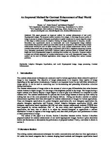
FIG. 8. An example of (top) global ET predicted by Eq. (20) using June 1989 ISCCP Initiative II datasets and (bottom) the corresponding latent heat flux from GSWP-2 datasets. The color bar for both maps is shown at the base of the bottom panel. ET is set at ⫺50 W m⫺2 over the ocean in the figure.

However, their parameterizations of ET, mainly based on the Monin–Obukhov similarity theory, are entirely different from our proposed method (Sellers et al. 1997; Dirmeyer et al. 2006). At the beginning of this paper, we noted that current models cannot accurately simulate ET (Betts and Jakob 2002; Betts et al. 2003; Robock et al. 2003; Mitchell et al. 2004; Yang et al. 2006). Fortunately, studies show that multiple models provide superior results to any individual model (Dirmeyer et al. 2006). ET is equivalent to “latent heat flux” of the GSWP-2 datasets. Although the latent heat flux from GSWP-2 is not accurate enough to be used for reference data, the comparison between measured ET and revised-algorithm-predicted ET will supply useful information when the two independent datasets are in close agreement. Note that daytime-averaged ET is used above, and in the following discussion, whole-day-averaged (daytime and nighttime) ET is compared with the latent heat flux from the GSWP-2 multiple-model simulation. Therefore, the maximum of the ET decreases from about 350

to about 180 W m⫺2. An example of the global ET predicted by Eq. (20) using June 1989 ISCCP Initiative II datasets is compared with the corresponding latent heat flux from GSWP-2 datasets in Fig. 8. Clearly the two datasets have a similar spatial distribution pattern. Their scatterplots are shown in Fig. 9. Predicted and model simulations scatter homogeneously around the 1:1 line, indicating that Eq. (20) can be used on a global scale. In a very few cases, ET predicted by Eq. (20) may be overestimated over arid regions where ET is relatively small, such as over the great deserts of Australia. This results in a small positive bias in the predicted ET because the correspondence of DTaR over arid regions is less than of DTsR. We expect the difference to be reduced when DTsR is used. Figure 10 shows the bias, correlation coefficient, and RMSE of the comparison between the ET predicted by Eq. (20) and the latent heat flux from the GSWP-2 multiple-model average during the 118 months from January 1986 to October 1995. The bias varies from ⫺0.8 to 9.2 W m⫺2, with an average of 4.5 W m⫺2, the

AUGUST 2008

WANG AND LIANG

FIG. 9. An example of the comparison of ET predicted by Eq. (20) using June 1989 ISCCP Initative II datasets and the corresponding latent heat flux from GSWP-2 datasets.

RMSE varies from 16.2 to 22.5 W m⫺2, with an average of 19.8 W m⫺2, and the correlation coefficient varies from 0.71 to 0.91, with an average of 0.82. The 10-yraveraged global ET available is 47.5 W m⫺2. The bias for the Northern Hemisphere winter is relatively large because snow and ice cover the earth’s surface at high latitudes and the proposed method tends to overestimate ET over ice–snow surfaces. The seasonal variation of the bias and RMSE partly reflects the differences in the amount of ratio of land to ocean in the Northern and Southern Hemispheres. We also calculated global ET using the combination of Rn, daytime-averaged Ta, and NDVI [Eq. (11)] to demonstrate the improvement of the accuracy of global ET estimates by incorporating DTaR. Without DTaR, the ET tends to be overestimated when ET is relatively low (e.g., semiarid or arid area) and underestimated when ET is relatively high [e.g., dense forest (not shown here)]. This overestimating and underestimating of ET are solved by incorporating DTsR or DTaR, because arid areas have a higher DTR, which results in lower ET using Eq. (20) or (14). We also calculated the bias, correlation coefficient, and RMSE of the comparison between the ET predicted by Eq. (11) and the latent heat flux from the GSWP-2 multiple-model average during the 118 months from January 1986 to October 1995. The bias varies from 3.0 to 10.3 W m⫺2, with an average of 6.2 W m⫺2, the RMSE varies from 17.2 to 24.5 W m⫺2, with an average of 21.3 W m⫺2, and the correlation coefficient varies from 0.58 to 0.89, with an average of 0.78. The correlation coefficient is much less than that predicted by Eq. (20).

723

FIG. 10. Comparison of the bias, correlation coefficient, and RMSE of ET predicted by Eq. (20) and latent heat flux from GSWP-2 multiple-model average during the 118 months from January 1986 to October 1995.

7. Conclusions Satellite remote sensing is a promising technique for estimating global and regional ET. Current methods to estimate ET, using Ts ⫺ Ta, are sensitive to retrieval errors of Ts and the interpolation errors of Ta from the ground-based point measurements. To improve the accuracy of ET prediction, it is necessary to reduce the sensitivity of the methods to input data error. In a previous study, Wang et al. (2007b) proposed estimating ET by combining Rn, the vegetation index, and temperature. However, the influence of SM on ET was not addressed: SM content does influence ET. Unfortunately, studies show that the relationship between ET and SM is very complicated and varies for different land cover types. In addition, there is no reliable global or regional SM dataset at the spatial scale of kilometers and the temporal resolution of days. This paper uses DTsR (or DTaR) as a variable in an improved algorithm that estimates ET with greater accuracy over vegetated surfaces with an insufficient water supply. Incorporating DTsR solves the problem of using daily-averaged or maximum Ta to parameterize ET (Wang et al. 2007b). That is, ET increases with Ta or Ts for water-sufficient conditions. However, when the soil water is deficient, Ta or Ts increases dramatically because less evaporation occurs. Under water-deficient conditions, ET decreases with increasing Ta or Ts. The revised algorithm solves this problem by using daytimeaveraged or daytime-maximum Ta or Ts to represent the influence of temperature on ET when the water supply is sufficient and using DTsR to represent the

724


influence of water-deficient conditions on ET. Global model simulation demonstrates that DTaR and vapor pressure deficit are tightly coupled (Betts 2004). Therefore, incorporating DTsR into the revised method addresses the effect of vapor pressure deficit on ET. We use ET measured by the EBBR method at eight EF sites on the SGP in the United States and ET measured by the EC method at four AmeriFlux sites from 2001 to 2006 to validate the method. This requires that measurements of ET, ground heat flux, and surface upwelling longwave radiation are available. Our method can accurately estimate ET using only satellite data and Eq. (14). The correlation coefficient between the measured and predicted 16-day-averaged ET for a combination of Rn, EVI, daily maximum Ts, and DTsR values is about 0.92 for all sites and years. The correlation coefficients vary from 0.89 to 0.98 for the 12 sites; the bias of the predicted 16-day-averaged ET is ⫺1.9 W m⫺2. The biases for all sites range from ⫺15.2 to ⫹13.6 W m⫺2. The RMSE of the predicted 16-day-averaged ET is about 28.6 W m⫺2 for all sites and varies from 17.3 to 33.2 W m⫺2 across the 12 sites. The correlation coefficient and RMSE are both better than the previous study, especially for sites affected by drought. The sensitivity of the proposed method to input data error is small. We implemented the revised method to estimate global ET. Because DTsR is not available yet, we used easily obtainable DTaR data to estimate global ET instead. The ET estimated from DTaR is less accurate than DTsR-estimated ET. We calculated global 10-yr monthly ET from the ISLSCP Initiative II global interdisciplinary monthly dataset at a spatial resolution of 1° ⫻ 1° and compared it to the averaged latent heat flux from 15 model simulations of GSWP-2. Although the proposed method is derived from site measurements that have a footprint of several kilometers, depending on wind speed, tower height, and heterogeneity of the surface around the sites, it is reasonable to apply it on a 1° ⫻ 1° scale because both are at the canopy scale. The results indicate that the bias varies from ⫺0.8 to 9.2 W m⫺2, with an average of 4.5 W m⫺2; the RMSE varies from 16.2 to 22.5 W m⫺2, with an average of 19.8 W m⫺2; and the correlation coefficient varies from 0.71 to 0.91, with an average of 0.82. For ET without DTaR, the bias varies from 3.0 to 10.3 W m⫺2, with an average of 6.2 W m⫺2; the RMSE varies from 17.2 to 24.5 W m⫺2, with an average of 21.3 W m⫺2; and the correlation coefficient varies from 0.58 to 0.89, with an average of 0.78. Thus, incorporating DTaR greatly improves the accuracy of the global ET estimates. Predicted ET is even more accurate when DTsR and EVI are used.

VOLUME 9

This study demonstrates that vegetation indexes (NDVI and EVI) from satellite sensors of MODIS accurately predict both the seasonal and the annual variation of ET (Wang et al. 2008, manuscript submitted to Climate Dyn.). Vegetation indexes derived from AVHRR, the Visible Infrared Imager/Radiometer Suite (VIIRS), and the Medium Resolution Imaging Spectrometer (MERIS) on the Envisat satellite data are potentially useable as datasets (Brown et al. 2006; Fensholt et al. 2006; Gallo et al. 2005). Acknowledgments. The ground-based measurements were obtained from the AmeriFlux network (http:// public.ornl.gov/ameriflux/data-get.cfm) and the ARM Program of the U.S. Department of Energy (http:// www.archive.arm.gov/). MODIS satellite data were obtained online (http://redhook.gsfc.nasa.gov/⬃imswww/ pub/imswelcome/plain.html). The International Satellite Land Surface Climatology Project Initiative II global interdisciplinary monthly datasets were downloaded from the Internet (http://www.daac.ornl.gov). GSWP-2 datasets were also downloaded from the Internet (http://haneda.tkl.iis.u-tokyo.ac.jp/gswp2/). We would also like to thank Mike Sparrow for his helpful comments on this manuscript. REFERENCES Aires, F., C. Prigent, and W. Rossow, 2004: Temporal interpolation of global surface skin temperature diurnal cycle over land under clear and cloudy conditions. J. Geophys. Res., 109, D04313, doi:10.1029/2003JD003527. Anderson, M. C., J. M. Norman, G. R. Diak, W. P. Kustas, and J. R. Mecikalski, 1997: A two-source time-integrated model for estimating surface fluxes using thermal infrared remote sensing. Remote Sens. Environ., 60, 195–216. Baldocchi, D., and Coauthors, 2001: FLUXNET: A new tool to study the temporal and spatial variability of ecosystem-scale carbon dioxide, water vapor, and energy flux densities. Bull. Amer. Meteor. Soc., 82, 2415–2434. Bastiaanssen, W. G. M., M. Menenti, R. A. Feddes, and A. A. M. Holtslag, 1998: A remote sensing surface energy balance algorithm for land (SEBAL): 1. Formulation. J. Hydrol., 212, 198–212. Betts, A. K., 2004: Understanding hydrometeorology using global models. Bull. Amer. Meteor. Soc., 85, 1673–1688. ——, and C. Jakob, 2002: Evaluation of the diurnal cycle of precipitation, surface thermodynamics, and surface fluxes in the ECMWF model using LBA data. J. Geophys. Res., 107, 8045, doi:10.1029/2001JD000427. ——, J. H. Ball, and P. Viterbo, 2003: Evaluation of the ERA-40 surface water budget and surface temperature for the Mackenzie River basin. J. Hydrometeor., 4, 1194–1211. ——, M. Zhao, P. A. Dirmeyer, and A. C. M. Beljaars, 2006: Comparison of ERA40 and NCEP/DOE near-surface data sets with other ISLSCP-II data sets. J. Geophys. Res., 111, D22S04, doi:10.1029/2006JD007174. Brown, M. E., J. E. Pinzón, K. Didan, J. T. Morisette, and C. J.

AUGUST 2008

WANG AND LIANG

Tucker, 2006: Evaluation of the consistency of long-term NDVI time series derived from AVHRR, SPOT-Vegetation, SeaWiFS, MODIS, and Landsat ETM⫹ sensors. IEEE Trans. Geosci. Remote Sens., 44, 1787–1793. Caselles, V., M. M. Artigao, E. Hurtado, C. Coll, and A. Brasa, 1998: Mapping actual evapotranspiration by combining Landsat TM and NOAA-AVHRR images: Application to the Barrax area, Albacete, Spain. Remote Sens. Environ., 63, 1–10. Cleugh, H. A., R. Leuning, Q. Mu, and S. W. Running, 2007: Regional evaporation estimates from flux tower and MODIS satellite data. Remote Sens. Environ., 106, 285–304. Coll, C., V. Caselles, J. M. Galve, E. Valor, R. Niclos, J. M. Sanchez, and R. Rivas, 2005: Ground measurements for the validation of land surface temperatures derived from AATSR and MODIS data. Remote Sens. Environ., 97, 288– 300. Davies, J. A., and C. D. Allen, 1973: Equilibrium, potential, and actual evaporation from cropped surfaces in southern Ontario. J. Appl. Meteor., 12, 649–657. Detto, M., N. Montaldo, J. D. Albertson, M. Mancini, and G. Katul, 2006: Soil moisture and vegetation controls on evapotranspiration in a heterogeneous Mediterranean ecosystem on Sardinia, Italy. Water Resour. Res., 42, W08419, doi:10.1029/2005WR004693. Dirmeyer, P. A., Z. Guo, and X. Gao, 2004: Comparison, validation, and transferability of eight multiyear global soil wetness products. J. Hydrometeor., 5, 1011–1033. ——, X. Gao, M. Zhao, Z. Guo, T. Oki, and N. Hanasaki, 2006: GSWP-2: Multimodel analysis and implications for our perception of the land surface. Bull. Amer. Meteor. Soc., 87, 1381–1397. Drexler, J., R. Snyder, D. Spano, and K. T. Paw, 2004: A review of models and micrometeorological methods used to estimate wetland evapotranspiration. Hydrol. Process., 18, 2071–2101. Fensholt, R., I. Sandholt, and S. Stisen, 2006: Evaluating MODIS, MERIS, and VEGETATION vegetation indices using in situ measurements in a semiarid environment. IEEE Trans. Geosci. Remote Sens., 44, 1774–1786. Friedl, M. A., 2002: Forward and inverse modeling of land surface energy balance using surface temperature measurements. Remote Sens. Environ., 79, 344–354. ——, and Coauthors, 2002: Global land cover mapping from MODIS: Algorithms and early results. Remote Sens. Environ., 83, 287–302. Gallo, K., L. Ji, B. Reed, J. Eidenshink, and J. Dwyer, 2005: Multi-platform comparisons of MODIS and AVHRR normalized difference vegetation index data. Remote Sens. Environ., 99, 221–231. Gao, Z., 2005: Determination of soil heat flux in a Tibetan Plateau short-grass prairie. Bound.-Layer Meteor., 114, 165–178. Göttsche, F. M., and F. K. Olesen, 2001: Modelling of diurnal cycles of brightness temperature extracted from METEOSAT data. Remote Sens. Environ., 76, 337–348. Goward, S. N., R. H. Waring, D. G. Dye, and J. Yang, 1994: Ecological remote sensing at OTTER: Satellite macroscale observations. Ecol. Appl., 4, 322–343. Gu, L., and Coauthors, 2006: Direct and indirect effects of atmospheric conditions and soil moisture on surface energy partitioning revealed by a prolonged drought at a temperate forest site. J. Geophys. Res., 111, D16102, doi:10.1029/ 2006JD007161. Hall, F. G., and Coauthors, 2006: ISLSCP Initiative II global data

725

sets: Surface boundary conditions and atmospheric forcings for land–atmosphere studies. J. Geophys. Res., 111, D22S01, doi:10.1029/2006JD007366. Hansen, M. C., R. S. DeFries, J. R. G. Townshend, and R. Sohlberg, 2000: Global land cover classification at 1 km spatial resolution using a classification tree approach. Int. J. Remote Sens., 21, 1331–1364. Huete, A., K. Didan, T. Miura, E. P. Rodriguez, X. Gao, and L. G. Ferreira, 2002: Overview of the radiometric and biophysical performance of the MODIS vegetation indices. Remote Sens. Environ., 83, 195–213. Idso, S. B., R. Y. Jackson, and R. J. Reginato, 1975: Estimating evaporation: A technique adaptable to remote sensing. Science, 189, 991–992. Jiang, L., and S. Islam, 2001: Estimation of surface evaporation map over southern Great Plains using remote sensing data. Water Resour. Res., 37, 329–340. Jin, M., 2000: Interpolation of surface radiative temperature measured from polar orbiting satellites to a diurnal cycle. 2. Cloudy-pixel treatment. J. Geophys. Res., 105, 4061–4076. ——, and R. E. Dickinson, 1999: Interpolation of surface radiative temperature measured from polar orbiting satellites to a diurnal cycle. 1. Without clouds. J. Geophys. Res., 104, 2105– 2116. ——, and S. Liang, 2006: An improved land surface emissivity parameter for land surface models using global remote sensing observations. J. Climate, 19, 2867–2881. Kite, G. W., and P. Droogers, 2000: Comparing evapotranspiration estimates from satellites, hydrological models, and field data. J. Hydrol., 229, 3–18. Komatsu, T. S., 2003: Toward a robust phenomenological expression of evaporation efficiency for unsaturated soil surfaces. J. Appl. Meteor., 42, 1330–1334. Krishnan, P., T. A. Black, N. J. Grant, A. G. Barr, E. H. Hogg, R. S. Jassal, and K. Morgenstern, 2006: Impact of changing soil moisture distribution on net ecosystem productivity of a boreal aspen forest during and following drought. Agric. For. Meteor., 139, 208–223. Mitchell, K. E., and Coauthors, 2004: The multi-institution North American Land Data Assimilation System (NLDAS): Utilizing multiple GCIP products and partners in a continental distributed hydrological modeling system. J. Geophys. Res., 109, D07S90, doi:10.1029/2003JD003823. Monin, A. S., and A. M. Obukhov, 1954: Basic laws of turbulent mixing in the atmosphere near the ground. Tr. Geofiz. Inst., Akad. Nauk SSSR, 24, 163–187. New, M., M. Hulme, and P. Jones, 1999: Representing twentiethcentury space–time climate variability. Part I: Development of a 1961–90 mean monthly terrestrial climatology. J. Climate, 12, 829–856. ——, ——, and ——, 2000: Representing twentieth-century space–time climate variability. Part II: Development of 1901– 96 monthly grids of terrestrial surface climate. J. Climate, 13, 2217–2238. Nishida, K., R. R. Nemani, S. W. Running, and J. M. Glassy, 2003: An operational remote sensing algorithm of land surface evaporation. J. Geophys. Res., 108, 4270, doi:10.1029/ 2002JD002062. Norman, J. M., W. P. Kustas, and K. S. Humes, 1995: A twosource approach for estimating soil and vegetation energy fluxes in observations of directional radiometric surface temperature. Agric. For. Meteor., 77, 263–293. ——, ——, J. H. Prueger, and G. R. Diak, 2000: Surface flux es-

726


timation using radiometric temperature: A dual-temperature-difference method to minimize measurement errors. Water Resour. Res., 36, 2263–2274. Oku, Y., and H. Ishikawa, 2004: Estimation of land surface temperature over the Tibetan Plateau using GMS data. J. Appl. Meteor., 43, 548–561. Peres, L. F., and C. C. DaCamara, 2004: Land surface temperature and emissivity estimation based on the two-temperature method: Sensitivity analysis using simulated MSG/SEVIRI data. Remote Sens. Environ., 91, 377–389. Prata, A. J., and R. P. Cechet, 1999: An assessment of the accuracy of land surface temperature determination from the GMS-5 VISSR. Remote Sens. Environ., 67, 1–14. Priestley, C. H. B., and R. J. Taylor, 1972: On the assessment of surface heat flux and evaporation using large-scale parameters. Mon. Wea. Rev., 100, 81–92. Prince, S. D., S. J. Goetz, R. O. Dubayah, K. P. Czajkowski, and M. Thawley, 1998: Inference of surface and air temperature, atmospheric precipitable water and vapor pressure deficit using Advanced Very High Resolution Radiometer satellite observations: Comparison with field observations. J. Hydrol., 212, 230–249. Robock, A., and Coauthors, 2003: Evaluation of the North American Land Data Assimilation System over the southern Great Plains during the warm season. J. Geophys. Res., 108, 8846, doi:10.1029/2002JD003245. Rossow, W. B., and R. A. Schiffer, 1999: Advances in understanding clouds from ISCCP. Bull. Amer. Meteor. Soc., 80, 2261– 2287. ——, A. W. Walker, D. E. Beuschel, and M. D. Roiter, 1996: International Satellite Cloud Climatology Project (ISCCP): Documentation of new cloud data sets. World Meteorological Organization Tech. Rep. WMO/TD-737, 115 pp. Rowntree, P. R., 1991: Atmospheric parameterization for evaporation over land: Basic concept and climate modeling aspects. Land Surface Evaporation Fluxes: Their Measurements and Parameterization, T. J. Schmugge and J. C. André, Eds., Springer-Verlag, 5–30. Salvucci, G. D., 1997: Soil and moisture independent estimation of stage-two evaporation from potential evaporation and albedo or surface temperature. Water Resour. Res., 33, 111–122. Schaake, J. C., and Coauthors, 2004: An intercomparison of soil moisture fields in the North American Land Data Assimilation System (NLDAS). J. Geophys. Res., 109, D01S90, doi:10.1029/2002JD003309. Schmugge, T., 1978: Remote sensing of surface soil moisture. J. Appl. Meteor., 17, 1549–1557. Sellers, P. J., and Coauthors, 1997: Modeling the exchanges of energy, water, and carbon between continents and the atmosphere. Science, 275, 502–509. Sun, D., R. T. Pinker, and J. B. Basara, 2004: Land surface temperature estimation from the next generation of geostationary operational environmental satellites: GOES M–Q. J. Appl. Meteor., 43, 363–372. Timmermans, W. J., W. P. Kustas, M. C. Anderson, and A. N. French, 2007: An intercomparison of the Surface Energy Balance Algorithm for Land (SEBAL) and the Two-Source Energy Balance (TSEB) modeling schemes. Remote Sens. Environ., 108, 369–384. Tucker, C. J., J. E. Pinzon, M. E. Brown, D. A. Slayback, E. W. Pak, R. Mahoney, E. F. Vermote, and N. El Saleous, 2005:

VOLUME 9

An extended AVHRR 8-km NDVI dataset compatible with MODIS and SPOT vegetation NDVI data. Int. J. Remote Sens., 26, 4485–4498. Twine, T., and Coauthors, 2000: Correcting eddy-covariance flux underestimates over a grassland. Agric. For. Meteor., 103, 279–300. Van Leeuwen, W., A. Huete, and T. Laing, 1999: MODIS vegetation index compositing approach: A prototype with AVHRR data. Remote Sens. Environ., 69, 264–280. Venturini, V., G. Bisht, S. Islam, and L. Jiang, 2004: Comparison of EFs estimated from AVHRR and MODIS sensors over South Florida. Remote Sens. Environ., 93, 77–86. Verstraeten, W. W., F. Veroustraete, and J. Feyen, 2005: Estimating evapotranspiration of European forests from NOAA imagery at satellite overpass time: Towards an operational processing chain for integrated optical and thermal sensor data products. Remote Sens. Environ., 96, 256–276. Wan, Z., and J. Dozier, 1996: A generalized split-window algorithm for retrieving land-surface temperature from space. IEEE Trans. Geosci. Remote Sens., 34, 892–905. ——, and Z.-L. Li, 1997: A physics-based algorithm for retrieving land-surface emissivity and temperature from EOS/MODIS data. IEEE Trans. Geosci. Remote Sens., 35, 980–996. ——, Y. Zhang, Q. Zhang, and Z.-L. Li, 2002: Validation of the land surface temperature products retrieved from Terra Moderate Resolution Imaging Spectroradiometer data. Remote Sens. Environ., 83, 163–180. ——, ——, ——, and ——, 2004: Quality assessment and validation of the MODIS global land surface temperature. Int. J. Remote Sens., 25, 261–274. Wang, K., 2004: A study on surface characteristics over the Tibetan Plateau using satellite remote sensed data and groundbased measurements. Ph.D. dissertation, Peking University, 144 pp. ——, J. Liu, Z. Wan, P. Wang, M. Sparrow, and S. Haginoya, 2005a: Preliminary accuracy assessment of MODIS land surface temperature products at a semi-desert site. Optical Technologies for Atmospheric, Ocean, and Environmental Studies, D. Lu and G. Matvienko, Eds., International Society for Optical Engineering (SPIE Proceedings, Vol. 5832), 452–460. ——, Z. Wan, P. Wang, M. Sparrow, J. Liu, X. Zhou, and S. Haginoya, 2005b: Estimation of surface long wave radiation and broadband emissivity using Moderate Resolution Imaging Spectroradiometer (MODIS) land surface temperature/ emissivity products. J. Geophys. Res., 110, D11109, doi:10.1029/2004JD005566. ——, X. Zhou, W. Li, J. Liu, and P. Wang, 2005c: Using satellite remotely sensed data to retrieve sensible and latent heat fluxes: A review (in Chinese with English abstract). Adv. Geosci., 20, 42–48. ——, Z. Li, and M. Cribb, 2006: Estimation of evaporative fraction from a combination of day and night land surface temperature and NDVI: A new method to determine the Priestley–Taylor parameter. Remote Sens. Environ., 102, 293–305. ——, Z. Wan, P. Wang, M. Sparrow, J. Liu, and S. Haginoya, 2007a: Evaluation and improvement of the MODIS land surface temperature/emissivity products using ground-based measurements at a semi-desert site on the western Tibetan Plateau. Int. J. Remote Sens., 28, 2549–2565. ——, P. Wang, Z. Li, M. Cribb, and M. Sparrow, 2007b: A simple method to estimate actual evapotranspiration from a combi-

AUGUST 2008

WANG AND LIANG

nation of net radiation, vegetation index, and temperature. J. Geophys. Res., 112, D15107, doi:10.1029/2006JD008351. Wilson, K., and Coauthors, 2002: Energy balance closure at FLUXNET sites. Agric. For. Meteor., 113, 223–243. Yang, F., H.-L. Pan, S. K. Krueger, S. Moorthi, and S. J. Lord, 2006: Evaluation of the NCEP Global Forecast System at the ARM SGP Site. Mon. Wea. Rev., 134, 3668–3690. Yang, K., T. Koike, H. Ishikawa, and Y. Ma, 2004: Analysis of the

727

surface energy budget at a site of GAME/Tibet using a single-source model. J. Meteor. Soc. Japan, 82, 131–153. Zhang, Y.-C., W. B. Rossow, A. A. Lacis, V. Oinas, and M. I. Mishchenko, 2004: Calculation of radiative fluxes from the surface to top of atmosphere based on ISCCP and other global data sets: Refinements of the radiative transfer model and the input data. J. Geophys. Res., 109, D19105, doi:10.1029/ 2003JD004457.