An Improved Particle Filter for Non-linear Problems - CiteSeerX

An Improved Particle Filter for Non-linear Problems James Carpenter

Peter Clifford y

Paul Fearnhead

y Address for correspondence: Department of Statistics, University of Oxford, 1 South Parks Road, Oxford, OX1 3TG, UK. Abstract The Kalman filter provides an effective solution to the linear-Gaussian filtering problem. However, where there is nonlinearity, either in the model specification or the observation process, other methods are required. We consider methods known generically as particle filters, which include the condensation algorithm and the Bayesian bootstrap or sampling importance resampling (SIR) filter. These filters represent the posterior distribution of the state variables by a system of particles which evolves and adapts recursively as new information becomes available. In practice, large numbers of particles may be required to provide adequate approximations and for certain applications, after a sequence of updates, the particle system will often collapse to a single point. We introduce a method of monitoring the efficiency of these filters, which provides a simple quantitative assessment of sample impoverishment and show how to construct improved particle filters which are both structurally efficient, in terms of preventing the collapse of the particle system and computationally efficient in their implementation. We illustrate with the classic bearings-only tracking problem. Keywords: Kalman filter, Condensation algorithm, Bayesian bootstrap filter, Sampling importance resampling (SIR) filter, Sequential estimation, Markov Chain Monte Carlo (MCMC), Importance resampling.

1 Introduction The Bayesian approach to dynamic state estimation problems involves the construction of the probability density function (PDF) of the current state of an evolving system, given the accumulated observation history. For linear Gaussian models where the PDF can be summarised by means and covariances, the calculation is carried out in terms of the familiar updating equations of the Kalman filter. In general, for nonlinear, non-Gaussian models, there is no simple way to proceed. Two difficulties must be resolved: how to represent a general PDF using finite computer storage and how to perform the integrations involved in updating the PDF when new data are acquired. Several approximate methods have been proposed. These include the extended Kalman filter [1, 2], the Gaussian sum filter [3], approximating the first two moments of the PDF [4,5] and numerical integration over a grid of points in the state space [6–10] . However, none of these methods can be applied automatically. Typically, they have to be tuned to take account of features of each specific problem. For example, in grid-based methods the number and location of the grid points has to be decided upon, usually by a process of trial and error. Furthermore, updating the distribution of the state of the system as new data arrive usually entails a formidable computational overhead.

1

There is now a substantial literature concerned with simulation based filters in which the required PDF is represented by a scatter of particles which propagate through the state space [9,11–19]. The propagation and adaptation rules are chosen so that the combined weight of particles in a particular region will approximate the integral of the PDF over the region. Such filters have been variously described as Bayesian bootstrap, condensation, Monte-Carlo and Metropolis-Hastings importance resampling filters. For the purposes of this paper we adopt the term Monte Carlo particle filter or particle filter for short. Gordon, Salmond and Smith [14] demonstrate the effectiveness of a simple algorithm for particle evolution for various nonlinear filtering applications. Their method has become known as the Sampling Importance Resampling (SIR) filter or, more commonly in the engineering literature, the Bayesian bootstrap filter. The standard SIR filter is vulnerable to sample impoverishment [17, 20–22], so that the particle distribution gives a poor approximation of the required PDF. In extreme cases, after a sequence of updates the particle system can collapse to a single point. In less extreme cases, although several particles may survive, there is so much internal correlation that summary statistics behave as if they are derived from a substantially smaller sample. To compensate, large numbers of particles are required in realistic problems. In this paper we show how sample impoverishment can be quantified. We introduce modifications which we demonstrate to have superior performance to the SIR filter both in terms of combating sample impoverishment and in computational cost. In section 2 we give a brief review of Bayesian filtering theory. In Section 3 we reformulate the SIR filter as an evolving random measure and show that variance reduction techniques from the theory of MonteCarlo integration [23] can be applied. Section 4 introduces the modified particle algorithm, and we note that the computational complexity of each update calculation can be reduced from O (N log N ) to O (N ) where N is the number of particles. Section 5 demonstrates how to quantify sample impoverishment and Section 6 contains an application of the new algorithm to the classic bearings-only tracking problem. Finally Section 7 presents some conclusions.

2 Bayesian Filtering Following Gordon, Salmond and Smith [14] we represent the state vector at time k by xk satisfies

2 Rn , which

xk+1 = fk (xk ; wk )

where fk : R n  Rm ! Rn is the system transition function and wk is a noise term whose known distribution is independent of time. At each discrete time point an observation yk 2 R p is obtained, related to the state vector by

yk = hk (xk ; vk )

where hk : Rn  Rr ! Rp is the measurement function and vk 2 Rr is another noise term whose known distribution is independent of both the system noise and time. We write Dk for (y1 ; :::; yk ), the available information at time k , and assume the PDF of x1 ; the initial state of the system, is known so that p(x1 jD0 ) = p(x1 ). We then wish to obtain the PDFs of p(xk jDk ) : k  2, which are given by the 3 equations:

Z

p(xk jDk?1 ) = p(xk jxk?1 )p(xk?1 jDk?1 ) dxk?1

2

(1)

and

p(xk jDk ) = p(ykpjx(ky)pjD(xk jD)k?1 ) ,

(2)

p(yk jDk?1 ) = p(yk jxk )p(xk jDk?1 ) dxk .

(3)

k

Z

where

k?1

The basic SIR algorithm, which provides approximate solutions to (1–3) is given by Gordon, Salmond and Smith [14]. See also Section 3.1 below.

3 Random measures Particle filters work by providing a Monte Carlo approximation to the PDF which can be easily updated to incorporate new information as it arrives. The Monte Carlo approximation to a PDF p(xk ) at time k consists of a set of random nodes in the state space (sik )i=1:::N , termed the support, and a set of associated weights (mik )i=1:::N summing to 1. The support and the weights together form a random measure. The objective is to choose a measure so that

N X i=1

g(sik )mik 

Z

g(xk )p(xk ) dx

(4)

for typical functions g of the state space. This is an approximation in the sense that the left-hand side of (4) converges (in probability) to the right-hand side as N ! 1 [24].

A simple example of a random measure is obtained by sampling values (sik )i=1:::N independently from p(xk ), and attaching equal weights mik = N ?1 ; i = 1; : : : ;N to the values. The left-hand side of (4) i is then the sample average N i=1 g(sk )=N . Importance sampling [25] generalises this by sampling i (sk )i=1:::N from an importance PDF f (xk ) and attaching importance weights mik = Ap(sik )=f (sik ), i i where A?1 = N i=1 p(sk )=f (sk ).

P

P

More sophisticated Monte Carlo integration techniques [23] are also available. Stratified sampling is of particular relevance. Suppose that a PDF p(x) is made up of contributions from N distinct subpopulations or strata, so that p(x) is a mixture of the form

p(x) =

N X i=1

i pi (x);

P = 1. Sampling theory [26] tells us that a population quantity each pi (x) is a PDF and N i i Rwhere g(x)p(x)dx can be estimated efficiently by sampling a fixed number M from each of the strata, with =1

i

M1 + : : : + MN = N . The greatest efficiency is attained with the Neyman allocation Mi / ii, where i2 is the variance of g(x) in the ith stratum. In practice, either because the variances are unknown or because a number of different functions are to be monitored, the proportional allocation Ni / i is frequently used. Except in certain degenerate cases, this proportional allocation can be shown to be more efficient than simple random sampling from p(x) [26]. 3

A random measure (~ si ; mi )i=1:::N which approximates p(x) can be converted, by resampling, into an equally weighted measure which approximates a simple random sample from p(x). Resampling consi ; mi )i=1:::N , i.e. the discrete distribution with sists of sampling (s1 ; : : : ;sN ) with replacement from (~ i i support points (~ s ) and probabilities (m ). This leads to a new random measure (si ; N ?1 )i=1:::N where now the weights are equal but, typically, there are fewer distinct points in the support. Resampling plays a important role in the SIR filter but we will show that improved approximations are obtained by using the weighted measure before resampling rather than resampling and then using the unweighted measure. Intuitively, this is not surprising because we would expect a set of weighted sample points to carry more information than an equal number of unweighted points.

3.1 The standard SIR algorithm as a random measure The basic SIR algorithm given by Gordon Salmond and Smith [14] is as follows. Initialisation Begin by simulating a sample (si1 )i=1:::N from p(x1 ). In other words, start from a random measure with equal weight on each of the N sample values. Preliminaries (step k) Assume that we have an equally weighted random measure (sik?1 ; N ?1 )i=1:::N , approximating p(xk?1 jDk?1 ). Prediction

Estimate the density p(xk jDk ), up to a normalising constant K , by the mixture

p(xk jDk ) = K

N X i=1

p(xk jsik?1 )p(yk jxk ):

Take exactly one sample point from each of the N strata, by generating support points s~ik from the system model, with importance weights

i mik = PNp(yk js~k ) j ; j =1 p(yk js~k )

(5)

= fk?1 (sik?1 ; wki ?1 ) (6)

sik ; mik )i=1:::N to obtain an equally weighted random Update Resample from the random measure (~ measure (sik ; N ?1 )i=1:::N . In other words, sample N times, independently with replacement, from the set (~ sik )i=1:::N , with probabilities (mik )i=1:::N . A rapid algorithm for the update step, is given in Subsection 4.1.

3.2 Variance reduction at the update stage The analysis in this section provides the motivation for the improved filter discussed below. Suppose that we wish to estimate

Z

k = p(xk jDk )g(xk )dxk ; 4

the mean value of some function g of the state of the system at time k . Using the resampled values from the SIR filter, this can be estimated by

^k = N ?1

N X i=1

g(sik ):

However, an unnecessary element of random noise is introduced by this approach. Suppose sample from p(xk jDk?1 ) then the quantity k can be estimated more precisely by

~k =

N X i=1

mik g(~sik );

(~sik ) is a (7)

where mik is given in (6). To see this, we note that ^k can be written as

^k = N ?1

N X i=1

Zi g(~sik )

where (Z1 ; : : : ; ZN ) is a multinomial distributed vector with probabilities therefore the expected value of ^k .

(mik ). The quantity ~k is

Calculating variances we find that, for N large, Var ^k

 Var ~k + N1 Var g(xk ),

(8)

where the last term is the variance that ~k would have if (sik )i=1:::N was a simple random sample of size N from p(xk jDk ). Details of the derivation are omitted for brevity. It follows that the variance of ~k is always smaller than that of ^k . In fact when the observation yk is not informative, i.e. mik = N ?1 then the variance of ^k is effectively double that of ~k .

4 Efficient Particle Filters As a refinement of the SIR filter it has been suggested [20] that a larger number of values, say 10, should be sampled from each stratum. At the resampling stage, a sample of size N is then selected from the 10  N predicted values, in order to restore the size of the support set to N . It has also been suggested [22] that a simple random sample should be drawn from the mixture distribution (5). However sampling theory indicates that greater accuracy can be achieved by stratified sampling. We can write p(xk jDk ) from (5) in the form

p(xk ) = where

N X i=1

i pi(xk )

R p(x jsi )p(y jx ) dx i = PN R k k? i k k k p(x js )p(y jx ) dx 1

i=1

k k?1 5

k k

k

and

p(x jsi )p(y jx ) pi (xk ) = R p(x kjsi k?)1p(y kjx k) dx : k k?1

k k

k

In this paper we will only consider stratification by the proportional allocation. Ideally we should take Mi = N i but in practice these quantities are unlikely to be exact integers. We can however arrange that Mi are integer variables with small variances and the correct expected value. Our Algorithm 2 in Section 4.1 achieves this while ensuring that jMi ? N i j is always less than 1. Another simple suggestion [27] is to take Mi to be the integer part of N i , and then to add 1 randomly with probability equal to the fractional part of N i . A disadvantage of this method is that the population of particles will fluctuate in size (although it will never die out completely). In practice, the quantities i and pi (xk ) may be difficult to deal with and importance sampling is necessary. Combining the preceding steps the proposed particle filter is as follows: Initialisation Start from a random measure with sampling, which approximates the PDF p(x1 ).

N

support points, possibly obtained by stratified

Preliminaries (step k) Assume that we have a random measure p(xk?1 jDk?1 ). Prediction

(sik?1 ; mik?1 )i=1:::N , approximating

Estimate the density p(xk jDk ), up to a normalising constant K , by

p(xk jDk ) = K

N X i=1

mik?1 p(xk jsik?1 )p(yk jxk ):

Construct an importance PDF

p^(xk ) =

(9)

N X ^ i=1

i p^i(xk )

Take a stratified sample from this density using Algorithm 2, with Mi sample points in the ith category, where Mi has expected value N ^i . Update

For each i, sample Mi support points (sjk ) from pi (xk ), with importance weights given by

mjk /

mik?1 p(sjk jsik?1 )p(yk jsjk ) ^i p^i(sjk )

The updated random measure is then given by 1.

i? X 1

for

`=1

M` < j 

Xi `=1

M` :

(sjk ; mjk )j =1:::N , where the weights are scaled to sum to

Properties of the updated state distribution can be estimated using the random measure as in (7). If an approximate sample from the state distribution is required it can be obtained by simple random sampling from the random measure as described in Section 3. Note that once the stratification numbers 6

have been calculated, there is only one sampling operation at each update. Carrying forward the weights (mk?1 ) at the update step, eliminates the resampling phase of the standard SIR filter. Construction of the importance PDF is necessarily problem specific. We work through an example in Section 6.

4.1 Reducing the computational complexity of particle filters Sampling of N values from a discrete distribution (si ; mi )i=1:::N , can be carried out by simulating standard uniform variables (ui )i=1:::N and then using binary search to find the value j , and hence xj , corresponding to

P where Qj = j` m` and Q =0

Qj?1 < ui  Qj ;

0

= 0.

Binary search is commonly used to implement the updating stage of the SIR algorithm. However it is not efficient. To obtain a sample of size N , by this means, takes O (N log N ) calculations; the log(N ) term arises from the binary search. A more efficient method is to simulate N + 1 exponentially distributed variables t0 ; : : : ;tN , using ti = ? log(ui ), calculate the running totals Tj = j`=0 t` , and then merge (Tj ) and (Qj ). The algorithm is based on the well known method of simulating order statistics [28].

P

O(N ) algorithm for the SIR filter i = 0; j = 1 do while i < N if Qj TN > Ti then i = i + 1; output sj

Algorithm 1

else

j =j +1

end if end do

For precise proportional stratification, the objective is to ensure that the number of points in the ith category is as close as possible to N i . Label the categories si = i. The output will consist of N category labels, with the property that the expected number of labels of category i will be equal to N i and the actual number will differ from the expected number by no more than 1.

O(N ) algorithm for stratification T = unif(0; 1)=N ; j = 1; Q = 0; i = 0 do while T < 1 if Q > T then T = T + 1=N ; output si

Algorithm 2

else pick k in fj; : : : ; N g

i = sk Q = Q + i switch (sk ; k ) j =j +1

with

(sj ; j ) 7

end if end do

5 A diagnostic for sample impoverishment All the particle filters we compare in Section 6 are capable of approximating the posterior distributions of the state variables in a statistical sense. They differ in terms of the accuracy with which properties of the state distribution can be estimated. For the purposes of comparison, the effective sample size is an obvious quantity to compute. This is the sample size that would be required for a simple random sample from the target PDF to achieve the same estimating precision as the particle filter. Since some properties of the state distribution may be estimated well, and some poorly, the effective sample size will depend on what is being estimated. Suppose that the property to be estimated is

Z

k = g(xk )p(xk jDk )dxk ; and let

zk =

N X i=1

mik g(~sik ), vk =

N X i=1

mik g2 (~sik ) ? zk2

be the filter estimates of  and  2 , the variance of g (xk ) given Dk as in Equation (8). Note that, if  is estimated by using the average value of g (xk ) in a simple random sample of size N  from p(xk jDk ), the estimate will have a variance of  2 =N  . To evaluate the effective sample size, we use a technique borrowed from classical ‘analysis of variance’ in statistics. 1. Run the filter independently particles.

M

times, obtaining

2. For each replicate, at step k , calculate zkj and vkj ; j

M

independent replicates, each based on

N

= 1; : : : ;M .

3. Calculate zk and vk , the average values over the M replicates.

4. The effective sample size is then M vk =

PM (zj ? z ) . k j k 2

=1

To see this, we equate two estimates of the variance of zk : one based on the variance between replicates and the other based on the notional variance that an estimate would have if it was a sample average of a simple random sample of size N  , i.e.

X M ?1 (z j ? zk )2 = M

j =1

k

2  vk : N N

The effective sample size is then obtained by solving for N  . We advocate the use of this diagnostic generally, in assessing the performance of Monte Carlo filters. The smaller the effective sample size is, the less reliable the filter is. In principle, a Bayesian filter 8

should be assessed by looking at its performance averaged over the population of trajectories generated by the system model. However, for non-linear problems it may happen that most of the trajectories are simple to filter and only a few are ‘difficult cases’. It is therefore helpful to see how the filter performs for typical examples of these difficult cases. An example of such a problem is given in Section 6. The integrated correlation time in Markov chain Monte Carlo (MCMC) calculations in non-dynamic problems [29] and the effective sample size play similar roles. Neither of these diagnostics checks to see whether there is convergence to the right distribution. A noisy biased filter may have a large effective sample size but the sample will not have come from the correct distribution. To check for bias, the proposed particle filter will need to be compared with filters which are known to perform correctly.

6 Bearings-only tracking In this example an object moves in the (;  ) plane according to a second order model

xk = xk?1 + ?wk , where xk

= (; ; _ ; _ )Tk ; wk = (w ; w )Tk ,

0 =B @

1 0 0 0

1 1 0 0

0 0 1 0

0 0 1 1

1 C A

and

0 ?=B @

(10)

1 1 0 0

0 0 1 1

1 C A:

(11)

The system fluctuations wk = (w ; w )Tk are independent zero-mean Gaussian white noise. The model essentially assumes that the velocity evolves like Brownian motion. The ‘leap-frog’ discretisation is slightly non-standard. The state variables _ k and _ k are the velocities at time k ? 1=2. Positions are updated by using a midpoint approximation to the integrated velocities. Velocities at step k would be approximated by (_ k + _ k+1 )=2 and (_ k + _ k+1 )=2. There is an equivalent formulation of the leap-frog algorithm in which (_ k ; _ k ) are the velocities at time k + 1=2 [22, 30]. The matrix ? is then modified in the obvious way. We will use parameters which are compatible with an example considered by Gordon, Salmond and Smith [14] who use a different integration scheme. The observations are a sequence of bearings:

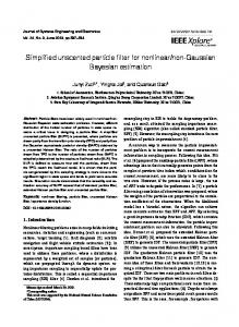
yk = tan?1 (k =k ) + vk The initial state of the object is x1 = (?0:05; 0:001; 0:7; ?0:055)T . The system noise variables w ; w have variance  2 = 0:0012 and the observation error vk has variance  2 = 0:0052 . We consider an observed trajectory which passes close by the observer who is fixed at the origin. See Figure 1. We adopt the same prior distribution of the starting configuration as Gordon, Salmond and Smith [14]. To construct the importance PDF we consider the ith component of (9)

Kmik?1 p(xjs)p(yjx)

(12)

where we have replaced sik?1 by s, yk by y and xk by x for notational convenience. Conditional on s the density of x depends only on (;  ). Converting (;  ) and (E( js); E( js)) to polar coordinates as 9

(r; ) and (; ), respectively, it follows that (12) is proportional to

mik?1re?(r2 +2 ?2r cos(?))=(2 2 )?(y?)2 =(22 ) 2 2 2 2 2 2 2 = mik?1re?(r? cos(?)) =(2 )? sin (?)=(2 )?(y?) =(2 ) : Our importance PDF is obtained by replacing sin( ? ) by  ? , giving the PDF ^i f ()f (rj) where

f (rj) / re?(r? cos(?))2 =(2 2 ) and f ( ) is the Gaussian PDF with mean ( 2 2 + y 2 )=(2  2 +  2 ) and variance  2  2 =(2  2 +  2 ) P ^ = 1. Both f () and f (rj) can and the normalising constants have been absorbed into ^i with N i=1 i be sampled directly using standard methods.

All the filters were initialised by taking samples of size N = 5000 from p(x2 jD2 ), obtained using the Metropolis Hastings Algorithm as described in [30]. The distribution of these samples was checked against a numerical evaluation of p(x2 jD2 ) and found to agree closely. The samples were also checked for independence by computing auto-correlations during the Metropolis Hastings simulations. The effective sample sizes were calculated using M = 1000 replicates. Each of the different filtering methods were successively initialised from each of the M starting configurations The results, for various methods, are presented in Table 1. We calculate effective sample sizes for the filter estimates of the mean range and the mean bearing at each step. In all cases, there is greater sample impoverishment for the range calculations than for the bearings. The ‘Improved Reweighted’ filter is an implementation of the particle filter described in the paper, with precisely stratified sampling as in Algorithm 2. The ‘Multinomial Reweighted’ filter carries weights forward as in the improved filter, but samples the strata multinomially using Algorithm 1 (with mi = i ). The ‘Two Stage’ algorithm [22] samples strata multinomially, but resamples after each step, to obtain equally weighted particles. The ‘Standard SIR’ [14] is included for comparison. Note that our implementation of the basic SIR algorithm (Subsection 3.1 ) does not incorporate the ad hoc modifications of added jitter and prior editing suggested by Gordon, Salmond and Smith [14].

7 Conclusions We have shown how to reduce the computational cost of implementing particle filters. We have proposed an improved particle filter and demonstrated its superior performance. While the filter is more complicated to implement and, unlike the standard SIR filter, needs to be tailored to the problem in hand, the computational gains are substantial. Further, we have introduced a diagnostic for sampling inefficiency which allows us to compare the performance of various Monte Carlo filters. We advocate the use of this diagnostic as a general tool in the analysis of sequential Monte Carlo algorithms. All of the filters we have discussed suffer from substantial sample impoverishment. In principle this could be monitored using our diagnostic and compensated for dynamically, by adjusting the number of particles at critical stages. We believe that there is scope for even greater variance reduction by the use of more efficient Monte Carlo integration techniques. 10

8 Acknowledgements This research was supported by DERA grant WSS/U1172. Paul Fearnhead has an EPSRC studentship. We are grateful to Neil Gordon and David Salmond for a number of stimulating conversations.

References [1] JAZWINSKI, A. H. ‘Stochastic processes and filtering theory’, Academic Press, 1973. [2] M OON , J. R. AND S TEVENS , C. F. ‘An approximate linearisation approach to bearings-only tracking’, IEE Target tracking and data fusion: Colloquium digest 96/253, 1996, pages 8/1–8/14. [3] A LSPACH , D. L. AND S ORENSON , H. W. ‘Non-linear Bayesian estimation using Gaussian sum approximation’, IEEE Trans. Auto. Control, 1972, 17, pp. 439–447. [4] M ASRELIEZ, C. J. ‘Approximate non-Gaussian filtering with linear state and observation relations’, IEEE Trans. Auto. Control, 1975, 20, pp. 107–110. [5] W EST, M., H ARRISON , P. J., AND M IGON , H. S. ‘Dynamic generalised linear models and Bayesian forecasting (with discussion)’, J. Am. Statist. Assoc., 1985, 80, pp. 73–97. [6] B UCY, R. S. ‘Bayes theorem and digital realiasation for nonlinear filters.’, Journal of Austronautical Science., 1969, 17, pp. 80–94. [7] K RAMER , S. C. AND S ORENSON , H. W. ‘Recursive Bayesian estimation using piece-wise constant approximations’, Automatica, 1988, 24, pp. 789–801. [8] S ORENSON , H. W. ‘Recursive estimation for nonlinear dynamic systems’, in S PALL , J. C., editor, ‘Bayesian analysis of time series and dynamic models’, Dekker, 1988. [9] K ITAGAWA , G. ‘Non-Gaussian state-space modelling of non-stationary time series (with discussion)’, J. Amer. Statist. Assoc., 1987, 82, pp. 1032–1063. [10] P OLE , A. AND W EST, M. ‘Efficient Bayesian learning in dynamic models’, Journal of Forecasting, 1990, 9, pp. 119–136. [11] C ARLIN , B. P., P OLSON , N. G., AND S TOFFER , D. S. ‘A Monte Carlo approach to nonnormal and nonlinear state-space modelling’, JASA, 1992, 87, pp. 493–500. [12] W EST, M. ‘Modelling with mixtures’, Bayesian Statistics, 1992, 4, pp. 503–524. [13] M UELLER , P. ‘Posterior Integration in Dynamic models’, Technical Report 92-A13, Institute of Statistics and Decision Sciences, Duke University, Durham, NC 27706, 1992. [14] G ORDON , N., S ALMOND , D., AND S MITH , A. F. M. ‘Novel approach to nonlinear/non-Gaussian Bayesian state estimation’, IEE proceedings-F, 1993, 140, pp. 107–113. [15] I SARD , M. AND B LAKE, A. ‘Contour tracking by stochastic propagation of conditional density’, in ‘Proc. European Conf. Computer Vision’, pages 343–356, Cambridge UK, 1996. [16] K ITAGAWA , G. ‘Monte carlo filter and smoother for non-gaussian nonlinear state space models’, Journal of Computational and Graphical Statistics, 1996, 5, pp. 1–25.

11

[17] B ERZUINI , C., B EST, N. G., G ILKS, W. R., AND L ARIZZA , C. ‘Dynamic conditional independence models and Markov chain Monte Carlo methods.’, J. Am. Statist. Assoc. To appear, 1998. [18] L IU , J. S. AND C HEN , R. ‘Monte Carlo methods for dynamic systems’, J. Am. Statist. Assoc. To appear, 1998. [19] D OUCET, A. ‘On sequential simulation-based methods for Bayesian filtering’, Technical report, University of Cambridge, Cambridge, CB2 1PZ, Department of Engineering, 1998. [20] RUBIN , D. ‘Comment on ‘The calculation of posterior distributions by data augmentation’ by Tanner, M. A. and Wong W. H.’, J. Am. Statist. Assoc., 1987, 82, pp. 543. [21] G ORDON , N., S ALMOND , D., AND E WING , C. ‘Bayesian state estimation for tracking and guidance using the bootstrap filter’, Journal of Guidance, Control and Dynamics, November 1995, 18, pp. 1434–1443. [22] P ITT, M. K. AND S HEPHARD, N. ‘Filtering via simulation: auxiliary particle filters’, Technical report, Nuffield College, Oxford University, Oxford OX1 1NF, UK, September 1997. [23] F ISHMAN , G. S. ‘Monte Carlo—Concepts, Algorithms and Applications.’, New York: Springer, 1996. [24] S MITH , A. F. M. AND G ELFAND , A. E. ‘Bayesian Statistics Without Tears: A SamplingResampling Perspective’, The American Statistician, 1992, 46, pp. 84–88. [25] H AMMERSLEY, J. M. 1964.

AND

H ANDSCOMB , D. C. ‘Monte Carlo Methods.’, London: Methuen,

[26] C OCHRAN , W. G. ‘Sampling techniques.’, London: Wiley, 1963. [27] C RISAN , D. AND LYONS , T. ‘A particle approximation of the solution of the KushnerStratonovitch equation’, Technical report, Imperial College, 180 Queen’s Gate, London, SW7 2BZ, Department of Mathematics, 1997. [28] G ERONTIDES, I. AND S MITH , R. L. ‘Monte Carlo generation of order statistics from a general distribution’, Applied Statistics, 1982, 31, pp. 236–243. [29] G ILKS, W. R., R ICHARDSON , S., AND S PIEGELHALTER , D. J. ‘Markov Chain Monte Carlo in practice’, London: Chapman and Hall, 1996. [30] C ARPENTER , J. R., C LIFFORD , P., AND F EARNHEAD , P. ‘Sampling Strategies for Monte Carlo filters of non-linear systems’, in ATHERTON , D. P., editor, ‘IEE Colloquium Digest, Target Tracking and Control, DERA, Malvern’, volume 6, 253, pages 1–3, London, 1996.

12

0.8 0.7 0.6 0.5 0.4 0.3 0.2 0

0.1

Distance from observer

1.5

2

2.5

3

3.5

4

4.5

5

Angle in radians

FIGURE 1

Caption for Figure 1: Trajectory used to compare particle filters in the Section 6. The object passes from left to right. There are 24 time steps. It is when it passes close to the origin, at step 10, that the problem is most non-linear and the particle filters start to degenerate.

13

Step 2 4 6 8 10 12 14 16 18 20 22 24

Improved Reweighted Radius Angle 4545 4869 1190 2614 236 866 106 815 81 521 25 684 14 2757 18 1377 17 4538 17 775 19 436 19 2394

Multinomial Reweighted Radius Angle 4545 4869 794 1648 147 602 85 563 62 399 20 538 11 2387 14 1051 14 3701 14 640 15 360 15 1560 TABLE 1

Two-stage sampling Radius Angle 4545 4869 588 1317 90 348 48 339 31 212 11 249 6 1540 7 668 7 2871 7 350 7 204 7 967

Standard SIR Radius Angle 4545 4869 714 1192 132 355 47 263 31 179 9 162 5 479 5 267 5 1803 5 243 4 109 5 621

Caption for Table 1 Effective sample sizes (rounded to the nearest integer) obtained using various particle filters (see text). The mean angle or bearing is well estimated but in all cases there is severe loss of information about the range from step 10 onwards.

14