An integral equation approximation electron-transfer reactions Jayendran C. Rasaiaha) Department
of Chemistry,
University
of Houston,
for the dynamics
of reversible
Houston, Texas 77204
Jianjun Zhu Department
of Chemistry,
Michigan State University, East Lansing, Michigan 48824 -
(Received 28 July 1992; accepted 30 September 1992) The solution to an integral equation [J. Zhu and J. C. Rasaiah, J. Chem. Phys. 96, 1435 (1992)] for the survival probabilities in the Sumi-Marcus model of reversible electrontransfer (ET) reactions, in which ligand vibrations and fluctuations in the solvent polarization play important roles, is obtained numerically using a simple computer program suitable for use on a PC. The solutions depend on the time correlation function A(t) of the reacting intermediates along the reaction coordinate which is shown to be equal to the time correlation function of the Born free energy of solvation of these intermediates even in discrete molecular solvents provided its response is linear. This enables A(t) to be determined accurately from time-delayed fluorescence Stokes shift experiments or from dynamical theories of ion solvation; it is usually an exponential (Debye solvent) function of time or a sum of such exponentials (non-Debye solvent). The solutions to the integral equation, which can be obtained numerically for any given A(t), are found to predict the electron-transfer dynamics successfully over a wide range of model parameters. They can also be approximated by single or multiexponential interpolation formulas in which the thermally equilibrated rate constants are modified by a factor which reflects the relative importance of ligand (or inner-sphere solvent) vibration and outer-sphere solvation dynamics. The use of an effective longitudinal relaxation time in calculations of ET rates in solution is shown to be a poor assumption in some solvents. The theory is compared with an experiment in the inversion region, and its extension to include high-frequency vibrational modes that lead to an increased ET rate in other experiments is discussed.
I. INTRODUCTION An approximate general solution diffusion-reaction equations
of two coupled (l.la)
dPl/~r=[Ll(t)--kl(x)lPl+kz(x)P2, ap2m=
v,(t)
-k2c4
~P~+~,wJ,
,
(l.lb)
describing the kinetics of reversible electron transfer (ET) reactions in solvents characterized by single (Debye) or multiple (non-Debye) dielectric relaxation times was derived recently. ip2 Interest in these equations goes beyond their relevance for electron transfer since they also describe the rates of many other reactions which are controlled by diffusive motion along the reaction coordinate x. Examples are the kinetics of rebinding carbon monoxide to heme in myoglobin,3 the rates of isomerization reactions,4 and transitions between metastable states characterized by double (or multiple) potential-energy minima.5 The reactant decay curves display simple exponential or multiexponential behavior in different circumstances determined, for example, by the solvent viscosity. Moreover, the kinetic rate constants can, in appropriate cases, be correlated with the solvent relaxation times, the ligand vibrational frequencies, or the electronic coupling between the donor and acceptor ‘)Permanent address: Department Orono, Maine 04469.
of Chemistry, University
of Maine,
sites.‘-‘* The solutions to these coupled differential equations, which show such diverse effects, and the methods of obtaining them, even in approximate form, are naturally of great interest to chemists and biochemists and forms the principal subject of this paper. In our studies, the survival probabilities of the reactants and products in the ET reactions governed by Eq. ( 1.1) are obtained as the solutions to an integral equation2 which is approximate except in certain limits when it is exact. However, the error in the integral equation outside these limits (see below) is small. Although the Laplace transforms of the survival probabilities are known, they can be inverted analytically only in special cases. A general method of solving the integral equation, which does not use an effective solvent relaxation time as an additional approximation,2 is desirable. In this communication we address this problem and show how the integral equation can be solved numerically using a simple program of a few lines suitable for use on a personal computer. On comparing our solutions to the integral equations with the numerical (finite-difference) solutions of the diffusion-reaction differential equations ( 1.1)) we find that the former is generally quite accurate and useful except possibly in narrow regions of solvent relaxation times and reorganization energies. This is fortunate because it is much easier to solve the integral equation numerically than
J. Chem. Phys. 98 (2), 15 January 1993 0021-9606/93/021213-15$6.00 @ 1993 American Institute of Physics 1213 Downloaded 05 Jun 2004 to 130.111.64.68. Redistribution subject to AIP license or copyright, see http://jcp.aip.org/jcp/copyright.jsp
J. Rasaiah and J. Zhu: Reversible electron-transfer
1214
it is to solve the coupled differential equation from which it is derived. In addition, the numerical method used applies equally well to ET reactions in solvents with multiple or single relaxation times, thus providing a practical route to the kinetics of these reactions in a variety of solvents and different experimental conditions. Apart from our numerical studies we also derive new and improved single and multiexponential interpolation formulae for the survival probabilities in these solvents. On comparing our numerical and analytic results we find that the survival probabilities are in many cases well approximated by these formulas in which the thermally equilibrated rate constants are modified by a factor that reflects the relative importance of inner sphere ligand vibration and outer sphere solvation dynamics for the ET rate. The connection between the rate of electron transfer in a solvent and its solvation dynamics is further clarified in this paper by relating the time correlation function of the Born free energy of the reacting intermediates to the time correlation function along the reaction coordinate. The equality of the two was shown earlier,2 within the context of linear response theory, for ET reactions in continuum solvents; its extension to discrete molecular solvents, which we discuss here, is an important generalization that is exploited in our calculations of ET rates. These studies reveal that the use of an effective longitudinal relaxation time to describe the solvation dynamics of the reacting intermediates in these ET calculations is a poor approximation in some solvents. In the model electron-transfer reactions considered in this study, P1=P,(x,t) and P,=P,(x,t) of Eq. (1.1) are the probabilities that reactants and products, respectively, at time tare in states characterized by a fluctuation x of the excess solvent polarization P”“(r) from its equilibrium average P?(r) due to the charge distribution on the reactants, and k,(x) and k2(x) are the rates of the forward and backward reactions in these states. Here P”(r) =P (r) -P”(r), where P(r) and P”(r) are the total and electronic polarization of the solvent, respectively. The fluctuation x, in the solvent polarization is defined byis
reactions
PD(t) = =d In A(t)/dt
(1.5)
is a time-dependent diffusion coefficient, and
A(t) =
@x(t)c5x(0))/@x2(O))
(1.6)
is the time correlation function along the reaction coordinate. In Eq. ( 1.6)) Sx( t) =x(t) -x0, where x(t) is detined by an equation analogous to Eq. ( 1.2) except that P”“(r) is replaced by Pex( r, t) and x0 is defined by xg=(4?r/c)
s
IPy(r)-P?(r)
12dr
(1.7)
in which P?(r) is the equilibrium excess solvent polarization at r due to the product charge distribution. Marcus’ and Hush’ in their pioneering studies showed that
V,(x)=x2/2,
(1.8a)
V2(x>=(x-xo,2/2+A@,
(1.8b)
are harmonic free-energy functions. In subsequent developments (Sumi and Marcus6 and Kestner, Logan, and Jortnerg ) , the vibrational contributions of the ligands were also included in the total free energies of the reactants (i= 1) and products (i=2) which are then given by6 Vl(q,x) =aq2/2+
(1.9a)
VI(X),
V2(4,x) =4q-q0)2/2+
(1.9b)
V2(x),
where q is the vibrational coordinate of the ligands and a=po2 is taken to be the same for reactants and products (y is the reduced mass and w is the vibrational frequency of the ligand). In Bq. ( l.Sb) A@ is the standard free energy for the forward reaction ( 1 --f 2). The ligand vibrational motions, which are treated classically in this model,6 are assumed to be much faster than the relaxation of the solvent polarization, and electron transfer can then take place at each value of x. This leads to the coordinate dependent rate coefficients6 ki(x)=Vqexp[-pAe(x)]
(i=1,2)
(1.10)
which appear in Eqs. ( 1.1) . Here
x2=(47r/c)
P’“(r) -P?(r)
12dr,
(1.2)
where c= l/E, 2 l/es
(1.3)
in which E, and e. are the high-frequency and static dielectric constants, respectively. Both P”“(r) and P?(r) have contributions from the translation and rotation of the solvent molecules. It is assumed that the time dependence of the probability functions Pl(x,t) and P2(x,t) on the polarization fluctuations is determined by the generalized Smoluchowski operators6
Li=D(t)
a2 g+BD(t)
in which p= (kBT) -*, where k, is the Boltzmann constant, T is the temperature,
AGT(x) = (l/2)
bW4J
(x--xd2,
(l.lla)
AGf(x)
GW,)
(=-x2J2,
(l.llb)
= (l/2)
are the free energies of activation of reactants and products, respectively, and
.xl,=(a+A@)/(2ao)'",
(1.12a)
x2== (a+h@-2a,)/(2ao)1~2.
(1.12b)
In these expressions il. is the total reorganization energy which has contribution& ’ from ligand vibration 1, and outer solvent polarization ilo so that /2&lo+/2, and
Jto=xg/2,
(1.13a)
;1,=a&2.
(1.13b)
The preexponential factor
vq=ko[(~a~2Ta,)~1~2
(1.14)
J. Chem. Phys., Vol. 98, No. 2, 15 January 1993
Downloaded 05 Jun 2004 to 130.111.64.68. Redistribution subject to AIP license or copyright, see http://jcp.aip.org/jcp/copyright.jsp
J. Rasaiah and J. Zhu: Reversible electron-transfer
in Eq. ( 1.10) contains the factor kc which is determined by electronic coupling between the donor and acceptor sites and other details of the electron reaction; e.g., by whether the reaction is adiabatic or not.’ The determination of k. is a quantum-mechanical problem, but it is treated as a parameter in our calculations. Our main interest is in the rate constants and survival probabilities a(t) for the reactants and products which are related to the solutions of Eq. ( 1.1) by integration:
Qi(t) =
a Pi(XJ)dX s -co
(i=1,2)
(1.15)
(1.16a)
Q~(~)=~,/C~[~+~,,(~)+~,Z(~>I},
(1.16b)
where a(t>=al(t)+a2(t) in which q(t) and a2(t) are given in Eqs. (1.16). Equation (1.22b) is our integral equation2 for the survival probability Q2( t) in which the kernel a( t-u) depends on the time correlation function A(t) along the reaction coordinate. For a Debye solvent, A(t) is just exp ( - t/TL), where rL is the longitudinal relaxation time, the diffusion coefficient D= l/(flrL), and Eq. (1.17) can also be written as ai(t)=kie+klT’
i
c,iexp( --WTl)
(i=1,2),
(1.23)
n=l
Assuming that the reactants are initially at equilibrium, our solution for the survival probabilities islP2
QIW = lb--Q2(d,
1215
reactions
where Qi(S) are Laplace transforms of the survival probabilities and a,,(s) and as2(s) are the Laplace transforms of2
where cn,i= 1(U,,iI ki(x) Igi) 12, 1U,,i) are the eigenkets of a harmonic oscillator with energy eigenvalues E,=u/T~ (no zero-point energy) and 1gi) is the lowest eigenket (n = 0). Equation (1.17), with A(t) =exp( -t/~~), is equivalent to Eq. ( 1.23). It is obtained by observing that the adjoint of Eqs. ( 1.1) involves the Hamiltonian for a harmonic oscillator whose density matrix leads directly to Eq. ( 1.17). The details are discussed in Refs. 6 and 1 and the extension of the argument to non-Debye solvents is given in Ref. 2. The Laplace transform of Eq. (1.23) is
’ (1.17a) asi
2
-A2A(t12)-‘” exp ~(x~,-xc)~
%(t) =kdl
,
lt:llt)
(1.17b) respectively. The time correlation function A(t) appears in these equations together with the size of the reaction window A=&/A
(1.18)
which reflects the relative contributions of the ligand vibration (or inner sphere) and outer sphere solvation to the dynamics of electron transfer and
&.= Ski(x)exp[-~~i(*)ldx/I (i= 1,2)
exp[--P~ib)l~~ (1.19)
are average rate constants in the forward and reverse directions. Substitution of Eqs. (1.8) and (1.10) in Eq. ( 1.19) and integration leads to kle=Yexp[ he=he
-p(n+AGe)2/4;1],
expW@O,
( 1.20a) (1.2Ob)
where ~=v&l.~/A]“~=
(PA/27~)“~k~.
(1.21)
Taking the inverse Laplace transform of Eq. ( 1.16), one finds2
Ql(t>=l--Qdt),
(1.22a) t
B(t) =Q--
s0
a(t--u)QAuMu,
(1.22b)
=ki,+k,T*
i CJS+En)-I n=l
(i=1,2).
(1.24)
Long- and short-time approximations are readily derived from Eq. (1.23) or Eq. (1.24)-see the Appendix. The limiting solutions (Sec. II), a double-exponential approximation and an interpolation formula (Sec. III) for Q,(t) also follow from the limiting forms or approximations to these equations. iI2 For a perfectly symmetrical ET reaction (e.g., Fe+2 +Fe+3-+Fef3+Fe+2) the inclusion of the reverse reaction only changes the rate constant by a factor of 2 in the regime where the survival probability shows a single exponential time dependence. The situation is not so simple when the time dependence is multiexponential or when the reaction is unsymmetrical and the standard free energy change for the reaction A@ is not zero. Theoretical calculations of the ET rates for the forward and reverse reactions must also be consistent with the equilibrium constant for the reaction which is determined by A@. This serves as an important check on the theoretical approximations used. The theory and numerical methods described in this paper satisfy these expectations and also apply to electrontransfer reactions in solvents characterized by single as well as multiple relaxation times.” We note that the numerical and analytic solutions for the survival probabilities in reversible ET reactions described here also furnish the answers to a similar class of problems dealing with the kinetics of escape over a barrier between two harmonic potential wells. This paper is organized as follows: In Sec. II we discuss the time correlation functions A(t) along the reaction coordinate and in Sec. III we summarize the exact limiting solutions to the coupled differential equations ( 1.1) and
the integral equations.This is followed by a discussionin
J. Chem. Phys., Vol. 98, No. 2, 15 January 1993 Downloaded 05 Jun 2004 to 130.111.64.68. Redistribution subject to AIP license or copyright, see http://jcp.aip.org/jcp/copyright.jsp
J. Rasaiah and J. Zhu: Reversible electron-transfer
1216
reactions
Sec. IV of approximate solutions to these integral equations for ET in Debye and non-Debye solvents. These single and double exponential interpolation formulas are applicable in the regions between the limiting cases. The single exponential interpolation formula is also compared with the results of a recent experiment on ET in the inverted region. The numerical solution to the integral equation is described in Sec. V and our calculations are presented in Sec. VI where they are compared with the solutions to the coupled differential equations which describe this model. Extensions of the theory which lead to increased electron transfer rates when the model is modified to include high-frequency vibrational modes of the acceptor are also brielly described in Sec. V. The Appendix contains a comprehensive mathematical discussion of the long- and short-time approximations used in formulating the approximate solutions discussed in Sec. IV.
TABLE I. Dielectric properties and relaxation times of a few solvents [from Ref. 17(a)].
II. THE TIME CORRELATION
where
FUNCTION A(t)
A major accomplishment of this paper is to show how the rates of ET reactions can be calculated for any known A(t) regardless of its detailed functional form. The time dependence of A(t) in many solvents is usually more complicated than a simple exponential function and is often represented as the sum of two or more exponentials. Before discussing the details we wish to comment on the relationship of A(t) to the solvation dynamics of the reacting intermediates. We have shown earlier* that A(t) for electron transfer in a continuum solvent is identical to the time correlation function s(t) for the Born free energy of solvation of the reacting intermediates when a linear response of the environment to the charge is assumed. The extension of this proof to ET in discrete molecular solvents, which follows, also depends on the same assumption which is implicit in the theory of Marcus. As suggested by Marcus,’ the excess solvent polarization Pex(r,t) may be considered to arise from effective charges eF”(t)=eT+z(t)(ei-eT)
(2.1)
on the ions, where e: and ei in Eq. (2.1) are the charges on ion i in the reactant and product states, respectively, and the switching function z(t) changes from 0 to 1 during the course of ET as reactants are transformed into products. The time variable in Eq. (2.1) was introduced by Hynes.” The ensemble average of this switching function is related to the time correlation function A(t). Assuming a linear response of the polarization to the charges, we have Pex(r,t) -P?(r)
=z(f)
[P?(r)
-P?(r)].
(2.2)
Since z(t) is proportional to Pex(r,t) it also follows from the definition of x( t), which is the analog of Eq. ( 1.2) with Pex( r,t) replacing Pex( r ), that z(t) =x(t)/xo
.
(2.3)
Substituting this in Eq. ( 1.6) and recalling z(0) =0, we have A(t)=l-(z(t)).
(2.4)
Solvent Acetone Acetonitrile Dimethylsulfoxide N-methylpropionamide Propylenecarbonate methanol n-propanol Water
1.9 1.8 4.8 6.0 11.0 5.6 3.65 5.16
TL (PS)
TD (PS)
0.30 0.2 2.1 5.0 8.0 9.2 77.0 0.54
3.3 4.0 20.6 125.0 43.5 55.6 435.0 8.27
21.20 37.3 46.5 163.0 63.9 33.7 20.6 8.36
The time correlation function of the Born solvation energy EB(t) is2 S(t) = ([EBW
-Ed
WJ1 1)I( [EB(O) -EB( co) I>, (2.5)
D(r) P(r,t)dr. (2.6) s Inserting this into Eq. (2.5), one finds, after subtracting and adding the electronic polarization P” (r) to the polarization factors in the numerator and denominator, that Eg(t) = - (l/2)
LlL!?(t)
D(r)[Pex(r,t)-Pex(r,~)]dr
=
(2.7)
D(r) [Pex(r,O) -Pex(r,a)]dr
> LlSubtracting and adding Py (r) to the polarization factors in the numerator and denominator and making use of Eq. (2.2), we see that
S(t) =(z(t)
-z( co))/(z(O)
-z(co
1).
(2.8)
Since z( CO) = 1 and z(0) =0 in an ET reaction, it follows that S(t)=l-(z(t))=A(t).
(2.9)
This proves the equality of the time correlations functions for both continuum and discrete molecular solvents when the solvent response is hnear. Its importance-lies in the realization that A(t) can now be determined from theoretical calculations of the solvation dynamics of the reacting ion intermediates’ ‘-I5 and also from measurements of in time-dependent fluorescence Stokes (TDFS) shift experiments on solute chromophores’~‘* dissolved in the solvent. The latter provides an important link between TDFS experiments and the measured rates of electron transfer reactions in the same solvent. Computer simulations of the solvent dynamics also furnish an additional source of information and serve as an excellent testing ground for model theories. 19-24 Measurements of the solvation dynamics from picosecond and subpicosecond time-dependent Stokes shift studies have shown that a simple exponential form for the time correlation function is the exception rather than the rule; the exceptions include acetone and surprisingly, according to some sources, the alcohols which are expected
S(t)
S(t)
J. Chem. Phys., Vol. 98, No. 2, 15 January 1993
Downloaded 05 Jun 2004 to 130.111.64.68. Redistribution subject to AIP license or copyright, see http://jcp.aip.org/jcp/copyright.jsp
J. Rasaiah and J. Zhu: Reversible electron-transfer TABLE
II.
reactions
1217
Experimental salvation parameters [entries from Ref. 18(c)].
Solvent
Tl (PS)
72 (PS)
Al
A2
0.3 1 0.27 0.33 0.43 1.16 14.0 0.16
0.99 1.05 2.3 4.1 9.57 40.0 1.2
0.47 0.73 0.57 0.46 0.40 0.30 0.33
0.53 0.27 0.43 0.54 0.60 0.70 0.67
Acetone’ Acetonitrile Dimethylsulfoxide Propylenecarbonate Methanol n-propanol Water
P
(ps) 0.67 0.48 1.2 2.4 6.2 32.2 0.86
‘Acetone is also well represented by a single exponential time decay of .S(t) with a relaxation time of 0.70
to show the effects of hydrogen bonding.‘7(a)P18(c)The continuum model with the phenomenological Debye form (see Table I) E(W) =E, + (Eo-E,Ml
+iw7g1
(2.10)
for the frequency-dependent dielectric constant leads to S(t) =exp( --t/rL),
(2.11)
where rL= (~o/E,,,)r~ However the same dispersion relation yields a multiexponential form for S(t), with relaxation times ranging from rL to rD, in the dynamical mean spherical approximation introduced by Wolynes”-‘5 for a dipolar hard-sphere solvent. Other dielectric response functions such as the Davidson and Cole-Cole functions also predict nonexponential behavior of S(t) in the dielectric continuum model. Careful measurements by Jarzeba et aZ.“(‘) have shown that the solvation dynamics in many solvents can be fitted to S(t)=Al
exp(-t/T1)+A2exp(-t/T*),
(2.12)
where Al +Az= 1. The relaxation times r1 and r2 differ by almost an order of magnitude in some cases (e.g., propylene carbonate and methanol) but only by a factor of about 3 or so in other solvents when a single exponential fit is reasonably accurate. The parameters for several solvents taken from their work and used in our calculations are collected together in Table II. In the case of acetone (see also Table II), a single exponential decay also provides an accurate fit. An effective relaxation time, defined by pL
CoS( t)dt, (2.13) s0 is also displayed in Table II and is equal to A trt +A,r,; it lies within a factor of 2 of the longitudinal relaxation times for the same solvents quoted by Maroncelli et al. 17(a) which are reproduced in Table I. A simple calculation shows that the initial relaxation time ~,initis related to 71 and 72 by 7init=T172/(A172+A271). The diffusion coefficient D(t) is time dependent; at short times D(t) = l/ (&tnit) and at long times D(t) = l/&i) assuming r1 > r2. III. LIMITING SOLUTIONS The integral equation (1.22b) for the survival probabilities and the coupled differential equations ( 1.1 ), from
which it is derived, lead to the same exact solutions in limiting cases.‘p2v6They provide an important check on our numerical computations and are briefly recapitulated in this section. There are four limiting cases for ET in solvents which are characterized by a single relaxation time rL and a constant diffusion coefficient D=kT/rL (i.e., Debye solvents).6*‘p2 They are the narrow and wide reaction window limits, as well as the slow reaction and nond$iision limits. For ET in non-Debye solvents, which are distinguished by the existence of multiple dielectric relaxation times, there are just two well-defined limiting solutions; namely the narrow and wide reaction window limits. In the slow reaction limit for ET in Debye solvents (ki( x) =l-Qdt>,
Q2(t)=[kle/(kle+k2e)lC1--exp[-(k,,+k2,>tl}.
(3.lb)
In the wide reaction window limit (il,)il,), A =0 and a,(s) = k/S, where ki has the same form as Eq. ( 1.20) with v=v4 and ;l=il,: kt=vqexp[ k2=kl
-8(&+AGe)2/4;1,],
exp[flAG(‘].
(3.2a) (3.2b)
The survival probabilities are the same as in Eqs. ( 3.1) with ki replacing ki,. In the nondiffusion limit [ki(X),71; ‘1 and a,,(s) zk,(x>/s. Substituting this in Eq. (1.16) and taking the inverse Laplace transform one finds Q, ( t) = 1 - Q2 ( t) and
X [l-e-[kl(“)+i’r(x)ll]]d~. This leads to multiexponential
decay of the reactants.
J. Chem. Phys., Vol. 98, No. 2, 15 January 1993 Downloaded 05 Jun 2004 to 130.111.64.68. Redistribution subject to AIP license or copyright, see http://jcp.aip.org/jcp/copyright.jsp
J. Rasaiah and J. Zhu: Reversible electron-transfer
1218
In the narrow reaction window limit d,(il,, AZ 1, and the vibrational contribution of the ligands to the reorganization energy is negligible. The rate coefficients are delta fimctions1’2’6 k(x) =k,(x)
=k2(x)
=koS(x-x,),
k= (P/277) ‘“k,,/[
“2k,,qjJ.
(3.4b)
1’2
is, for this case, identical to xlc and x2c defined in Eqs. (1.12). Note that x,=0 when Lo= -A@. At this point the rate is maximum (zero activation energy for the forward reaction) in the Marcus inversion region of this narrow window limit. It follows from Eq. (3.4a) that ki, =kOpi(x,O) (i= 1,2) and the diffusion reaction Eqs. (1.1) reduce to’ aP,/at=LIP~-kos(x-x,)(P1--P2),
(3Sa)
dp,/at=L,P,+k,S(x-x,)(P,-I’,).
(3Sb)
The Laplace transforms of the survival probabilities are given by Eq. ( 1.16), with A= 1 in the expressions for aSI and as2(s).* Equations (1.16) and (1.22b) are now exact but they do not lead to a general analytic solution for Qi( t) in the time domain. However, approximate solutions to these have been obtained for electron transfer in Debye solvents.’ Examples are barrierless ET reactions’ which lead to multiexponential decay and the single exponential interpolation formula discussed in Ref. 1. For barrierless reactions (pAe(x) < 1, PAGz(x) g 1) in the narrow window limit (A = 1 >, which occur when the reorganization energy ilo and the reaction free energy AGe are both small, k,z (fl/2~) 1’2 k, if the initial state is in equilibrium and [see Eq. (A3) of the Appendix] = (W2r)
1’2kof(s)9
(3.6)
where
(3.12)
which is independent of the strength of the delta function k, and is inversely proportional to the solvent relaxation time rL. It follows from Eq. (3.12) that kz0.833rL1 which is close to many experimentally observed values of kzri?
IV. APPROXIMATE EQUATIONS
(3.7)
Assuming (fl/2a) 1’2koTL, 1 one obtains’ from ( 1.16), Qi(t)=l-(l/r)arccos[exp(-t/rL)].
(3.8)
However, if the reverse reaction is neglected, which corresponds to PAe < 1, fiAe > 1, one has instead Qi(t) = (2/r)arcsin[exp(
-t/rL)]
(3.9)
and Q2( t) = 0 which is Sumi and Marcus result.6 Equations (3.8) and (3.9) predict the values of 4 and zero, respectively, for Q,(t) as t+ CO. The extraction of an overall single exponential rate constants k, and k2 in both directions from the long-time behavior of the multiexponential survival probabilities is discussed in Ref. 1. It is found that at long times,
Ql(t>=l-QAt),
(3.10a)
Q2(t)=[1-exp(-2kt)]/2,
(3.10b)
SOLUTIONS TO THE INTEGRAL
Analytic approximations2 to our integral equations for electron transfer which are not confined to the limiting regions are discussed in this section. These results extend our previous work to solvents with multiple relaxation times. We also discuss some new results in the inversion region and an improved interpolation formula which is applicable also to non-Debye solvents. A. Single exponential
interpolation
formula
An approximate solution to the integral equation can be obtained by interpolation between the long- and shorttime limits of the kernels a&t). The mathematical details are given in the Appendix from which we find that when AfO, the sum of Eqs. (A8) and (A17) provides the required interpolation in transform space. When Ci#O (i.e., xlc and x2=-x0 are not zero) a simpler form is obtained by using Eq. (A19) instead of Eq. (A17) when we have
asI z&[FA(T) + 11~1 +~lCndIXlcI,
(4.la)
ads) zk2,[FA(T)
(4.lb)
f(s)= nzo [(:2~)t]2s+2~/q* L
(3.11)
This demonstrates single-exponential behavior in this longtime approximation and identifies k as a first-order rate constant. If (p/25-) 1’2 k,,rL)l, we have k=kI=k2=(2rLfn)-’
xc= (/%,+Ac0)/(2;1,)
where
1+2(0/2~)
(3.4a)
where
a&)
reactions
+ l/s] +~2~nit/IX2c-XOIp
where ~init is the initial relaxation time (see Sec. II) and FA ( 7) , defined in Eq. (A9) of the Appendix, is determined by the solvation dynamics (T) of the reacting intermediates which include relative contributions from the ligand (inner sphere solvent) vibrations and outer sphere solvent reorientation and translation as measured by A. This equation extends our previous interpolation formula’ to non-Debye solvents and differs from it by the presence of the new term FA( 7). In Debye solvents 7init=7L, and FA( 7) =rLfA, where fA is defined in Eq. (A5). Substitution in Eq. ( 1.16) leads to
QI(s) =1/s-Qe,Cs,,
(4.2a)
Q2b> =klp-‘/[s2+sa-‘(kl,+k2,)
I,
(4.2b)
where the correction factor a= [ 1+ (kl,+kdFA~) +7init(al/IXlcI
+a2JIx2c-xOI
)I
(4.3a)
and (see the Appendix for derivation) J. Chem. Phys., Vol. 98, No. 2, 15 January 1993
Downloaded 05 Jun 2004 to 130.111.64.68. Redistribution subject to AIP license or copyright, see http://jcp.aip.org/jcp/copyright.jsp
J. Rasaiah and J. Zhu: Reversible electron-transfer
ai=~[(l+A)/(ZP3’2)lexp[yi(l--A)l X [1-erf(
&/A)]
1219
reactions
Grampp & Hetz
(4.3b)
(i=1,2)
in which
YI=Px:.,l--A)/[2(1+A)l,
(4.4a)
v2=P(x2,-xo>2(1--A)/[2(1+A)l,
(4.4b)
x exp( -F)dt. s0
(4.5)
and erf(x) = ( 2/7P2)
On taking the inverse Laplace transform of (4.2b) Q2(t)=[k~e/(k~e+k2e)l(1-expt-((k~,+k2,)tl}, (4.6a) with the rate constants given by k,= kie/(Y. In the narrow window limit A = 1, ai=ko, and x~~=x~~=x~ SO that a= [I+
-160
(kle+kdF,d~)
+ko~nit(l/IxcI
+l/Ixc--~oI
-AG'
11.
For Debye solvents qnit=TL, FA( 7) =rLfA, constants are seen to be related to 7:‘.
B. The inversion
ddJ’,dr)
kJ/mol
(4.7) and the rate
FIG. 1. Log of the rate constants vs the standard free energy for ET in the inversion region for triplet thionine and several donors (data of Ref. 25). Lower curve: least squires fit [Eq. (4.1 I)] through experimental points (0). Upper curve: theory [see Eq. (4.12)].
region
In Sec. III we discussed barrierless reactions’ (flAe Q 1, PA@ ( 1) in the narrow window limit when multiexponential time dependence is found for the survival probabilities. The reaction could also be barrierless in one direction only @he Q 1, BAG % 1) : this interesting case occurs in the vicinity of the inversion limit where the reorganization energy il is approximately the negative of the reaction free energy A@ which is assumed to be neither zero (as in certain isotopic exchange reactions) nor small. The ET rate of barrierless reactions in Debye solvents in the narrow window limit at the inversion point when A= -A&’ has been discussed earlier.’ We extend that discussion here by considering the whole region around the inversion point. Also unlike the previous study, our discussion considers the reverse reaction also at and near this point and the influence of ligand vibrations (A#1 ) as well as the contributions from solvent polarization fluctuations to the kinetics of these reactions. We cannot use Eq. (A19a) or the interpolation formula (4.la) for Q(S) in the inversion region for the forward reaction since it diverges at xlC=O which occurs when the activation energy is zero or the rate is maximum in the narrow window limit. A linear combination of Eqs. (A8) and (A17) would be the logical choice similar to Eq. (4.1) but it is not easily manipulated. Hence we use only the long-time approximation, Eq. (A8), for a,,(s): ~(4
-80
+ 11~1
(4.8)
which is equivalent to dropping the last term of Eq. (4. la) in this region. The interpolation formula Eq. (4. lb) is used for ati( The argument given in the previous paragraphs
then leads to the single-exponential form (4.6) for the survival probabilities with a=l+[(kl,+k2e)F~(7)+~27i,it/I~2c-X011.
(4.9)
Note that I x2C-xo I = ( A@-A)/( 21,) 1’2 is related to the activation energy for the reverse reaction. If it is large, the term involving this in Eq. (4.9) can be neglected and (4.10)
a=: 1+ (k~e+kaJFA~).
In Debye solvents ~~~~~~~~ and FA( 7) =rLfA. When the last term in Eq. (4.10) is larger than unity, the rate constant in the inversion region is inversely proportional to the longitudinal relaxation time. If this term is negligible (i.e., a= 1) the rate constant is independent of 7L and is given by the simple Marcus form, Eq. ( 1.20a), which is the maximum possible rate for this simple mechanism. As an example of a simple ET reaction in the inverted region, consider the recent experiments of Grampp and Hetz25 on the back electron transfer in geminate radical pairs of triplet thionine and several aromatic donors in methanol (buffered at a pH of 8.6). A least-squares fit of the first-order rate constants vs the standard free energy of reaction A@ (Fig. 1) has the quadratic form loglok,,=2.8218-0.115
[email protected]~10-~A@ (4.11)
from which we find the free energy and rate at the maximum by setting the derivative equal to zero. From the discussion in this section and Eq. ( 1.2Oa), it follows that the the maximum rate occurs when the reorganization energy A= -AGO,,,= 109.4 kJ mol-’ which leads to km,, = (@/27~)“~kda= 1.336~ 10’ s-l. To get an approxi-
J. Chem. Phys., Vol. 98, No. 2, 15 January 1993 Downloaded 05 Jun 2004 to 130.111.64.68. Redistribution subject to AIP license or copyright, see http://jcp.aip.org/jcp/copyright.jsp
1220
J. Rasaiah and J. Zhu: Reversible electron-transfer
reactions
mate measure of a we neglect the reverse reaction and assume that the solvent (methanol) has a single relaxation time (see Tables I and II). A simple calculation shows that in this case a- 1 and k lazkle. Assuming that the total reorganization energy A is not significantly changed for the triplet thionine-donor pairs as A@ changes one can predict the variation of kl, with A@ using only the data at the maximum of the inversion region. It follows from Eq. (1.20a) that at 295 K, loglokl,=4.283-0.088
[email protected]~
10-4AG@2. (4.12)
The agreement is reasonable (see Fig. 1) in view of the assumptions that have been made. Many ET reactions in the inversion region, however, show much higher rates due to smaller activation energies associated with different channels. This is discussed in Sec. V.
C. Multiexponential
time dependence
This may be observed for the survival probabilities even when the solvent is characterized by a single relaxation time. It is also evident in the numerical solutions to the integral equations described in Sec. V. An analytic approximation to the integral equation shows this form’ if one includes several terms in the series expansion of U~i(s) given in Eq. ( 1.24) for ET in Debye solvents. If we use a two term approximation I,
(4.13a)
u,z(s) zkze[ l/s+PA2(x2,-xo)*/(s+7,‘)1,
(4.13b)
Q(S) z:kd
l/s+PA2x;J(s+~;‘)
for asi 3 substitute this in Eq. ( 1.16)) and take the inverse Laplace transform, one fmds the double-exponential form’ f&(t) z=kd(kle+kd +c--
The rate constants
.ZXp(
+C+ exp( -~+t>
and
0.2
0.4
0.6
-K-
are the roots of
as2(s)
&e[FAd
+
l/.~+PA*(x2,-xo)~/(i+~3],
(4.19b) where Eq. (4.19) differs from Eq. (4.13) by the presence of a term which is independent of s. Note that FA(r) -PO as A-0. Repeating the argument used previously’ we find that the rate constants (-K+ and -K-) are the roots of (4.20) where ag defined by
and (correcting a sign error in Ref. 1) the coefficients C*=&kl,[l--(7=/c*)-l]/(/f--~+)
(4.16a)
aD= 1+ (kle+k&‘A(T)
(4.21)
is identical to Eq. (4.10) and Bn=aDC7L1+k;,+kl,+PA2[k;~cl,+k~~(X2c-Xo>23) (4.22)
=~kl,[l-(-LK/c*)-1]/[B2-4~~1(kl,+k2,)]1’2, (4.16b) where
B=r,1+kl,+k,,+PA2[k,~~=+k2~(x2~-xo)21. (4.17)
and k$ = k,/a,. Solving for the roots off(s) we find that the coefficients C,’ and rate constants K,” are given by the same equations as the corresponding unsubscripted quantities except that k, is replaced by k$ and B by B,/a,. Explicitly,
From the solution to Eq. (4.16) one finds --~K*=-BB[B~-~T;~(~~~+~~~)]~‘~.
I 1.0
the inversion region (x l,zO) when the barrier for the reverse reaction is large, i.e., k2=s0. We can improve on this by taking the union of Eq. (4.13) and the long-time approximation Eq. (A8) of the Appendix when we have
(4.15)
f(s) =~+Bs+$(ki,+kd
0.6
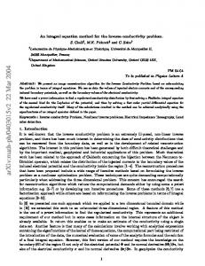
A FIG. 2. Plot of (x or (I~ vs A=&/d for a symmetrical ET reaction in a Debye solvent with T= 10 ps, AG”=O.O, and @co = 1 ps-‘. The middle curve shows the empirically determined values aD used in the improved double-exponential formula that provides a good fit to the integral equation solutions-see Fig 3. The upper curve for (x is calculated from JZq. (4.3a) and the lower curve for a, from Eq. (4.21).
(4.14)
-K-t).
-K+
0-l 0.0
--2~~=-B’f[B’~-4+(k;,+k;,)]‘”
(4.18)
It is easily verified that when t=O, Q2(t) =0, and that as t-+ CO, Q,(t) -+k,J(k,,+ k2J which is its equilibrium value. In the limit A+O, Eq. (4.13) becomes identical to the single-exponential formula characteristic of the wide reaction window limit (Sec. II) when one finds K+ =k,, =kl and C- =O. A similar limit (K+ =kle) is reached in
(4.23)
and (4.24) where B’ = B,/a,. One easily verifies again that Q,(t) =O when t=O, and that Q2(t)-fkl/(kl,+k2J as t+ CO. FA (7) already reflects the complex solvation dynamics of non-Debye solvents. The double-exponential form may
J. Chem. Phys., Vol. 98, No. 2, 15 January 1993
Downloaded 05 Jun 2004 to 130.111.64.68. Redistribution subject to AIP license or copyright, see http://jcp.aip.org/jcp/copyright.jsp
J. Rasaiah and J. Zhu: Reversible electron-transfer
1221
reactions
TABLE III. The empirically determined correction factor (~a and rate constants for the doubleexponential interpolation formulas describing electron transfer in Debye solvents when TV= 10 ps, AGc=O and #Ice = 1 ps-’ as a function ofA=&//l.
A 0.999 0.909 0.833 0.667 0.500 0.200
QD
C,’
5.5 3.30 2.50 1.5 1.28 1.06
-0.4443 -0.419 -0.4050 -0.3737 -0.355 -0.335
TLK:
TLK,-
0.1829 0.2249 0.2512 0.3104 0.3629 0.4114
2.271 2.936 3.322 4.007 3.472 3.322
c;
-0.0557 -0.0803 - 0.0949 -0.1263 -0.1442 -0.1648
thus be extended to non-Debye solvents by replacing TV by qnit or by assuming an effective relaxation time [Eq. (2.13)]. The general accuracy of the last assumption (see Sec. VI) may not be good. Another method of solving the integral equation for ET in non-Debye solvents assuming an effective relaxation time 72 has been presented elsewhere2 to which the reader is referred. The correction factors a and aD which modify the thermal equilibrium rate constants kie in the singleexponential interpolation formula and improved doubleexponential formulas enable the survival probabilities to be predicted not only in the different limits, but also in the regions between them. When a or ag is significantly greater than unity, the electron-transfer rate is controlled by the solvation dynamics. Figure 2 shows that this occurs as A approaches the narrow window limit when the dynamics of the outer solvation sphere plays an increasingly significant role in the kinetics of electron transfer. Although Eq. (4.3a) for a is qualitatively correct, its accuracy is limited by the approximations used in deriving it (see the Appendix). In Fig. 2 we plot a and aD vs A for a symmetrical electron-transfer reaction (AGa=O) in a Debye solvent assuming rL= 10 ps and @ko = 1.0 ps-‘. Note that aD < a and both a and aD+ 1 when r=-+O. On
Q,0) 0.9
~~=lOps,dj?k,=
Ips-I,
pAGo=
.o
r&a
0.2077 0.3302 0.417 0.622 0.630 0.683
comparing the improved double-exponential form with the solutions to the integral equations that are discussed in Sec. V, we find that aD calculated from Eq. (4.21) is a little too small above A=O.S. Values that give a better fit to the integral equation solutions at longer times can be determined empirically; they are also shown in Fig. 2. Table III contains the corresponding rate constants and coefficients obtained in this way and Fig. 3 displays results that are quite typical. It is seen that the agreement with the integral equation solutions is excellent at long times but less so at very short times. Since ag is strongly correlated with the reaction parameters ( AGe, etc. ), the values displayed in Table III are accurate only for the particular reaction considered. In the discussions that follow in Sec. V, the survival probabilities in the improved double-exponential approximation are calculated using Eq. (4.22) for aD The analytic expressions discussed here (double- and singleexponential time dependencies) are also useful in deducing the approximate functional forms of the numerical solutions to the integral equations described in the next section.
V. NUMERICAL SOLUTION TO THE INTEGRAL EQUATIONS The solutions discussed in Sets. III and IV are limiting cases or approximations to the integral equations. No general analytic solution in the time domain is possible except in special cases and the solution, especially for systems with multiple relaxation times, has to be obtained numerically. This can be done in small time increments starting from the initial condition at zero time as follows. Let t=mt’ and u=nt’, where t’ is the time step and m and n are integers with man. Using the trapezoid rule and the initial condition Q,(t) = 0, we have, at the first time step Cm= 11, Q,2) Q,(mt’> =klet’FIG. 3. Comparison of the survival probabilities after ET calculated from the integral equation and the double exponential approximations. The system parameters are AJ&=O.2, TV= 10 ps, @.=5, @kc = 1 ps-‘, and gAGa=O.O. The curves are identified as follows: (-----) integral equation; (-+-) double-exponential approximation; (---- X ----) improved double-exponential approximation (aD=2.5).
(P/2)
a(O)Q,(mt’)
m-1
+2
2 a[(m-n>t’lQ2W>
n=l
Solving for Q2(mt’),
.
(5.2)
and making use of Eq. (5.1), we get
J. Chem. Phys., Vol. 98, No. 2, 15 January 1993 Downloaded 05 Jun 2004 to 130.111.64.68. Redistribution subject to AIP license or copyright, see http://jcp.aip.org/jcp/copyright.jsp
1222
J. Rasaiah and J. Zhu: Reversible electron-transfer
7.00
+N3JxE5 0
TL= lops,flk,= jps-‘, BAG’=-1.0
1W
I
~. .-;-;:;‘-
y* s7J2 for small enough s. It follows that in the long-time limit, asi(s) z=kie(rLfA+
l/s),
(-44)
where (A5) When A = 1 (narrow window limit), explicit summation shows’ that fA--,0.6. Since OgA-kiez
2~
(A17a)
where
(A17b)
(A91 As A + 0, FA ( G-)-t 0. For Debye solvents FA ( T) =q$,+
ai=ko[(l+A)/(243’2)]exp[~i(A-l)][1
-erf( &)I, 2. Short-time
We first discuss the short-time behavior in Debye solvents before discussing the same limit in non-Debye solvents. At short times t