United States Air Force Academy, USAF Academy CO, USA .... was established by US Air Force Research Labs, who offered the configuration for studies to ...
AIAA 2010-4392
28th AIAA Applied Aerodynamics Conference 28 June - 1 July 2010, Chicago, Illinois
An Integrated Computational/Experimental Approach to UCAV Stability & Control Estimation: Overview of NATO RTO AVT-161 Russell M. Cummings* United States Air Force Academy, USAF Academy CO, USA Andreas Schütte† German Aerospace Center (DLR), Braunschweig, Germany
A comprehensive research program designed to investigate the ability of computational methods to predict stability and control characteristics of realistic flight vehicles has been undertaken. The integrated approach to simulating static and dynamic stability characteristics for a generic UCAV and the X-31 configuration was performed by NATO RTO Task Group AVT-161. The UCAV, named SACCON (Stability and Control Configuration), and the X-31 are the subject of an intensive computational and experimental study. The stability characteristics of the vehicles are being evaluated via a highly integrated approach, where CFD and experimental results are being used in a parallel and collaborative fashion. The results show that computational methods have made great strides in predicting static and dynamic stability charactersitics, but several key issues need to be resolved before efficient, affordable, and reliable predictions are available.
Nomenclature a
=
Acoustic speed [m/s]
n
=
Yaw moment [N-m]
b
=
Wing span [1.538 m]
p
=
Pressure [N/m2]
cr
=
Root chord [1.0608 m]
q
=
Dynamic pressure [N/m2], ≡ ρV / 2
cref
=
Reference chord [0.479 m]
s
=
Wing half span [0.769 m]
Cl
=
Roll moment coefficient, ≡ l /( q∞ Sb )
S
=
Wing reference area [m2]
CL
=
Lift coefficient, ≡ L /( q∞ S )
V
=
Velocity [m/s]
Cm
=
Pitch moment coefficient, ≡ m /( q∞ Scref )
x
=
Chordwise coordinate [m]
2
Cn
=
Yaw moment coefficient, ≡ n /( q∞ Sb )
y
=
Spanwise coordinate [m]
Cp
=
Pressure coefficient, ≡ ( p − p∞ ) / q∞
Y
=
Side force [N]
CY
=
Side force coefficient, ≡ Y /( q∞ S )
z
=
Vertical coordinate [m]
l
=
Roll moment [N-m]
α
=
Angle of attack [deg]
L
=
Lift [N]
β
=
Angle of sideslip [deg]
m
=
Pitch moment [N-m]
ρ
=
Density [kg/m3]
M
=
Mach number, ≡ V / a
θ
=
Pitch angle [deg]
∞
=
Freestream condition
* †
Professor of Aeronautics, Department of Aeronautics. AIAA Associate Fellow. Research Engineer, Institute of Aerodynamics and Flow Technology. 1 American Institute of Aeronautics and Astronautics
This material is declared a work of the U.S. Government and is not subject to copyright protection in the United States.
I. Introduction
S
TABILITY and control (S&C) engineers have used an iterative process combining semi-empirical lower-order, wind-tunnel, and flight test modeling techniques to determine the aerodynamic characteristics of new fighter aircraft. Despite their greatest efforts using the best available predictive capabilities, nearly every major fighter program since 1960 has had costly nonlinear aerodynamic or fluid-structure interaction issues that were not discovered until flight testing. 1,2,3,4,5 Some examples include the F-15,6 F/A-18,6 F/A-18C,7 AV-8B,6 and the B-2 Bomber.8 The F-15, F/A-18A, and AV-8B all exhibited significant aero-elastic flutter,6 while the F/A-18C experienced tail buffet at high angles of attack due to leading-edge extension vortex breakdown,7 and the B-2 Bomber experienced a residual pitch oscillation.8 The development costs of each of these aircraft could have been drastically reduced if these issues had been identified earlier in the design process. Clearly, a high-fidelity tool capable of reliably predicting and/or identifying configurations susceptible to handling quality instabilities prior to flight testing would be of great interest to the S&C community. Such a tool would be well suited to the aircraft design phase and would decrease the cost and risks incurred by flight-testing and post-design-phase modifications. Several tools can be used to predict the S&C characteristics of an aircraft, including flight and wind tunnel testing, semi-empirical lower-order modeling and computational fluid dynamics (CFD). Flight testing is the most accurate of these methods, but is also the most expensive and cannot be used during early stages of the aircraft development process because the aircraft configuration typically is not finalized. Wind tunnel testing is also accurate, but suffers from scaling issues, along with difficulty modeling unsteady dynamic behavior. Wind tunnel testing is also expensive, although cheaper than flight testing. Semi-empirical lower-order modeling has less fidelity than flight and wind-tunnel testing and is incapable of reliably predicting unsteady nonlinear aerodynamic behavior. A reasonable compromise between flight and wind tunnel testing and semi-empirical lower-order modeling is CFD simulation. Modern CFD techniques have a relatively high level of fidelity and have successfully modeled the nonlinear aerodynamic behavior of aircraft at full scale Reynolds numbers. This method reduces some of the major uncertainties associated with sufficiently modeling physical space. However, it comes with an additional cost in execution time that results from computer performance and small physical time step requirements to accurately capture the flow physics. This is exaggerated by the low frequency nature of most of the aerodynamic motions that result in nonlinear behavior of interest. Researchers at NASA Ames, for example, have attempted to perform a “brute force” approach to filling a stability and control database for vehicle design.9,10,11 They found that a reasonable database for static stability and control derivatives would include on the order of 30 different angles-ofattack, 20 different Mach numbers, and 5 different side-slip angles, each for a number of different geometry configurations or control surface deflections.9 They envisioned that a few hundred solutions can be obtained automatically and the remainder of the parameter space is filled using an interpolation procedure or neural networks. Considering today’s performance of computers and CFD codes, the routine calculations of hundreds of maneuvers in a reasonable time frame is unrealistic. In order to accurately and reliably predict the stability and control characteristics of an aircraft prior to the costly flight test phase, CFD has to be combined with predictive modeling of lower complexity. The vision of using CFD in the initial aircraft design phases initiated several projects within S&C, CFD, and wind tunnel communities, including Computational Methods for Stability and Control (COMSAC)3 and Simulation of Aircraft Stability and Control Characteristics for Use in Conceptual Design (SIMSAC). These groups have met with varying degrees of success, and also helped to formulate the creation of a NATO Research & Technology Organization (RTO) group that would investigate some of these issues.
II. AVT-161 Task Group The NATO RTO AVT-161 Task Group was established to determine the ability of computational methods to accurately predict both static and dynamic stability of air and sea vehicles. Whereas this paper will concentrate on the air vehicle application within the Task Group, the overall approach is to identify major synergy in terms of physical modeling, fluid structures, or transition effects. The Task Group joins three major avenues of interest: the experimental part to provide highly accurate static and dynamic validation data; the CFD community who, is trying to predict the steady state and dynamic behavior of the target configurations; and the S&C group which is analyzing the experimental and numerical data. The objective of the group is to provide best practice procedures to predict the static and dynamic behavior especially for configurations with vortex-dominated flow fields where non-linear effects have a significant impact. These non-linear regimes are the areas where typical linear S&C methods fail, or where wind tunnel data are only available for non-full-scale flight flow regimes. Currently these deficiencies can only be addressed through costly flight testing. Because of this the main focus is the prediction with CFD methods rather than enhancing existing S&C system identification methods. The AVT-161 Task Group partners and their contributions are listed in Table 1.
2 American Institute of Aeronautics and Astronautics
A. Background AVT-161 began as an outgrowth of previous RTO Task Groups which also investigated the ability of CFD to predict complex aerodynamics. These previous groups (AVT-080 and AVT-113) studied the ability of various CFD prediction methods (including Euler and Navier-Stokes prediction) to accurately predict vortical flows on vehicles at medium to high angles of attack. AVT-080 focused on determining the ability of CFD to predict vortical flow structures on delta wing.12,13,14,15 In AVT-11316,17 the focus was on experimental and numerical investigations on delta wing configurations with various leading edges from sharp to different round radii. AVT-113 started from given fundamental wind tunnel data by NASA18 followed by several pre-test CFD results which supported the wind tunnel investigations with advanced experimental methods. All of these investigations resulted in improved understanding of the flow physics and new best practice methods for computational simulation of vortical flows. The results of the AVT-113 Task Group have been presented at the AIAA conference in 2008 within an experimental19,20,21,22,23 and numerical sessions.24,25,26,27,28,29,30,31 The second target configuration of the AVT-113 Task Group was the F-16XL CAWAPI configuration. A special section of the Journal of Aircraft also included several papers by Lamar and Obara,32 Boelens et al.,33,34 Görtz et al.35 and Fritz et al.36 A summery of lessons learned is given by Rizzi et al..37 Since the overall goal of AVT-161 was to determine the ability of modern CFD tools to adequately predict static and dynamic S&C parameters for modern aircraft, two candidate configurations were chosen: a generic UCAV (Stability And Control CONfiguration, SACCON) and the X-31. Both AVT-161 Task Group target configurations possess a delta wing planform with medium sweep leading edges (between 45° and 57° sweep angle), and with leading edge nose radii varying from sharp to medium and large roundness. The approach is to provide most (if not all) flow features common to typical UCAV and fighter aircraft configurations, and to investigate the aerodynamic challenges which have to be captured by computational methods. There are several investigations in the past focused on the prediction of UCAV/delta wing configurations in maneuvering flight. Recent experimental and CFD investigations of the dynamic behavior of a pitching UCAV configuration is given by Cummings et al.38 as well as investigations on time dependent flow predictions.39 The dynamic aerodynamic effects on the vortical flow of pitching and rolling delta wings are discussed in several references: numerical investigations are given by Ericsson40 and Arthur et al.,41 whereas experimental investigations are given by Chaderjian and Schiff,42,43 Hanff et al.,44 and Hummel and Löser.45 The unsteady PIV approach applied on a rolling delta wing is given by Sammler et al.46 Within a DARPA project several experimental investigations on aerodynamic structural mechanics coupling effects are analyzed by wind tunnel tests using a UCAV model configuration. These results can be found in Kudva and Sanders et al.47 Another issue which is relevant for former and recent research concerning delta wing configurations in maneuver flight is the occurrence of laminar regions. A recent contribution to this topic is given by Arthur et al.48 The CFD prediction of the laminar/turbulent transition of a UCAV configuration is discussed. Another important previous project covering experimental and numerical aerodynamic behavior of UCAVs is the investigation using the 1303 UCAV configuration. The 1303 configuration was established by US Air Force Research Labs, who offered the configuration for studies to other partners and for the UK. The 1303 configuration is a tail-less “flying-wing” with a leading-edge sweep angle of 47°. Among others, the publications of Zhang et al,49 Petterson,50,51 Wong,52 Arthur,53 and Sherer et al.54 should be mentioned. The X-31 configuration was also chosen for AVT-161 as a challenging test case for CFD. The X-31 has been used as a target configuration within the DLR Project Sikma – “Simulation of complex maneuvers”.55,56,57 Within the DLR project several experimental and numerical investigations were established. Based on these investigations, additional wind tunnel tests were done by DLR to complete the data set and exapnd the knowledge of the wind tunnel model aerodynamic characteristics. All of these results were used within the AVT-161 Task Group. B. Experimental/Computational Integration Experimental and computational investigations have not always been conducted in the most advantgeous or efficient manner in the past. Often these programs are done separately or in parallel with little or no integration. An overview of typical ways experiments and computations are used in research programs was reviewed previously and discussed.58 Some notable exceptions to the inefficient approach of the past have been the European helicopter project GOAHEAD59 and Project EPISTLE.60 In an attempt to insure that the computational requirements for the experimental data were included in the planning as the Task Group progressed, the CFD participants were asked early in the program to identify a “wish list” of experimental results. The over-arching theme of the responses can best be summarized as: understand the developing flow structures. In other words, the CFD community not only wanted to know the gross aerodynamics of the vehicle, but also the causes of any interesting/unusual flow phenomenon. This request was nearly unanimous and quite strongly stated by the CFD members, and the experimental researchers kept the requests in mind as they designed the wind tunnel tests. Here is the list of requests, in no specific order:
3 American Institute of Aeronautics and Astronautics
1.
2.
3. 4.
Have at least two to three tunnel entries (possibly in multiple tunnels) so that the following can be accomplished: a. measure static aerodynamics first (at various angles of attack and sideslip, with and without control surface deflections) so that the CFD community can begin to understand the details of the flow and have a chance to validate our predictions and aid in defining the parameters for the follow-on tunnel entries b. measure dynamic derivatives and/or perform dynamic maneuvers—there was a large variation of ideas here, but we can certainly discuss this in Athens; the model scale needs to be appropriate for realistic reduced frequencies and for multiple wind tunnels It is essential to accurately know and verify the tunnel conditions, including: a. freestream conditions, including flow angularity and variability b. tunnel wall effects c. model deformation d. model position in the tunnel It is also essential to know the experimental uncertainty for all measured quantities for both static and dynamic testing. Important results should be repeated to aid in this knowledge. Besides forces/moments and surface pressures, the following flow visualization suggestions would help the CFD community a great deal: a. knowledge of flow near the leading edge, trailing edge, and wing tips b. unsteady surface measurements, including surface pressures and flow patterns (accomplished with pressure transducers, surface oil flows, and/or PSP) c. knowledge about transition locations d. unsteady flow field measurements, including knowledge about vortex development and interactions via off-surface flow visualization (accomplished with PIV and/or LDA)
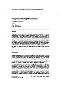
The CFD researchers realize that they were asking for “everything”, but strongly believed that in order to truly understand the developing flow field about the UCAV configuration a great deal of information would be required. They also realized that some of this information would be difficult (or even impossible) to obtain, but those situations would be discussed and achieved as the plan progressed. The overall requirements and goals for the group having been set, the SACCON configuration research project took place acoording to the timeline shown in Figure 1. Initial planning for the Task Group took place during 2007, resulting in a proposal of the SACCON configuration in Fall of 2007 by DLR and EADS-MAS. That initial design was examined with both lower-order modeling and CFD during the last half of 2007, during which time it was determined that the design could be improved with some relatively minor re-design changes, which took place during the first two months of 2008 with inputs from EADS-MAS, BAE Systems, and DLR, with parallel configuration design studies done by Nangia Consulting. Once the redesigned configuration was finalized, detailed test planning began by DLR and German-Dutch Wind Tunnels (DNW) for two entries in the DNW-NWB wind tunnel. This was accompanied in parallel by numerous static CFD simulations being conducted by DLR, EADSMAS, NASA Langley, and the US Air Force Academy. Other CFD static simulations were completed prior to the end of wind tunnel testing by the University of Liverpool, FOI, DSTL, DSTO, NLR, Metacomp, and ONERA. Lower-order model estimates of the static aerodynamics were also conducted by Nangia Consulting and NEAR. The ability of these various approaches to predict the static and dynamic behavior of the SACCON configuration forms the foundation of the purpose of the Task Group. The first campaign in the DNW-NWB tunnel included force and moment testing of both static and dynamic cases. Once this data was available a number of organizations began performing dynamic simulations using CFD including NLR, DLR, NASA Langley, and the US Air Force Academy. The simulations were being conducted at the same time the second campaign took place in the DNW-NWB tunnel, which was primarily to perform flow visualization studies. PIV measurements were made by both DLR and ONERA, and this off-surface flow information will form a crucial part of understanding the flow field and resulting forces and moments of SACCON. In addition, initial analysis of the stability and control characteristics of SACCON has already started and will continue in parallel with the CFD simulations and the additional wind tunnel test being planned for the end of 2009 at NASA Langley in the 14′×22′ wind tunnel. The timeline in Fig. 1 shows how an integrated approach to a fairly complex design/compute/test program can be conducted in a relatively compressed time schedule. The progress made to date is even more impressive when taking into account the nature of this program, since it is a RTO Task Group and not the primary job of the participants of the group. The interaction between predictions and experiments has already shown a great deal of value, since the predictions showed some of the problems with the initial design and greatly aided in the redesign of the configuration. Also the predictions aided in the wind tunnel test planning and provided estimates of loads for model design and areas of interesting aerodynamics for test scheduling. The comprehensive data collected proved invaluable to the researchers performing predictions, and greatly helped to accomplish the initial goals of the group: 4 American Institute of Aeronautics and Astronautics
to understand the developing flow structures and be able to accurately predict them for stability and control purposes.
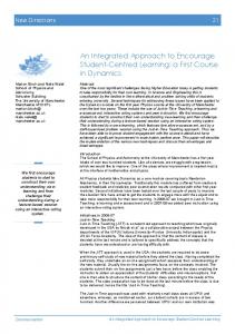
III. Configurations and Wind Tunnel Models Within the AVT-161 Task Group two highly swept wing configurations are used for experimental and numerical investigations. The DLR X-31 wind tunnel model configuration is a double delta wing configuration with canard. The inner delta wing has a sweep angle of 57° and the outer 45°. The canard is a cropped delta wing with a sweep angle of 45°. Additional characteristics of the model are the inner and outer leading edge flaps, the trailing edge flaps, the front wing and rear fuselage strakes as well as the tail plane with rudder. The investigations within the AVT-161 Task Group are done without any control device deflection but taking the stream wise gaps between the leading edge flaps into account. The X-31 wind tunnel model configuration on the MPM system is shown in Figure 2. The main target configuration of the Task Group is a generic UCAV geometry called SACCON. The planform and section profiles were defined in cooperation between DLR and EADS-MAS. DLR adjusted the pre-design geometry for wind tunnel design purposes which actually lead into a higher overall thickness at the root chord to provide enough space for the internal strain gauge balance. Finally the wind tunnel model was designed and manufactured within the responsibility of NASA at NASA Langley Research Center. The model mounted on the MPM system in the low speed wind tunnel Braunschweig (DNW-NWB) is shown in Figure 3. The SACCON UCAV has a lambda wing plan form with a leading edge sweep angle of 53° (see Figure 4 and 5). The root chord is approximately 1m and the wing span is 1.53 m. The main sections of the model are the fuselage, the wing section and wing tip. The configuration is defined by three different profiles at the root section of the fuselage, two sections with the same profile at the inner wing, forming the transition from the fuselage to wing and the outer wing section. Due to radar signature issues the leading edge is parallel to the wing trailing edges and the wing tip is designed parallel to the trailing edge of the fuselage section. Finally the outer wing section profile is twisted by 5° around the leading edge to reduce the aerodynamic loads and shifting the onset of flow separation to higher angles of attack. The wind tunnel model consists of different modular parts. The leading edge is exchangeable providing a sharp (SLE) and a variable round leading edge (RLE). The RLE is sharp at the root chord and the leading edge radius is growing in span wise direction up to the intersection between fuselage and wing and decreasing again. The overall radius distribution and relative thickness of the RLE configuration is given in Figure 6. Furthermore the wing tips can be separated and the rear part of the wing section is prepaired to add control devices. The model is made of CFRP and is very light with an overall weight of less than 10kg (including pressure tubes and PSI modules). The very light design reduces the dynamic inertia loads enabling the use of a smaller, more sensitive balance that provides better force and moment resolution. The model was designed to accommodate a rear sting or belly sting mount for tests in the DNW-NWB low speed facility at DLR in Braunschweig and the 14′×22′ low speed wind tunnel at NASA LaRC. Different connection links between belly sting support and internal balance at NWB provide an angle of attack range from 15° to 30°. This is provided by two different rigid cranked yaw links or by using an internal pitch link driven by a 7th axis. The two different basic setups with and without 7th axis are shown in Figure 7. The position of the belly sting connection is chosen to minimize the influence of the sting on the overall flow topology. This applies mostly to the vertical flow on the upper side of the model. This influence has to be approved via CFD simulations. Out of previous investigations with the X-31 configuration it was shown that for the prediction of the total forces and moments the sting support has to be taken into account.57 It can be seen in Fig. 6 that the connection between sting support and internal balance is completely covered by the model fuselage for the configurations with yaw link. These are adapted new designs especially for the SACCON configuration. For the pitch link it was not possible to adapt the design and a cover was used to smooth the geometry in this area. The SACCON wind tunnel model is equipped with more than 200 pressure taps on the upper and lower side of the model. The taps are connected with pressure tube to PSI modules within the model. At nine additional positions unsteady pressure sensors are mounted. The location of the pressure taps is depicted in Figure 8. The pressure tap locations result from preliminary CFD computations prior to the wind tunnel tests. The aim was to capture the complex vortex flow topology over the configuration and operation points of the trajectory. One of these simulations results are seen as well in Fig. 7. The preliminary simulations based on best practice procedures resulting from CFD prediction of configurations with round leading edges like results from AVT-113.31 All pressure tube connections between the pressure taps and PSI modules are of the same length to guarantee the same time dependent behavior for each pressure taps during the unsteady pressure measurements. This leads to big bundles of the flexible tubing which have to be carefully installed to prevent kinks. The tubes bundles which have to be placed inside the model are shown in Figure 9. The surface finish of the model was motivated by PIV measurement
5 American Institute of Aeronautics and Astronautics
requirements. The shiny black paint contains particles of Rhodamine B, which reflects light that consists of a different wave length which can be filtered. This leads to a highly accurate PIV measurement close to the surface. Initial tests with the RLE configuration showed an arbitrary transition line on the upper surface of the model detected by infrared thermography. These measurements lead to the decision to prepare the leading edge with a carborundum grit trip as it is depicted in Figure 10. The difference between the configuration with and without transition tripping is shown in Figure 11. On the left hand side the clean configuration with no tripping at the round leading edge and an arbitrary transition line between laminar and turbulent flow can be observed. On the right hand side the infrared thermography picture after the installation of the carborundum grit trip is shown. It can be observed that after establishing the grit a fully turbulent flow over the upper wing surface can be assumed.
IV. Experimental Approach The following section describes the wind tunnel facilities used for establishing the steady state and dynamic experimental data for the X-31 and SACCON configuration. The first part of the SACCON tests was conducted in the Low Speed Wind Tunnel Braunschweig (DNW-NWB) which is part of the foundation of “German Dutch Wind Tunnels”. The second part of SACCON tests was done at NASA Langley Research Center (LaRC) in the 14′×22′ low speed wind tunnel facility. Finally, the Defense Science and Technology Organization (DSTO) in Australia performed some basic research focused on vortical flow structures and derivatives with a small scaled model in a water tunnel. A. Wind and Water Tunnels 1. Low Speed Wind Tunnel Braunschweig (DNW-NWB) The DNW-NWB belongs to the foundation “German–Dutch Wind Tunnels” under Dutch law. DNW operates 12 different wind tunnels on five sites in Germany and the Netherlands. The DNW-NWB is located on the DLR site in Braunschweig, Germany. It is a closed-circuit, atmospheric type wind tunnel, which can be operated either with an open, slotted or closed test section. A plan view of the tunnel is given in Figure 12. The test section size is 3.25m by 2.8m (10.6ft by 9.2ft). The maximum free stream velocity is V = 80 m/s (263 ft/s) in the closed test section and V = 70 m/s (230 ft/s) in the open test section. High performance secondary air systems (compressors and vacuum pumps) allow for tests featuring turbine power simulation (TPS) or engine intake tests. NWB’s model supports include basic α-β-support, half-model support, support for 2D-models, a rotary motion support for rolling and spinning tests and the Model Positioning Mechanism (MPM), which will be described in more detail in section B. 2. NASA Langley 14′×22′ Low Speed Wind Tunnel The forced oscillation test rig in the NASA Langley 14-by-22-Foot Subsonic Tunnel (shown in Figure 13), can provide constant amplitude and frequency sinusoidal motion in the roll yaw or pitch axes.61 The frequency can be set from 0.1 to 1.0Hz at amplitudes up to 30 degrees. The SACCON model completed roll and yaw oscillation tests in this tunnel in the fall of 2009. The yaw oscillation testing repeats some of the conditions tested in the DNWNWB Low Speed Tunnel for test to test comparison. 3. DSTO Water Tunnel The DSTO water tunnel is an Eidetics Model 1520 tunnel. The tunnel has a horizontal-flow test section 380 mm wide, 510 mm deep (15 x 20 inches) and 1630 mm long. It is a recirculating closed-circuit tunnel with a 6:1 two dimensional contraction. The freestream velocity in the test section can be varied between 0 and 0.6 m/s. Models are mounted on a C-strut so that the required centre of rotation of a model is at the centre of the imaginary circle formed by the strut, ensuring that all angular motion of the model is about this point. The SACCON water tunnel model has a span of 250 mm and the wind tunnel model spans 1538 mm, resulting in a model size ratio of 6.15:1. The Reynolds number of the water tunnel model ≈ 8000, for U = 0.1 m/s. Mechanism DNW-NWB’s Model Positioning Mechanism is a six DOF parallel kinematics system designed for static as well as for dynamic model support. Characteristic features of this unique test rig are the six constant length struts of ultra high modulus carbon fibre and the six electric linear motors, which move along two parallel rails. The first Eigenfrequency at the MRP is above 20 Hz. The MPM is located above the test section and can be operated in the open test section as well as in the closed one. The location of oscillation axes can be chosen arbitrarily and in addition to classic sinusoidal oscillations the MPM can perform multi-DOF maneuvers. An artist’s impression of the MPM carrying the SACCON model in the open test section is given in Figure 14. More details concerning the MPM are given in Bergmann et al.62,63
6 American Institute of Aeronautics and Astronautics
C. Measurement technique 1. Transition Because the precise knowledge of the flow conditions is of paramount importance for tests, which are used for CFD validation, the wind tunnel entry was begun with boundary layer transition observations using infra red thermography. In case the model surface and the passing air have different temperatures, the transition line can be observed with an infra red camera of suitable sensitivity because of the different heat transfer properties of laminar and turbulent boundary layers. The DLR Institute of Aerodynamics and Flow Technology utilizes a set of cameras on remotely controllable mounts for this purpose since more than a decade. Typical results are given in Fig. 10. 2. Forces and Moments For the measurements of forces and moments internal six component strain gauge balances have been used. The X-31 wind tunnel models have been equipped with an Emmen 192-6 balance, whereas the SACCON model has been instrumented with a smaller Emmen 196-6 balance. 3. Pressures The X-31 wind tunnel models are equipped with 54 in situ mounted Kulite pressure transducers. To permit pressure measurements on DNW-NWB’s rolling and spinning support the transducers are of the absolute pressure measurement type. The Kulites are not installed permanently but can be dismounted, so one set of transducers can be used for both X-31 wind tunnel models. For the SACCON wind tunnel model a combination of in situ mounted Kulite pressure transducers and 48-channel ESP modules, mounted in the model’s center section have been used. The Kulite transducers have been installed to verify the synchronicity of the ESP modules with respect to balance and position data acquisition. The signals of the ESP modules have been corrected for attenuation and phase shift according to Nyland et al.64 4. Model Position For the measurement of the instantaneous attitude and position of both X-31 and SACCON wind tunnel models DNW-NWB employed an optical system featuring two high speed video cameras. The cameras have been mounted below the test section and acquire SXGA (1280x1024) images at 300 frames per second, each. The position of the model is calculated in real time from the pixel co-ordinates of three markers, which have been applied to the model surface. For static angle of attack measurement a conventional inclinometer has been installed additionally. Two different data acquisition systems have been employed for force and pressure measurements in the X-31 tests on the one hand and the SACCON tests on the other hand. The X-31 test has been performed with a telemetric system consisting of 64 channels with a 16 bit resolution. The SACCON test has been made with DNW-NWB’s standard Hottinger-Baldwin MGC+ data acquisition. 5. PIV- “Particle Image Velocimetry” Three component PIV measurements have been performed on the SACCON wind tunnel model in the DNWNWB by teams of ONERA and DLR simultaneously. Cameras and laser light sheets have been installed outside the test section without direct mechanical contact to the test section structure in order to avoid quality reduction due to vibration. Optical access was granted by windows in the test section side walls, as can be seen in Figure 15. Cameras and laser light sheets were aligned parallel and orthogonal to the model’s x-axis at an angle of attack of α = 17°, as the force and pressure measurements indicated that an angle of attack range between 14° and 20° offers the most interesting and challenging flow topologies for CFD. The ONERA PIV setup was oriented towards the front part whereas the DLR PIV setup was oriented toward the model’s rear part. Employing the MPM’s capabilities, the model was displaced along its x-axis in order to move the light sheets along the model. This eliminated the need for time consuming re-calibrations of the cameras when the location of the light sheet relative to the model was changed. While most of the PIV measurements have been made on the right hand side of the model, the DLR team also made measurements on the left hand side. Figure 16 illustrates the locations of the PIV light sheets on the SACCON model. The DLR PIV team used 300 images from each camera. The ONERA team used 800 images. The ONERA cameras had a higher resolution than the DLR cameras but the oberserved area was smaller. A typical PIV result is given in Figure 17. In addition to the static PIV measurements also measurements on the model oscillating in pitch have been performed. The PIV cameras were triggered in a phase locked mode by the model oscillation. PIV data are taken at eight different phase angle over the oscillation cycle. For each phase angle fifty measurements ate taken averaging. D. Wind tunnel tests Within AVT-161 two additional wind tunnel campaigns with the X-31 configuration in the open test section of the DNW-NWB were done. The first test focused at the influence of the model setup on the integral data and 7 American Institute of Aeronautics and Astronautics
pressure distribution on the model. For instance the influence of the sting support, influences of gaps between the support and the model as well as on flap gaps and elastic effects at the hinge line of the leading and trailing edge flaps. In Figure 18 the different setups related to the leading edge flap gaps are depicted. Three different setups where tested: All gaps sealed, all gaps open and only the span wise gaps sealed between the LE-flaps and the wing. The results for five different angles of attack are shown in Figure 19. It can be observed that there are significant differences in the pressure distribution for all three setups. This is caused by the fact that the vortex formation is very sensitive to the setup at the LE. This effect has a minor influence on the overall lift but has significant influence on the longitudinal and lateral stability. The influence of the belly sting on the pitching moment is shown in Figure 20. In Fig. 20 the pitching moment verses the AoA is plotted. It can be observed that the additional 7th axis behind the belly sting causes a parallel shift to higher values which causes a rear loading in comparison to the setup without 7th axis. A comparable setup can be seen in Fig. 7 for the SACCON configuration. The result from the first X-31 test led to the final configuration setup of the model and support for the second wind tunnel entry. In the second wind tunnel entry steady state and unsteady experimental data have been obtained. The dynamic tests include sinusoidal pitch and yaw motion. These data were finally used for computer code validation purposes. First results of these investigations are described by Boelens 65 and Jirasek & Cummings.66 Two examples of the maneuvers which have been performed are shown in Figure 21. The red curve shows the AoA versus time of an overlay pitching maneuver. The MPM establishes the slower movement with high amplitude whereas the 7th axis is used to overlay the higher frequency motion with smaller amplitude. With the SACCON configuration two wind tunnel tests in the closed test section of the DNW-NWB are done up to now. A third test will follow at the end of 2009 in the 14ft×22ft low speed wind tunnel at NASA LaRC to complete the experimental investigations. The first tests focused on the identification of the basic aerodynamic behavior of the SACCON configuration. The tests were done with three different belly sting setups. Due to the experiences of the X-31 tests two different belly sting supports are established to reach higher angles of attack without the influence of a 7th axis behind the sting. Nevertheless there is an influence of the support left just by changing the crank angle between the sting and the model by 15°, as seen in Figure 22. Fig. 22 shows as well the different angle of attack ranges which can be achieved by using the one or the other yaw link setup. Figure 23 shows the influence using the pitch link with 7th axis instead of the 15° cranked yaw link, see as well Fig. 7. Whereas in Fig. 20 and Fig. 22 only a parallel shift of the pitching moment coefficient can be observed due to a change of the setup, is the influence of the 7th axis setup in Fig. 23 is different. This different behavior is probably caused by the additional cover between the sting and the model fuselage. Figure 24 and 25 should show the aerodynamic characteristic behavior of the SACCON configuration itself. In Fig. 24 the lift and pitching moment coefficient versus AoA for sharp LE, round LE and round LE with fixed transition is shown. It can be seen that the overall lift is fairly the same for all kinds of leading edges. Only the curve of the sharp leading edge configuration shows a higher lift at angles of attack above 12°. This is caused by the higher nonlinear component of lift due to stronger vortices which occur at the sharp leading edge. The pitching moment coefficient shows much more sensitivity due to the change of the LE shape. The characteristic discontinuous behavior between AoA of 10° and 20° takes place earlier for the sharp leading edge as for the two round leading edge configurations. Fig. 23 shows as well a significant different pitching moment distribution between the RLE and RLE-FT configuration. The reason for this behavior is to some extent already explained by the Task Group taking experimental data and CFD results into account. The discussion of these results should not be part of this publication and will be delivered later. Fig. 25 shows the behavior of the SACCON configuration at non-symmetric on flow conditions. It is seen that at angles of attack higher than 10° (depending on the direction of the angle of sideslip) significant differences can be observed. Even at small angles of side slip this non-symmetric behavior can be seen. To ascertain the flow causing these flow conditions is part of the Task Group and one major issue of the code validation process to get the ability to predict seriously the stability and control issues of the target configurations. All the discussed parameters above have to be taken into account when preparing the computational simulations. Further boundary conditions are, among others, the condition of the model surface (taped screws and gaps, surface roughness), transition effects, as discussed before in Chapter III, and the wind tunnel corrections. A wind tunnel test in the 14ft×22ft low speed wind tunnel at NASA LaRC has been conducted to complete the test matrix related to SACCON configuration. This includes some replication of the static and yaw oscillation runs for tunnel to tunnel comparisons followed by a series of roll oscillation runs at different frequencies and amplitudes. As with the DNW-NWB tests the time history data of the pressures as well as the forces and moments will be recorded. All experimental results are discussed in companion papers where details about test conditions and data analysis may be found.67,68,69,70
8 American Institute of Aeronautics and Astronautics
V. Dynamic Data Analysis As was previously noted the dynamic data runs consisted of a 30 second record of the measured forces, moments, model position and pressures. Each multi-cycle, sinusoidal data run was later condensed to a one cycle average with standard deviation. Figure 26 shows an example of a 1Hz pitch oscillation pitching moment data set for the SACCON RLE-FT configuration. The nominal angle of attack is 20° with a pitch amplitude of Δα=5°. Also shown in the figure are the static data and the 1st-cycle average with standard deviation bars. Nominally 5 data runs were taken at each test condition. The pitch dynamic effects on the lift and pitching moment of the SACCON RLE-FT configuration are shown in Figures 27 and 28 for 1 and 3Hz oscillation frequencies, respectively. The 5° amplitude oscillations are shown about nominal angle of attacks of 5°, 10°, 15° and 20°. The dynamic damping effect is seen as the difference between the static and dynamic measurements. A linear damping effect with sinusoidal oscillations results in an ellipsoid about the static data which grows with frequency, as seen in Fig. 28. The pitching moment showed a greater dynamic effect than the lift which showed very small effect below 15° angle of attack. In the higher angle of attack range near flow separation the lower frequency (1Hz) resulted in a more non-linear behavior than the higher 3 Hz data. This is presumed to be due to the flow dynamics having sufficient time to transition between states at the lower frequencies. At the higher frequencies the flow does not have time to transition resulting in a more linear behavior. The greater CFD challenge is in capturing the lower frequency non-linear dynamic effect. The effect of the SLE on the pitch dynamics is shown in Figure 29 for the 1Hz pitch oscillation runs. The dynamic effects are similar to the RLE-FT results shown in Fig. 27. An example of the yaw oscillation dynamic effects on the rolling and yawing moment coefficients of the SACCON SLE configuration about a 15° nominal angle of attack are shown in Figure 30. The lack of any vertical surfaces on the SACCON configuration results in fairly small yaw oscillation effects. The asymmetry of the data at this angle of attack is indicative of small asymmetries in the model geometry which was also evident in Fig. 25. Finally, recent water tunnel experiments have been performed at DSTO in Australia which provide interesting and useful flow visualization and force and moment results. Figure 31 shows the static and dynamic pitching moment results. Note that the instabilities from the water tunnel data are less significant than was shown from the low speed wind tunnels (see Fig. 22 as a comparison). Also available from the water tunnel experiment are flow visualizations using colored dye, as shown in Figure 32. Notice the multiple, interacting, vortex systems evident at α = 18 degrees, as well as the vortex breakdown region which is just beginning to move over the wing surface at this angle of attack.
VI. Numerical Approach The numerical simulations are being conducted by several partners using various kinds of semi-empirical and Navier-Stokes computational codes using cell-centered or cell-vertex unstructured, block structured, or hybrid grid approaches (see Table 1). Various RANS turbulence models are being employed, as well as hybrid RANS/LES models such as DES and DDES. In addition, several contributions are given using engineering methods rather than CFD solvers for comparisons in areas of linear aerodynamic behavior. Furthermore different “best practices” experiences exist for each computational method which leads to the necessity to define common procedures or courses of action to be able to compare the different approaches and being able to detect similarities and differences. Guidelines need to be defined, similarities and differences between various approaches have to be detected to develop advanced “best practice” procedures or to identify possible improvements of particular “best practice” procedures. In AVT-161 common test cases were defined based on pre-design CFD calculations which detected the AoA range of interest. Then the participants confirmed to perform CFD simulations using two different turbulent model approaches (Spalart-Allmaras and Wilcox k-ω) which should give the ability for cross comparisons even though the methods are more or less different in there overall implementation. Although the basic equations are similar for the turbulence models, the implemented boundary conditions should be given for each method to identify differences related to this issue. Finally the influence of the computational grid between each computational approach should be identified by analyzing the grid characteristics (Spread sheet of: Initial spacing, resolution in stream wise and span wise direction, resolution of the boundary layer, resolution of the near field of the model, etc.). Figure 33 and 34 show two preliminary CFD results from the X-31 and the SACCON configuration.63,64 The two examples show the major impact of the vertical flow on the flow topology on the upper side of the configurations. Results for the various computational approaches are available in detail in companion papers.71,72,73,74,75,76,77,78
9 American Institute of Aeronautics and Astronautics
VII. Conclusions A NATO RTO Task Group, AVT-161, is utilizing state-of-the-art computational and experimental tools to determine the ability to accurately predict the aerodynamics of maneuvering aircraft and ships for stability and control purposes. This is being accomplished for aircraft by investigating the static and dynamic aerodynamics of two vehicles: the X-31 and SACCON, a generic UCAV. The integrated approach for conducting this research has been described, including the initial planning of the wind tunnel tests and the design of SACCON configuration, which incorporated CFD, lower-order prediction methods, and wind tunnel capabilities. This ongoing research program has determined the importance of knowing and defining conditions in the tunnels, since this provides the boundary conditions for the numerical predictions. This includes the freestream conditions and any and all corrections that are made to the data. The CFD researchers have been actively involved in the planning of the test, and have all of the details of the experiments readily available via a Task Group website. In addition, common test cases (both static and dynamic) have been identified for both aircraft to form a basis for comparing the various computational and modeling approaches. This approach has shown itself to greatly enhance the interaction among the various sub-teams of the Task Group as we predict, measure, and analyze the flight mechanics of these aircraft. Detailed results for the aircraft will be compared between researchers, including both numerical predictions and experimental data, on common cross plots so that discussions and knowledge building can take place among the team members. While our overall goal is to determine the state-of-the-art for computational capabilities in predicting stability and control parameters for aircraft, we are also conducting detailed “experiments” to assess the ability of grids, turbulence models, and time integration approaches to accurately predict these complex unsteady flow fields. The end products of this work should greatly increase our understanding of both aerodynamics and our ability to predict complex flow fields with various approaches.
Acknowledgments The authors would like to thank NASA Langley Research Center for designing, manufacturing, and providing the SACCON wind tunnel model to the AVT-161 Task Group, and for providing wind tunnel test time within the 14′×22′ Low Speed Wind Tunnel. We also greatly appreciate DLR for providing wind tunnel test time within the DNW-NWB for both the SACCON and X-31 tests. The wind tunnel test teams from NASA Langley and DNWNWB were amazingly proficient, flexible, motivated, and supportive throughout our investigations. Furthermore the authors would like to thank the colleagues from ONERA Lille and DLR Göttingen for the PIV investigations. Thomas Weddig, Jan Himisch and Carsten Liersch from DLR were especially useful for their investigations on the SACCON configuration within the pre-design phase. We also appreciate Marvin Gülzow, Martin Sitzmann and Claus-Peter Krückeberg from DLR for preparing the wind tunnel model for testing, and appreciate the efforts of Lincoln Erm of DSTO for conducting the water tunnel experiments. Finally, we would like to thank all of the highly motivated participants of AVT-161 Task Group for their significant contributions.
10 American Institute of Aeronautics and Astronautics
Contribution SACCON configuration+model
Organisation
NASA x DLR x USAFA DNW EADS-MAS x BAE Systems DSTL DSTO FOI KTH Metacomp Techn. NLR Nangia ARA x NEAR ONERA Univ. of Liverpool Univ. of Quebec TU Braunschweig Vortical flow consultant
Configuration
Experiment CFD Engineering Methods
S&C
X-31 SACCON x x x x x x x x x
x x x
x x x x x
x x
x x x
x x
x x x x x x x x x
x
x x
x x x
x x
x x x
x
x x
x
x
x
Table 1: AVT-161 Task Group participants and contributions.
α/°
Config. RLE
0,
SLE
5,
10,
5,
10,
SLE
15,
20,
25
Δθ / °
f / Hz
V / m/s
k
Mount
5
1
60
0.025
0° Yaw link
5
1
60
0.025
0° Yaw link
5
1
50
0.030
15° Yaw link
RLE-FT
10,
15
RLE-FT
10,
15, 15,
20
5
2
50
0.060
6° pitch link
10,
15,
20
5
3
50
0.090
6° pitch link
RLE-FT RLE-FT
20
5
1
50
0.030
15° Yaw link
5
1
50
0.030
6° pitch link
Table 2: SACCON pitching oscillation test matrix
α/°
Config. RLE
0,
5,
RLE
0,
5,
Δψ / °
f / Hz
V / m/s
k
Mount
5
1
60
0.025
0° Yaw link
10 10
5
3
60
0.075
0° Yaw link
SLE
10
5
1
60
0.025
0° Yaw link
SLE
10
5
2
60
0.050
0° Yaw link
SLE
10
5
3
60
0.075
0° Yaw link
5
1
60
0.025
15° Yaw link
5
2
60
0.050
15° Yaw link
5
1
50
0.030
15° Yaw link
5
2
50
0.060
15° Yaw link
5
3
50
0.090
15° Yaw link
SLE
15
SLE
15
SLE
10,
15,
20,
25
SLE
10,
15
SLE
10,
15,
20,
25
RLE-FT
10,
14
5
1
50
0.030
15° Yaw link
RLE-FT
10,
14,
15,
20,
25
5
2
50
0.060
15° Yaw link
RLE-FT
10,
14,
15,
20,
25
5
3
50
0.090
15° Yaw link
Table 3: SACCON yawing oscillation test matrix.
11 American Institute of Aeronautics and Astronautics
Δz / m
f / Hz
V / m/s
k
Δα / °
Mount
SLE
10,
α/° 15,
20
0.05
1
50
0.030
0.36
15° Yaw link 15° Yaw link
Config. SLE
10,
15,
20
0.05
2.5
50
0.075
0.90
RLE-FT
10,
15,
20
0.05
1
50
0.030
0.36
15° Yaw link
RLE-FT
10,
15,
20
0.05
2.5
50
0.075
0.90
15° Yaw link
Table 4: SACCON plunging oscillation test matrix.
Initial design
Design of SACCON
Redesign
“Wish List” provided to experimentalists
Predictions (CFD and Low-Order)
Initial CFD & lowerorder simulation Static CFD of redesign Static & dynamic CFD Lower-order modeling
Data analysis S&C analysis
Test planning
Experiments DNW-NWB Entry 1 DNW-NWB Entry 2 NASA Langley 14X22
Timeline
2007
2008
2009
2010
Figure 1: AVT-161 work plan for the SACCON configuration showing the integration of experimental and computational efforts.
Figure 2: X-31 low speed wind tunnel model on the MPM-“Model Positioning Mechanism” in the open test section in the Low Speed Wind Tunnel Braunschweig (DNW-NWB).
Figure 3: UCAV low speed wind tunnel model Saccon on the MPM-“Model Positioning Mechanism” in the closed test section of the Low Speed Wind Tunnel Braunschweig (DNW-NWB).
12 American Institute of Aeronautics and Astronautics
Figure 4: Plan form and geometric parameters of the UCAV Saccon configuration.
Figure 5: Wing profiles and 3D view of the Saccon UCAV configuration.
Figure 6: Radius distribution and relative thickness of the RLE Saccon configuration.
Figure 7: Top: 15° cranked yaw link support. Button: Support with 7th axis and internal pitch link.
13 American Institute of Aeronautics and Astronautics
Figure 8: Pressure tap location on the upper surface of Figure 9: Pressure tubes and PSI modules of the Saccon the Saccon configuration (Surface: pressure distribution, wind tunnel model. preliminary CFD calculation).
Arbitrary transition line SACCON RLE α = 5° β = 0° V = 60 m/s 0° yaw link
Fully turbulent SACCON RLE-FT α = 5° β = 0° V = 50 m/s 15° Yaw link
Figure 10: Leading edge with carborundum grit trip on Figure 11: Upper surface infrared thermography the RLE-FT configuration (FT: fixed transition). pictures of the Saccon configuration. Left: RLE with clean leading edge Right: RLE-FT with carborundum grit trip.
Figure 12: Low speed wind tunnel DNW-NWB Braunschweig.
Figure 13: Model setup in the 14′×22′ low speed wind tunnel at NASA LaRC.
14 American Institute of Aeronautics and Astronautics
Figure 14: Saccon on the MPM support in the DNWNWB wind tunnel.
Figure 15: PIV measurements of the Saccon configuration in the closed test section at DNW-NWB Braunschweig.
Figure 16: Positions and angle of attack for PIV measurements.
Figure 17: Result from DLR PIV measurements at α = 17°. X-velocity component at x/cr = 0.45, 0.7 and 0.85.
15 American Institute of Aeronautics and Astronautics
V = 60 m/s, no WT wall corrections, ηLEflaps = 0°
Influence of the LE flap gaps α = -5° α = 0° α = 5° α = 10° α = 15°
cp
cp
gaps 1 & 2 open, 3 & 4 sealed gaps 1, 2, 3 & 4 sealed gaps 1, 2, 3 & 4 open
front section -250
-200
rear section -150
-100
-400
-350
-300
y
-250
-200
-150
-100
y
Θ/°
Cm
X31 R/C model w/o wall corrections
Rear sting upright Rear sting, 90° bank Ventral sting, yaw link Ventral sting, pitch link (with pushrod)
20
26
18
24
16
22
14
20
12
18
10
16
8
14
6
12
4
10
2
8
0
6
-2
4
-4
2
-6
0
-8
-2
-10
-4
-12
-5
0
5
10
15
20
25
α/°
30
35
40
45
50
55
-14
-6 4
5
6
7
8
9
10
11
12
13
14
15
-8
t/s
Figure 20: Influence of the sting on the pitching moment coefficient of the X-31.
Figure 21: X-31: Example for pitching maneuvers.
16 American Institute of Aeronautics and Astronautics
Θ/°
Figure 18: X-31 wind tunnel model. Top: Position of the Figure 19: X-31: Influence of the LE flap gaps on the gaps at the Canard and control devices. Bottom: Picture pressure distribution at five different angles of attack. of the gaps between the two LE flaps and between the flaps and the wing (view from below).
SACCON 0° yaw link SACCON 15° yaw link
SACCON 15° yaw link SACCON 6° pitch link
5
10
α/°
15
20
-5
0
5
10
α/°
15
Cm
20
Figure 22: Saccon: Lift and pitching moment coefficient versus angle of attack. Influence of the yaw link crank angle.
RLE 0° yaw link V = 60 m/s SLE 0° yaw link V = 60 m/s RLE-FT 0° yaw link V = 50 m/s
-5
0
CY
Cm 5
10
α/°
10
15
20
-5
0
5
α/°
10
15
20
RLE 0° yaw link V = 60 m/s SLE 0° yaw link V = 60 m/s RLE-FT 0° yaw link V = 50 m/s
CL
0
α/°
Figure 23: Saccon: Lift and pitching moment coefficient versus angel of attack. Difference between 15° cranked yaw link and internal pitch link.
β= β= β= β= β= β= β= β=
-5
5
15
20
-5
0
5
10
α/°
15
20
0
Figure 24: Saccon: Lift and pitching moment coefficient verses angel of attack for different leading edges.
5
Cmz
0
Cmx
-5
SACCON 15° yaw link SACCON 6° pitch link
CL
CL
Cm
SACCON 0° yaw link SACCON 15° yaw link
0, incr. α 0, decr. α +1° -1° +5° -5° +10° -10°
10
15
α/°
20
25
30
0
5
10
15
α/°
20
25
30
0
5
10
15
α/°
20
25
30
Figure 25: Saccon: Side force, roll moment and yaw moment coefficient verses angel of attack for different angles of side slip.
Figure 26: Saccon example of pitch oscillation 1-cycle average pitching moment coefficient verses angle of attack.
17 American Institute of Aeronautics and Astronautics
Figure 27: Saccon RLE-FT 1 Hz pitch oscillation lift and pitching moment dynamic data about 5°, 10°, 15° and 20° nominal angle of attack.
Figure 28: Saccon RLE-FT 3 Hz pitch oscillation lift and pitching moment dynamic data about 5°, 10°, 15° and 20° nominal angle of attack.
18 American Institute of Aeronautics and Astronautics
Figure 29: Saccon SLE 1 Hz pitch oscillation lift and pitching moment dynamic data about 15°, 20° and 25° nominal angle of attack.
Figure 30: Saccon SLE yaw oscillation rolling and yawing moment dynamic data about 15° nominal angle of attack.
Figure 31: DSTO water tunnel results for static and dynamic pitching moment cases, Re = 8000, provided by Lincoln Erm and Jan Drobik.
Figure 32: DSTO water tunnel flow visualization, at α = 18° provided by Lincoln Erm and Jan Drobik.
19 American Institute of Aeronautics and Astronautics
Figure 34: Saccon: CFD DLR TAU-Code solution. Pressure distribution and vortical flow structure at an angle of attack of α = 15° and sideslip angle of β = 5° (Low speed wind tunnel conditions).
Figure 33: X-31: CFD NLR EnSolv solution. Pressure distribution and vortical flow structure at an angle of attack of α = 20° (Low speed wind tunnel conditions) by Okko Boelens.
References 1
Chambers, J.R. and Hall, R.M., “Historical Review of Uncommanded Lateral-Directional Motions at Transonic Conditions,” Journal of Aircraft, Vol. 41, No. 3, 2004, pp. 436-447. 2 Hall, R.M., Woodson, S.H., and Chambers, J.R., “Accomplishments of the Abrupt-Wing-Stall Program,” Journal of Aircraft, Vol. 42, No. 3, 2005, pp. 653-660. 3 Hall, R.M., Biedron, R.T., Ball, D.N., Bogue, D.R., Chung, J., Green, B.E., and Chambers, J.R., “Computational Methods for Stability and Control (COMSAC): The Time Has Come,” AIAA Paper 2005-6121, Aug. 2005. 4 McDaniel, D.R., Cummings, R.M., Bergeron, K., Morton, S.M., and Dean, J.P., “Comparisons of CFD Solutions of Static and Maneuvering Fighter Aircraft with Flight Test Data,” 3rd International Symposium on Integrating CFD and Experiments in Aerodynamics, 20-21 June 2007, US Air Force Academy, CO. 5 Lovell, D. A., “Military Vortices,” NATO RTO/AVT Symposium on Advanced Flow Management, NATO RTOMP-069, Paper KN-1, March 2003. 6 Yurkovich, R., “Status of Unsteady Aerodynamic Prediction for Flutter of High-Performance Aircraft,” Journal of Aircraft, Vol. 40, No. 5, 2003, pp. 832-842. 7 Meyn, L. A. and James, K. D., “Full Scale Wind Tunnel Studies of F/A-18 Tail Buffet,” Journal of Aircraft, Vol. 33, No. 3, 1996, pp. 589-595. 8 Jacobson, S.B., Britt, R.T., Freim, D.R., and Kelly, P.D., “Residual Pitch Oscillation Flight Test Analysis on the B-2 Bomber,” AIAA Paper 1998-1805, Jan. 1998. 9 Murman, S.M., Chaderjian, N.M., and Pandya, S.A., “Automation of a Navier-Stokes S&C database generation for the Harrier in Ground Effect,” AIAA Paper 2002-259, Jan. 2002. 10 Chaderjian, N.M., Ahmad, J., Pandya, S., and Murman, S.M., “Progress Toward Generation of a Navier-Stokes Database for a Harrier in Ground Effect,” AIAA Paper 2002-5966, Jan. 2002. 11 Rogers, S.E., Aftomis, M.J., Pandya, S.A., Chaderjian, N.M., Tejnil, E.T., and Ahmad, J.U., “Automated CFD Parameter Studies on Distributed Parallel Computers,” AIAA Paper 2003-4229, June 2003. 12 Verhaagen, N. and Huang, X., “Conclusions and Recommendations,” NATO RTO-TR-AVT-080, 2009, pp. 24-1 to 24-3. 13 Morton, S.A., “RTO/AVT High Reynolds Number Detached Eddy Simulations for Vortex Breakdwon Over a 70 Degree Delta Wing,” NATO RTO-TR-AVT-080, 2009, pp. 15-1 to 15-18. 14 Görtz, S., “Unsteady Euler and Detached-Eddy Simulations of Full-Span ONERA 70o Delta Wing,” NATO RTOTR-AVT-080, 2009, pp. 13-1 to 13-36. 15 Soemarwoto, B.I., and Boelens, O.J., “Simulation of Vortical Flow over ONERA 70-Degree Delta Wing,” NATO RTO-TR-AVT-080, pp. 18-1 to 18-12. 16 Hummel, D., “The Second International Vortex Flow Experiment (VFE-2): Objectives and First Results,” J. Aerospace Engineering, Vol. 220, No. 6, 2006, pp. 559-568. 17 Hummel, D., “Review of the Second International Vortex Flow Experiment (VFE-2),” AIAA Paper 2008-0377, Jan. 2008. 20 American Institute of Aeronautics and Astronautics
18
Luckring, J.M., “Initial Experiments and Analysis of Vortex Flow on Blunt Edged Delta Wings,” AIAA Paper 2008-0378, Jan. 2008. 19 Konrath, R., Klein, Ch., and Schroeder, A., “PSP and PIV Investigations on the VFE-2 Configuration in Sub- and Transonic Flow,” AIAA Paper 2008-0379, Jan. 2008. 20 LeRoy, J. F., Rodriguez, O. and Kurun, S., “Experimental and CFD Contribution to Delta Wing Vortical Flow Understanding,” AIAA Paper 2008-0380, Jan. 2008. 21 Furman, A. and Breitsamter, Ch., “Turbulent and Unsteady Flow Characteristics of Delta Wing Vortex Systems,” AIAA Paper 2008-0381, Jan. 2008. 22 Coton, F., Mat, S. and Galbraith, R., “Low Speed Wind Tunnel Characterization of the VFE-2 Wing,” AIAA Paper 2008-0382, Jan. 2008. 23 Luckring, J. M. and Hummel, D., “What was Learned from the New VFE-2 Experiments?,” AIAA Paper 20080383, Jan. 2008. 24 Nangia, R. K., “Semi-Empirical Prediction of Vortex Onset and Progression on 65° Delta Wings,” AIAA Paper 2008-0384, Jan. 2008. 25 Fritz, W., “Numerical Simulation of the Peculiar Subsonic Flow-Field about the VFE-2 Delta Wing with Rounded Leading Edge,” AIAA Paper 2008-0393, Jan. 2008. 26 Gürdamar, E., Ortakaya, Y., Kaya, S., and Korkem, B., “Some Factors Influencing the Vortical Flow Structures on Delta Wings,” AIAA Paper 2008-0394, Jan. 2008. 27 Schiavetta, L. A., Boelens, O. J., Crippa, S., Cummings, R.M., Fritz, W., and Badcock, K.J., “Shock Effects on Delta Wing Vortex Breakdown,” AIAA Paper 2008-0395, Jan. 2008. 28 Cummings, R.M. and Schütte, A., “Detached-Eddy Simulation of the Vortical Flow Field about the VFE-2 Delta Wing. AIAA Paper 2008-0396, Jan. 2008. 29 Crippa, S. and Rizzi, A., “Steady, Subsonic CFD Analysis of the VFE-2 Configuration and Comparison to Wind Tunnel Data, “AIAA Paper 2008-0397, Jan. 2008. 30 Schütte, A. and Lüdeke, H., “Numerical Investigations on the VFE 2 65-degree Rounded Leading Edge Delta Wing using the Unstructured DLR-TAU-Code,” AIAA Paper 2008-0398, Jan. 2008. 31 Fritz, W. and Cummings, R.M., “What Was Learned from the Numerical Simulations for the VFE-2?,” AIAA Paper 2008-0399, Jan. 2008. 32 Lamar, J.E., “Prediction of F-16XL Flight-Flow Physics,” Journal of Aircraft, Vol. 46, No. 2, 2009, p. 354. 33 Boelens, O.J., Badcock, K.J., Görtz, S., Morton, S.A., Fritz, W., Karman, S.L., Michal, T., Lamar, J.E., “F-16XL Geometry and Computational Grids Used in Cranked-Arrow Wing Aerodynamics Project International,” Journal of Aircraft, Vol. 46, No. 2, 2009, pp. 369-376. 34 Boelens, O.J., Badcock, K.J., Elmilgui, A., Abdol-Hamid, K.S., Massey, S.J., “Comparison of Measured and Block Structured Simulations for the F-16XL Aircraft,” Journal of Aircraft, Vol. 46, No. 2, 2009, pp. 377-384. 35 Görtz, S., Jirasek, A., Morton, S.A., McDaniel, D.R., Cummings, R.M., Lamar, J.E., Abdol-Hamid, K.S., “Standard Unstructured Grid Solutions for CAWAPI F-16XL,” Journal of Aircraft, Vol. 46, No. 2, 2009, pp. 385408. 36 Fritz, W., Davis, M.B., Karman, S.L., Michal; T., “Reynolds-Averaged Navier-Stokes Solutions for the CAWAPI F-16XL Using Different Hybrid Grids,” Journal of Aircraft, Vol. 46, No. 2, 2009, pp. 409-422. 37 Rizzi, A., Jirasek, A., Lamar, J.E., Crippa, S., Badcock, K.J. and Boelens, O.J., “Lessons Learned from Numerical Simulations of the F-16XL at Flight Conditions,” Journal of Aircraft, Vol. 46, No. 2, 2009, pp. 423-441. 38 Cummings, R.M., Morton, S.A., and Siegel, S.G., “Numerical Prediction and Wind Tunnel Experiment for a Pitching Unmanned Combat Air Vehicle,” Aerospace Science and Technology, Vol. 12, Issue 5, 2008, pp. 355-364. 39 Cummings, R.M., Scott A. Morton, S.A., and McDaniel, D.R., “Experiences in Accurately Predicting TimeDependent Flows,” Progress in Aerospace Sciences, Vol. 44, Issue 4, 2008, pp. 241-257. 40 Ericsson, L.E., “Dynamic Stall of Pitching Airfoils and Delta Wings, Similarities and Differences,” Journal of Aircraft, Vol. 36, No. 3, 1999, pp. 603-605. 41 Arthur, M.T., Brandsma, F., Ceresola, N., Kordulla, W., “Time Accurate Euler Calculations of Vortical Flow on a Delta Wing in Pitching Motion,” AIAA Paper 99-3110, June-July 1999. 42 Chaderjian, N.M., “Navier-Stokes Prediction of Large-Amplitude Delta-Wing Roll Oscillations,” Journal of Aircraft, Vol. 31, No. 6, 1990, pp. 1333-1340. 43 Chaderjian, N.M. and Schiff, L.B., “Numerical Simulation of Forced and Free-to-Roll Delta-Wing Motions,” Journal of Aircraft, Vol. 33, No. 1, 1992, pp. 93-99. 44 Hanff, E.S. and Huang, X.Z., “Roll-Induced Cross-Loads on a Delta Wing at High Incidence,” AIAA Paper 913223, Sep. 1991. 45 Hummel, D. and Löser, T., “Low Speed Wind Tunnel Experiments on a Delta Wing Oscillating in Pitch,” ICAS Paper 98-3.9.3, 1998. 46 Sammler, B., Schröder, A., Arnott, A. , Otter, D. , Agocs, J. , and Kompenhans, J., “Vortex Investigations Over a Rolling Delta Wing Model in Transonic Flow by Stereo PIV Measurements,” 20th International Congress on 21 American Institute of Aeronautics and Astronautics
Instrumentation in Aerospace Simulation Facilities (ICIASF), Göttingen, Germany, August 25 – 29, IEEE Paper 10.3, S. 268-277, 2003. 47 Kudva, J.N., “Overview of the DARPA Smart Wing Project,” Journal of Intelligent Material Systems and Structures, Vol. 15, No. 4, 2004, pp. 261-267. 48 Arthur, M. and Mughal, M., “Modeling of Natural Transition in Properly Three-Dimensional Flows,” AIAA Paper 2009-3556, June 2009. 49 Zhang, F., M. Khalid, M., and Ball; N., “A CFD Based Study of UCAV 1303 Model,” AIAA Paper 2005-4615, June 2005. 50 Petterson, K., “CFD Analysis of the Low-Speed Aerodynamic Characteristics of a UCAV,” AIAA Paper 20061259, Jan. 2006. 51 Petterson, K., “Low-Speed Aerodynamic and Flow field Characteristics of a UCAV,” AIAA Paper 2006-2986, June 2006. 52 Wong, M.D., “Joint TTCP CFD Studies into the 1303 UCAV Performance: First Year Results,” AIAA Paper 2006-2984, June 2006. 53 Arthur, M.T. and Petterson, K., “A Computational Study of the Low-Speed Flow over the 1303 UCAV Configuration,” AIAA Paper 2007-4568, June 2007. 54 Sherer, S.E., Visbal M.R., and Gordnier, R.E., “Computational Study of Reynolds Number and Angle-of-Attack Effects on a 1303 UCAV Configuration with a High-Order Overset-Grid Algorithm,” AIAA Paper 2009-0751, Jan. 2009. 55 Schütte, A., Einarsson, G., Raichle, A., Schöning, B., Orlt, M., Neumann, J., Arnold, J., Mönnich, W., Forkert, T., “Numerical Simulation of Maneuvering Aircraft by Aerodynamic, Flight Mechanics and Structural Mechanics Coupling,” Journal of Aircraft, Vol. 46, No. 1, 2009, pp 53-64. 56 Rein, M., Höhler, G., Schütte, A., Bergmann, A., Löser, T., “Ground-Based Simulation of Complex Maneuvers of a Delta Wing Aircraft,” Journal of Aircraft, Vol. 45, No. 1, 2008, pp. 286-291. 57 Schütte, A., Rein, M., Höhler, G., “Experimental and Numerical Aspects of Simulating Unsteady Flows Around the X-31 Configuration,” 3rd Symposium on Integration of CFD and Experiments in Aerodynamics, United States Air Force Academy, Colorado, USA, June 2007; Proc. IMechE, Part G: J. Aerospace Engineering, Vol. 223, 2009, pp. 309-321. 58 Schütte. A., Cummings, R.M., Löser, T., and Vicroy, D.D., “Integrated Computational/Experimental Approach to UCAV and Delta-Canard Configurations Regarding Stability & Control,” 4th Symposium on Integrating CFD and Experiments in Aerodynamics, VKI Belgium, 14-16 Sept. 2009. 59 Pahlke, K.G., “The GOAHEAD Project,” 33rd European Rotorcraft Forum, Kazan Russia, Sept 11-13 2007. 60 Herrmann, U., “Numerical Design of a Low-Noise High-Lift System for a Supersonic Aircraft,” Notes on Numerical Fluid Mechanics and Multidisciplinary Design, Vol. 92, Berlin: Springer-Verlag, 2006. 61 Owens, D. B., Brandon, J. M., Fremaux, C. M., Heim, E. H., and Vicroy, D. D., “Overview of Dynamic Test Techniques for Flight Dynamic Research at NASA LaRC,” AIAA Paper 2006-3146, June 2006. 62 Bergmann, A. and Hübner, A.-R.,” 3rd International Symposium on Integrating CFD and Experiments in Aerodynamics,” 2007-06-20 - 2007-06-21, USAFA, CO, June 2007. 63 Bergmann, A., Hübner, A.-R., and Löser, T., “Experimental and numerical research on the aerodynamics of unsteady moving aircraft,” Progress in Aerospace Sciences, Vol. 44, Issue 2, 2008, pp. 121-137. 64 Nyland, T.W., Englund, D.R., and Anderson, R.C., “On The Dynamics of Short Pressure Probes: Some Design Factors Affecting Frequency Response,” NASA TN D-6151 (1971). 65 Boelens, O.J., “CFD Analysis of the Flow Around the X-31 Aircraft at High Angle of Attack,” AIAA Paper 2009-3628, June 2009. 66 Jirasek, A. and Cummings, R.M., “Application of Volterra Functions to X-31 Aircraft Model Motion,” AIAA Paper 2009-3629, June 2009. 67 Löser, T., Vicroy, D., and Schütte, A., “SACCON Static Wind Tunnel Tests at DNW- NWB and 14´x22´ NASA LaRC,” AIAA Paper 2010-4393, June 2010. 68 Vicroy, D. and Löser, T., “SACCON Dynamic Wind Tunnel Tests at DNW- NWB and 14´x22´ NASA LaRC,” AIAA Paper 2010-4394, June 2010. 69 Gilliott, A., “Static and Dynamic SACCON PIV Tests - Part I: Forward Flowfield,” AIAA Paper 2010-4395, June 2010. 70 Konrath, R., Roosenboom, E., Schröder, A., Pallek, D., and Otter, D., “Static and Dynamic SACCON PIV Tests Part II: Aft Flow Field,” AIAA Paper 2010-4396, June 2010. 71 Rizzi, A., Tomac, M., Nangia, R., “Engineering Methods for SACCON Configuration,” AIAA Paper 2010-4398, June 2010. 72 Frink, N., “Strategy for Dynamic CFD Simulations on SACCON Configuration,” AIAA Paper 2010-4559, June 2010.
22 American Institute of Aeronautics and Astronautics
73
Vallespin, D., Boelens, O., and Badcock, K., “SACCON CFD Simulations Using Structured Grid Approaches,” AIAA Paper 2010-4560. 74 Tormalm, T., Tomac, M., and Schmidt, S., “Computational Study of Static And Dynamic Vortical Flow over the Delta Wing SACCON Configuration Using the FOI Flow Solver Edge,” AIAA Paper 2010-4561, June 2010. 75 LeRoy, J., “SACCON CFD Static and Dynamic Derivatives Using elsA,” AIAA Paper 2010-4562, June 2010. 76 Chakrathvarthy, S. and Chi, D., “SACCON CFD Simulations Using CFD++,” AIAA Paper 2010-4563, June 2010. 77 Schütte, A., Hummel, D., and Hitzel, S., “Numerical and Experimental Analyses of the Vortical Flow Around the SACCON Configuration,” AIAA Paper 2010-4690, June 2010. 78 Cummings, R.M., Jirasek, A., Petterson, K., and Schmidt, S., “SACCON Static and Dynamic Motion Flow Physics Simulations Using COBALT,” AIAA Paper 2010-4691, June 2010.
23 American Institute of Aeronautics and Astronautics