Hindawi Mathematical Problems in Engineering Volume 2018, Article ID 7529286, 8 pages https://doi.org/10.1155/2018/7529286
Research Article An Integrated Deep Generative Model for Text Classification and Generation Zheng Wang
and Qingbiao Wu
School of Mathematical Sciences, Zhejiang University, HangZhou, Zhejiang, China Correspondence should be addressed to Zheng Wang;
[email protected] Received 10 June 2018; Accepted 7 August 2018; Published 19 August 2018 Academic Editor: Mustansar A. Ghazanfar Copyright © 2018 Zheng Wang and Qingbiao Wu. This is an open access article distributed under the Creative Commons Attribution License, which permits unrestricted use, distribution, and reproduction in any medium, provided the original work is properly cited. Text classification and generation are two important tasks in the field of natural language processing. In this paper, we deal with both tasks via Variational Autoencoder, which is a powerful deep generative model. The self-attention mechanism is introduced to the encoder. The modified encoder extracts the global feature of the input text to produce the hidden code, and we train a neural network classifier based on the hidden code to perform the classification. On the other hand, the label of the text is fed into the decoder explicitly to enhance the categorization information, which could help with text generation. The experiments have shown that our model could achieve competitive classification results and the generated text is realistic. Thus the proposed integrated deep generative model could be an alternative for both tasks.
1. Introduction Text classification is one of the most basic and important tasks in the field of natural language processing, in which one should assign predefined categories to the text. The result of classification is often used as the input for other tasks; thus an efficient and accurate classification algorithm is of great benefit. Traditional classification models combined with traditional representation of the text such as support vector machine base on the bag-of-word vectors or other classical methods have been able to achieve good results in some simple application scenarios [1–4]. In recent years, deep learning models based on neural networks have achieved remarkable results in various tasks, such as computer vision [5] and speech recognition [6]. Obviously, the above models have also played a significant role in the field of natural language processing. A considerable part of the task is based on the word vector representations, which are learned through neural language models [7–10]. These word vector representations, also known as word embeddings, are transformed by a deep neural network such as convolutional neural network (CNN) or recurrent neural network (RNN) to obtain more abstract features about the text [11–14]. Thus we could perform the text classification
based on these features. Such methods often lead to more advanced results on larger dataset[15]. On the other hand, text generation is also an important task of concern. Many works about neural language models or sequence to sequence models have been made to improve the quality of the generated text for a variety of purposes [16–18]. Compared with other models, deep generative models have stronger expressive power, have the potential to handle more types of data, and have the natural advantage of being able to generate sample from the models, indicating their potential to deal with the above task. Variational Autoencoder (VAE), which is a powerful deep generative model, has attracted the attention of many researchers in recent years [19, 20]. It consists of a probability encoder and a probability decoder and takes advantages of the variational inference. A variational lower bound is optimized instead of the traditional log-likelihood. Variational Autoencoder has proved its ability, both in theory and in practice, thus could be chosen to perform the text generation task. What is more, the encoder of the VAE could be regarded as a feature extractor, which could be utilized to perform the classification task. In this paper, we propose an integrated model based on VAE to handle both generation and classification tasks. Although VAE has
2
Mathematical Problems in Engineering
shown impressive advances in visual domain, such as image classification and image generation, its application in natural language processing has been relatively less studied [21]. In our work, we use a modified version of VAE to extract global features about the text, while using the text label to facilitate the generation of text during the decoding stage. The influence of the label information is enhanced by explicitly feeding label to the decoder at each time step. For text classification, we train a classifier based on neural network and integrate it with the VAE. Experiments have shown that our model can handle text classification and text generation problems at the same time and could achieve ideal results. The remainder of the paper is structured as follows. In Section 2 we review the important architecture of VAE, which is the foundation of our method and experiments. In Section 3 we introduce the basic RNN structure. In Section 4 we elaborate the details of the proposed method. In Section 5 we introduce some related works. We provide the experimental evaluation and show the results in Section 6. Finally we make a conclusion in Section 7.
2. Review of VAE In this section, we review the basic VAE model as the foundation of our work. Variational methods provide an optimization-based alternative to the sampling-based Monte Carlo methods in learning the complex latent variables models. Variational methods try to approximate the true posterior distribution by minimizing the Kullback-Leibler divergence between the true posterior distribution and a simple probability distribution which may be predefined and tractable. For instance, meanfield variational method [22] approximate the true posterior distribution with a fully factorized set of distributions. Recently, some stochastic variational inference methods have been proposed to update the variational parameters directly by sampling from the variational posterior distribution [23– 25]. Variational Autoencoder (VAE)[19, 26] has proved to be one of the most successful probabilistic generative models, which combines the variational learning framework and deep neural network. It could be regarded as a generative model that is based on a regularized version of the standard autoencoder. In VAE, the deterministic encoder 𝜑𝑒 𝑛𝑐 is replaced by a learned posterior recognition model 𝑞𝜙 (z | x). Similarly, there is a probabilistic decoder 𝑝𝜃 (x | z). The objective function is the same as the Evidence Lower Bound (ELBO) in variational learning, which takes the following form: 𝑝 (x, z) log 𝑝𝜃 (x) = log ∑𝑝𝜃 (x, z) = log ∑𝑞𝜙 (z | x) 𝜃 𝑞 z z 𝜙 (z | x) ≥ ∑𝑞𝜙 (z | x) log z
𝑝𝜃 (x, z) 𝑞𝜙 (z | x)
= ∑𝑞𝜙 (z | x) log 𝑝𝜃 (x, z) + 𝐻 (𝑞) = 𝐸𝐿𝐵𝑂 z
where H(⋅)is the entropy.
(1)
The ELBO could be reformulated as −𝐷𝐾𝐿 (𝑞𝜙 (z | x) ‖ 𝑝𝜃 (x)) + E𝑞𝜙 (z|x) [log 𝑝𝜃 (x | z)]
(2)
In practice, the prior over the latent variables is usually chosen to be the centered isotropic multivariate Gaussian 𝑝𝜃 (z) = N(z; 0, I). The variational approximate posterior is chosen to be a multivariate Gaussian with a diagonal covariance structure whose distribution parameters are computed from z with a fully connected neural network with a single hidden layer: log 𝑞𝜙 (z | x(𝑖) ) = log N (z; 𝜇(𝑖) , 𝜎2(𝑖) I)
(3)
where 𝜇(𝑖) and 𝜎(𝑖) are outputs of the encoding MLP. In the traditional stochastic variational learning framework, the Evidence Lower Bound is optimized with respect to both the generative parameters 𝜃 and the variational parameters 𝜙. The gradient with respect to 𝜃 could be calculated by ∇𝜃 L (𝑥) = 𝐸𝑞𝜙 (z|x) [∇𝜃 log 𝑝𝜃 (x, z)] ∇𝜃 L (𝑥) ≈
1 𝑛 ∑∇ log 𝑝𝜃 (x, z(𝑖) ) 𝑛 𝑖=1 𝜃
(4) (5)
while the gradient with respect to 𝜙 could be calculated by ∇𝜙 L (𝑥) = 𝐸𝑞𝜙 (z|x) [∇𝜃 log 𝑝𝜃 (x, z) − log 𝑞𝜙 (z | x)] = 𝐸𝑞𝜙 (z|x) [(log 𝑝𝜃 (x, z) − log 𝑞𝜙 (z | x)) ∇𝜙
(6)
⋅ log 𝑞𝜙 (z | x)] ∇𝜙 L (𝑥) ≈
1 𝑛 ∑ (log 𝑝𝜃 (x, z(𝑖) ) − log 𝑞𝜙 (z(𝑖) | x)) 𝑛 𝑖=1
(7)
× ∇𝜙 log 𝑞𝜙 (z(𝑖) | x) Unfortunately, this gradient estimator exhibits high variance, and some other methods should be used to alleviate it. In VAE, the so-called reparameterization trick is used to solve the above problem. Assume that z is a continuous random variable and could be sampled by z ∼ 𝑞𝜙 (z | x). Then z sometimes could be expressed as a deterministic variable z = 𝑔𝜙 (𝜖, x), where 𝜖 is an auxiliary variable with independent marginal 𝑝(𝜖) and 𝑔𝜙 (⋅) is some vector valued function parameterized by 𝜙. Given z = 𝑔𝜙 (𝜖, x), we have 𝑞𝜙 (z | x) ∏𝑑𝑧𝑖 = 𝑝 (𝜖) ∏𝑑𝜖𝑖 𝑖
𝑖
(8)
∫ 𝑞𝜙 (z | x) 𝑓 (z) 𝑑z = ∫ 𝑝 (𝜖) 𝑓 (z) 𝑑𝜖 (9) = ∫ 𝑝 (𝜖) 𝑓 (𝑔𝜙 (𝜖, x)) 𝑑𝜖;
Mathematical Problems in Engineering
3
thus we could construct the estimator by ∫ 𝑞𝜙 (z | x) 𝑓 (z) 𝑑z ≃
1 𝐿 ∑𝑓 (𝑔𝜙 (𝜖(𝑙) , x)) 𝐿 𝑙=1
(10)
where 𝜖(𝑙) ∼ 𝑝(𝜖). For instance, assume that 𝑧 ∼ 𝑝(𝑧 | 𝑥) = N(𝜇, 𝜎2 ). Then 𝑧 could be reparameterized by 𝑧 = 𝜇 + 𝜎𝜖, where 𝜖 ∼ N(0, 1). We have EN(𝑧;𝜇,𝜎2 ) [𝑓 (𝑧)] = EN(𝜖;0,1) [𝑓 (𝜇 + 𝜎𝜖)] ≃
1 𝐿 ∑𝑓 (𝜇 + 𝜎𝜖(𝑙) ) 𝐿 𝑙=1
(11)
where 𝜖(𝑙) ∼ N(0, 1)
3. Recurrent Neural Network Neural networks have been applied to a variety of tasks in the field of natural language processing. In particular, recurrent neural networks with long short-term memory (LSTM) [27, 28] cells or gated recurrent units (GRU)[29] have proven successful at tasks including machine translation [16–18], machine comprehension, and many others. These models are especially suitable for handling sequential data. Due to the vanishing and exploding gradient problems, it is widely believed that learning long-range dependencies with recurrent neural networks is challenging. To deal with this issue, LSTM introduces a more complex interaction structure. The recurrent computations in LSTM can be represented by 𝑓𝑡 = 𝜎 (𝑊𝑓 ⋅ [ℎ𝑡−1 , 𝑥𝑡 ] + 𝑏𝑓 )
(12)
𝑖𝑡 = 𝜎 (𝑊𝑖 ⋅ [ℎ𝑡−1 , 𝑥𝑡 ] + 𝑏𝑖 )
(13)
̃𝑡 = tanh (𝑊𝐶 ⋅ [ℎ𝑡−1 , 𝑥𝑡 ] + 𝑏𝐶) 𝐶
(14)
̃𝑡 𝐶𝑡 = 𝑓𝑡 ∗ 𝐶𝑡−1 + 𝑖𝑡 ∗ 𝐶
(15)
𝑜𝑡 = 𝜎 (𝑊𝑜 ⋅ [ℎ𝑡−1 , 𝑥𝑡 ] + 𝑏𝑜 )
(16)
ℎ𝑡 = 𝑜𝑡 ∗ tanh (𝐶𝑡 )
(17)
where 𝑥𝑡 is the input, ℎ𝑡 is the cell’s state, 𝐶𝑡 is the cell’s mem̃𝑡 is the cell’s candidate memory, 𝑓𝑡 , 𝑖𝑡 , 𝑜𝑡 are the state of ory, 𝐶 the corresponding gate, and 𝑊𝑓 , 𝑊𝑖 , 𝑊𝐶 , 𝑊𝑜 , 𝑏𝑓 , 𝑏𝑖 , 𝑏𝐶 , 𝑏𝑜 are parameters of the cell. It should be noted that there are many variants of LSTM, but throughout this paper, we always use the standard LSTM.
4. Details of the Model In this section, we introduce the structure of the model in detail. 4.1. The Probabilistic Encoder. In VAE, the encoder would encode the input into the hidden code. To handle text data,
we use LSTM as the main part of the encoder. Given a sequence consisting of N words {𝑥1 , 𝑥2 , . . . , 𝑥𝑁}, we first convert each word into an embedding vector 𝑤𝑖 ∈ R𝑑𝑒𝑚𝑏 . The embeddings are encoded by column vectors in an embedding matrix 𝑊𝑒𝑚𝑏 ∈ R𝑑𝑒𝑚𝑏 ×|𝑉| , where 𝑑𝑒𝑚𝑏 is the dimension of the embedding and |𝑉| is the size of the vocabulary. Each column corresponds to the embedding of the i-th word in the vocabulary. The matrix 𝑊𝑒𝑚𝑏 is a parameter to be learned and the dimension of the embedding is a hyperparameter to be chosen by the user. The embeddings of the words are then fed into the LSTM cell step by step, and finally we get the hidden state ℎ1 , ℎ2 , . . . , ℎ𝑁 of all the N timesteps. Unlike the vanilla sequential VAE[21], here we prefer to use bidirectional LSTM and introduce the self-attention mechanism to more efficiently extract the information from the entire text. The variational posterior represented by the encoder would be a multivariate Gaussian with a diagonal covariance structure, where the mean and the standard deviation of the posterior are set to be the outputs of the MLP. Formally, we have H𝑓𝑤 = 𝐿𝑆𝑇𝑀𝑒𝑛𝑐 (𝑥1 , 𝑥2 , . . . , 𝑥𝑁; 𝜙𝑒𝑛𝑐 )
(18)
H𝑏𝑤 = 𝐿𝑆𝑇𝑀𝑒𝑛𝑐 (𝑥𝑁, 𝑥𝑁 − 1, . . . , 𝑥1 ; 𝜙𝑒𝑛𝑐 )
(19)
H𝑓𝑢𝑙𝑙 = [H𝑓𝑤 ; H𝑏𝑤 ] a = 𝑠𝑜𝑓𝑡𝑚𝑎𝑥 (𝑤𝑠2 tanh (𝑊𝑠1 H𝑇𝑓𝑢𝑙𝑙 )) ℎ𝐶 = a𝑇 H𝑓𝑢𝑙𝑙
(20) (21) (22)
𝜇 = 𝑠𝑖𝑔𝑚𝑜𝑖𝑑 (𝑊0 ℎ𝐶 + 𝑏0 )
(23)
𝜎 = 𝑠𝑖𝑔𝑚𝑜𝑖𝑑 (𝑊1 ℎ𝐶 + 𝑏1 )
(24)
𝑞 (z | x) = N (z; 𝜇, 𝜎2 I)
(25)
where 𝜙𝑒𝑛𝑐 , 𝑊𝑠1 , 𝑤𝑠2 , 𝑊0 , 𝑊1 , 𝑏0 , 𝑏1 are parameters to be learned. In the above procedure, H𝑓𝑤 , H𝑏𝑤 ∈ R𝑁×ℎ𝑑𝑖𝑚 represent all the hidden state of the forward and backward directions of LSTM. H𝑓𝑢𝑙𝑙 ∈ R𝑁×2ℎ𝑑𝑖𝑚 is the concatenation of H𝑓𝑤 and H𝑏𝑤 . a ∈ R𝑁 is the weight vector used in selfattention mechanism. ℎ𝐶 ∈ R2ℎ𝑑𝑖𝑚 is the weighted average of all the hidden state, also called the context state vector. 4.2. The Text Classifier. Since text classification is one of our aims, we can use the hidden code 𝑧 as the extracted abstract feature of text. Ideally, we assume that the hidden code contains important information about the input text, such as semantics, length, and sentiment. Based on these features, we can use traditional classifiers, such as SVM and AdaBoost to classify texts. It is important to note that the categorization of text is only one of our goals and our other goal is the generation of text, while the class information about the text helps the latter. Therefore, we consider integrating the classifier into the VAE model and train the neural network as classifier.
4
Mathematical Problems in Engineering
self-attention mechanism
output text
hidden state context vector
transform
hidden code LSTM decoder
BiLSTM encoder neural network classifier
label
input text
input text
Figure 1: The framework of the proposed model.
The hidden code is fed into a fully connected layer followed by a softmax layer, and the output is a vector indicating the probability of each class. Formally, we have 𝑞𝑐 (y) = 𝑠𝑜𝑓𝑡𝑚𝑎𝑥 (𝑊𝑐 z + 𝑏𝑐 )
̂ 𝑥𝑡 ∼ 𝑝 (𝑥𝑡 )
log 𝑝𝜃 (𝑥) ≥ E𝑞𝜙 (𝑧|𝑥) [log 𝑝𝜃 (𝑥 | 𝑧, 𝑦)]
(27)
− 𝐷𝐾𝐿 (𝑞𝜙 (𝑧 | 𝑥) ‖ 𝑝𝜃 (𝑧)) = −L𝑔 (𝑥)
(31)
(29)
(30)
The remaining steps are the same as before. 4.4. The Objective Function. As our model needs to take into account both text classification and generation, the objective
(32)
where 𝐷𝐾𝐿(𝑞 ‖ 𝑝) is the Kullback-Leibler divergence between the distribution 𝑞 and 𝑝. The loss of the classifier could be expressed as L𝑐 (𝑥, 𝑦) = −∑𝑝𝑒 (𝑦) log 𝑞𝑐 (𝑦 | 𝑥) 𝑦
(28)
where 𝜃𝑑𝑒𝑐 , 𝑊𝑜 , 𝑏𝑜 are parameters to be learned. Recall that we have the categorization information for the text. Thus we may use the label to help controlling the generation progress. A natural idea is to condition on both the hidden code and the label at the beginning of the decoding procedure. Unfortunately, this often does not achieve good performance in practice. As the sequence gets longer, the signal provided by the class label gets weaker rapidly. To make full use of the label, we concatenate on the word embedding and the one-hot label vector at each timestep, and the hidden state of each timestep could be represented by ℎ𝑡 = 𝐿𝑆𝑇𝑀𝑑𝑒𝑐 (𝑥1 , 𝑥2 , . . . , 𝑥𝑡−1 , 𝑧, 𝑦; 𝜃𝑑𝑒𝑐 )
𝑡
and the Evidence Lower Bound could be expressed as
4.3. The Probabilistic Decoder. The decoder would generate the word sequentially, conditioned on the information provided by the encoder. We again use LSTM as the main part of the decoder. The procedure of word embedding remains unchanged. Decoding of timestep 𝑡 could be expressed as
𝑝 (𝑥𝑡 ) = 𝑠𝑜𝑓𝑡𝑚𝑎𝑥 (𝑊𝑜 ℎ𝑡 + 𝑏𝑜 )
𝑝𝜃 (x | z, 𝑦) = ∏𝑝𝜃 (𝑥𝑡 | x token. In practice, it is unlikely to handle sentences of arbitrary length; thus we would set the max length of the sentence to be 35. We would truncate the sentence if the length exceeds the maximum, and we would pad the sentence with the < 𝑝𝑎𝑑 > token to make the length of sentences in each minibatch consistent. During the decoding procedure, we would add the < 𝑏𝑜𝑠 > and < 𝑒𝑜𝑠 > token at the beginning and end of the sentence, respectively. We use the pretrained GloVe vectors [40] with 300 dimensions as the initialization of the word embedding. During training, these embeddings are optimized as part of the parameters of the model. The hidden size of the LSTM cell is set to 128. The size of the hidden code 𝑧 is also set to 128. The batch size is set to 64. The classifier is a neural network with two hidden layers, and the size of each layer is set to 200 and 400. We implemented the model with Tensorflow. The model is trained end-to-end using the ADAM optimizer, with learning rate of 4𝑒 − 3. In order to better train the VAE model, the cost annealing trick is adopted to smooth the training by gradually increasing the weight of the KL divergence from zero to one. With this trick, we would avoid vanishingly small KL term in the VAE module. We also use word dropout to regularize the model. In other words, the tokens fed into the decoder would be replaced by the < 𝑢𝑛𝑘 > token with a certain probability. We set this ratio to 0.25 during training, while in the decoding stage, this trick would not be used. All the other hyperparameters, such as the trade-off between the two terms in the cost function, are chosen based on the performance on the development set. 6.3. Classification Performance. To evaluate the proposed model, we first train a SVM classifier based on the bag of words feature as a baseline model on each dataset. These models are implemented by LIBSVM. We also compared our model with a few previous best methods. The classification results on IMDB dataset are shown in Table 2. Some previous best supervised results are contained.
6
Mathematical Problems in Engineering Table 3: The classification error rate (%) on the SST dataset of each method. Lower is better.
Methods SVM + bow(baseline) RAE[33] MV-RNN[34] RNTN[35] DCNN[13] VAE+NN(ours)
Error rate on SST1 61.4 56.8 55.6 54.3 51.5 55.3
For instance, the NB-LM bow3 method first generates binary bag of n-gram vectors, multiplies the component for each ngram with the NB weight, and then trains a logistic regression classifier. We found that although our model does not outperform some best methods, the proposed model could still get a competitive result, which indicates that the feature extracted by the encoder is meaningful. We emphasize that the best models are specially optimized for classification task, while our model also needs to consider the task of text generation. Therefore, simply using the result of classification as the basis of judgement does not fully demonstrate the ability of our model. We also carried out a series of similar experiments on the SST dataset. The results are shown on Table 3. This time we compared some best methods based on neural networks, such as the Recursive Autoencoders (RAE) with pretrained word vectors from Wikipedia, Matrix-Vector Recursive Neural Network (MV-RNN) with parse trees, Recursive Neural Tensor Network (RNTN) with tensor based feature function and parse trees, and Dynamic Convolutional Neural Network (DCNN) with k-max pooling. Once again, we found that our model far outperforms the baseline and could achieve competitive results. 6.4. Generation Performance. We then conducted additional experiments to demonstrate the ability of our model on text generation. In order to make full use of the label information to generate the corresponding category of text, we explicitly feed the label into the decoder. In other words, the word embedding and the one-hot label vector are concatenated at each timestep as the input. We used the model trained on the IMDB dataset to generate text corresponding to different categories. The results are shown on Table 4. We found that the generated text is realistic while corresponding the correct label, that is, including different positive and negative emotions. To make the experiments more complete, we also evaluated the performance of text generation on SST dataset. The samples are shown on Table 5. We found that the generated text is shorter and simpler compared with the text generated from the IMDB dataset. This is because the IMDB dataset is larger and our model would learn more complex structures. The results have demonstrated that our model could consistently achieve good generative performance.
Error rate on SST2 22.8 17.6 17.1 14.6 12.2 16.9
Table 4: Samples of the text learned from the IMDB dataset. Positive samples: Lynch has a similar sense of humor in the movie The music score itself is somewhat touching memorable He left a deep impression on us and more elements would describe the movie This movie did get serious as well and had some really emotional moments as well It was entertaining and I still had great fun in watching it Negative samples: Imagination is not enough Honestly those fans would not like to see some aspects of movies It didn’t really stick out that much The CG is not advanced enough to make the animated dogs real This is only a disturbing, superficial entertainment Table 5: Samples of the text learned from the SST dataset. Positive samples: Emotional movie Theatrical foreign love The film is the very good story She was definitely a unique film He does a wonderful performance as well Negative samples: This movie is not worth the fare It is very disappointing Empowerment life into a depression era There are many meaningless scenes There was too much of what we have seen before
7. Conclusion In this paper, we have proposed an integrated deep generative model to deal with both the text classification and generation. We use bidirectional LSTM and introduce the self-attention mechanism to enhance the encoder of VAE. We then extract the feature of the text and use the neural network classifier to perform the classification based on the global feature. What is more, the categorization information is explicitly fed into the decoder to help controlling the generation progress. The experiments have shown that our model could achieve competitive results on both tasks. While our work
Mathematical Problems in Engineering has enhanced the encoder of VAE for better performance, we have not modified the main structure of the decoder. In fact, some new mechanisms can be introduced to enhance the decoder, such as coverage probability. What is more, some constraint functions could be introduced to produce more controllable text after modifying the objective function. We leave them as our future work.
Data Availability All the datasets used in this paper are publicly available and could be obtained from http://ai.stanford.edu/∼amaas/ data/sentiment/ and http://nlp.stanford.edu/sentiment/.
Conflicts of Interest The authors declare that there are no conflicts of interest regarding the publication of this paper.
Acknowledgments This work is supported by the National Natural Science Foundation of China (Grant nos. 11771393 and 11632015) and Zhejiang Natural Science Foundation (Grant no. LZ14A010002).
References [1] K. Vandana and C. Namrata Mahender, “Text classification and classifiers: A survey,” International Journal of Artificial Intelligence and Applications, vol. 3, no. 2, p. 85, 2012. [2] S. Shang, M. Shi, W. Shang, and Z. Hong, “Improved feature weight algorithm and its application to text classification,” Mathematical Problems in Engineering, vol. 2016, Article ID 7819626, 12 pages, 2016. [3] L. La, Q. Guo, D. Yang, and Q. Cao, “Multiclass boosting with adaptive group-based knn and its application in text categorization,” Mathematical Problems in Engineering, vol. 2012, Article ID 793490, 24 pages, 2012. [4] C.-M. Tan, Y.-F. Wang, and C.-D. Lee, “The use of bigrams to enhance text categorization,” Information Processing & Management, vol. 38, no. 4, pp. 529–546, 2002. [5] A. Krizhevsky, I. Sutskever, and G. E. Hinton, “Imagenet classification with deep convolutional neural networks,” in Proceedings of the 26th Annual Conference on Neural Information Processing Systems (NIPS ’12), pp. 1097–1105, Lake Tahoe, Nev, USA, December 2012. [6] A. Graves, A.-R. Mohamed, and G. Hinton, “Speech recognition with deep recurrent neural networks,” in Proceedings of the 38th IEEE International Conference on Acoustics, Speech, and Signal Processing (ICASSP ’13), pp. 6645–6649, May 2013. [7] Y. Bengio, R. Ducharme, P. Vincent, and C. Jauvin, “A neural probabilistic language model,” Journal of Machine Learning Research, vol. 3, pp. 1137–1155, 2003. [8] T. Mikolov, I. Sutskever, K. Chen, G. Corrado, and J. Dean, “Distributed representations of words and phrases and their compositionality,” in Proceedings of the 27th Annual Conference on Neural Information Processing Systems (NIPS ’13), pp. 3111– 3119, December 2013. [9] K. Erk, “Vector space models of word meaning and phrase meaning: a survey,” Linguistics and Language Compass, vol. 6, no. 10, pp. 635–653, 2012.
7 [10] D. Clarke, “A context-theoretic framework for compositionality in distributional semantics,” Computational Linguistics, vol. 38, no. 1, pp. 41–71, 2012. [11] X. Zhang, J. Zhao, and Y. Lecun, “Character-level convolutional networks for text classification,” Advances in Neural Information Processing Systems, pp. 649–657, 2015. [12] C. Daniel, Y. Yinfei, K. Sheng-yi et al., “Universal sentence encoder,” 2018. [13] N. Kalchbrenner, E. Grefenstette, and P. Blunsom, “A convolutional neural network for modelling sentences,” in Proceedings of the 52nd Annual Meeting of the Association for Computational Linguistics (Volume 1: Long Papers), pp. 655–665, Baltimore, Md, USA, June 2014. [14] C. N. Dos Santos and M. Gatti, “Deep convolutional neural networks for sentiment analysis of short texts,” in Proceedings of the 25th International Conference on Computational Linguistics (COLING ’14), pp. 69–78, 2014. [15] A. Joulin, E. Grave, P. Bojanowski, and T. Mikolov, “Bag of tricks for efficient text classification,” in Proceedings of the European Chapter of the Association for Computational Linguistics, pp. 427–431, Valencia, Spain, 2017. [16] B. Dzmitry, C. Kyunghyun, and B. Yoshua, “Neural machine translation by jointly learning to align and translate,” in Proceedings of the International Conference on Learning Representations, San Diego, USA, 2015. [17] T. Luong, H. Pham, and C. D. Manning, “Effective approaches to attention-based neural machine translation,” in Proceedings of the 2015 Conference on Empirical Methods in Natural Language Processing, pp. 1412–1421, Lisbon, Portugal, September 2015. [18] I. Sutskever, O. Vinyals, and Q. V. Le, “Sequence to sequence learning with neural networks,” Advances in Neural Information Processing Systems, pp. 3104–3112, 2014. [19] D. P. Kingma and M. Welling, “Auto-encoding variational bayes,” in Proceedings of the International Conference on Learning Representations, Banff, Canada, 2014. [20] D. P. Kingma, D. J. Rezende, S. Mohamed, and M. Welling, “Semi-supervised learning with deep generative models,” in Proceedings of the 28th Annual Conference on Neural Information Processing Systems 2014, NIPS 2014, pp. 3581–3589, Canada, December 2014. [21] S. R. Bowman, L. Vilnis, O. Vinyals, A. Dai, R. Jozefowicz, and S. Bengio, “Generating sentences from a continuous space,” in Proceedings of the Computational Natural Language Learning, pp. 10–21, Berlin, Germany, 2016. [22] L. K. Saul, T. Jaakkola, and M. I. Jordan, “Mean field theory for sigmoid belief networks,” Journal of Artificial Intelligence Research, vol. 4, no. 1, pp. 61–76, 1996. [23] M. Andriy and K. Gregor, “Neural variational inference and learning in belief networks,” in Proceedings of the International Conference on Machine Learning, pp. 1791–1799, Beijing, China, 2014. [24] J. Paisley, B. David, and M. Jordan, “Variational bayesian inference with stochastic search,” in Proceedings of the International Conference on Machine Learning, pp. 1363–1370, Edinburgh, Scotland, 2012. [25] R. Ranganath, S. Gerrish, and D. M. Blei, “Black box variational inference,” Journal of Machine Learning Research, vol. 33, pp. 814–822, 2014. [26] D. J. Rezende, S. Mohamed, and D. Wierstra, “Stochastic backpropagation and approximate inference in deep generative
8
[27] [28]
[29]
[30]
[31]
[32]
[33]
[34]
[35]
[36]
[37]
[38]
[39]
[40]
Mathematical Problems in Engineering models,” in Proceedings of the International Conference on Machine Learning, pp. 1278–1286, Beijing, China, 2014. S. Hochreiter and J. Schmidhuber, “Long short-term memory,” Neural Computation, vol. 9, no. 8, pp. 1735–1780, 1997. F. A. Gers and J. Schmidhuber, “LSTM recurrent networks learn simple context-free and context-sensitive languages,” IEEE Transactions on Neural Networks and Learning Systems, vol. 12, no. 6, pp. 1333–1340, 2001. C. Gulcehre, K. Cho, R. Pascanu, and Y. Bengio, “Learned-norm pooling for deep feedforward and recurrent neural networks,” in Machine Learning and Knowledge Discovery in Databases, Lecture Notes in Computer Science, pp. 530–546, Springer, Heidelberg, Berlin, Germany, 2014. A. L. Maas, R. E. Daly, P. T. Pham, D. Huang, A. Y. Ng, and C. Potts, “Learning word vectors for sentiment analysis,” in Proceedings of the 49th Annual Meeting of the Association for Computational Linguistics: Human Language Technologies, ACL-HLT 2011, pp. 142–150, USA, June 2011. S. Wang and C. D. Manning, “Baselines and bigrams: Simple, good sentiment and topic classification,” in Proceedings of the 50th Annual Meeting of the Association for Computational Linguistics, ACL 2012, pp. 90–94, Republic of Korea, July 2012. M. Gr´egoire, T. Mikolov, R. MarcAurelio, and Y. Bengio, “Ensemble of generative and discriminative techniques for sentiment analysis of movie reviews,” 2014. R. Socher, J. Pennington, E. H. Huang, A. Y. Ng, and C. D. Manning, “Semi-supervised recursive autoencoders for predicting sentiment distributions,” in Proceedings of the Conference on Empirical Methods in Natural Language Processing (EMNLP ’11), pp. 151–161, Association for Computational Linguistics, July 2011. R. Socher, B. Huval, C. D. Manning, and A. Y. Ng, “Semantic compositionality through recursive matrix-vector spaces,” in Proceedings of the 2012 Joint Conference on Empirical Methods in Natural Language Processing and Computational Natural Language Learning, EMNLP-CoNLL 2012, pp. 1201–1211, Association for Computational Linguistics, Republic of Korea, July 2012. R. Socher, A. Perelygin, J. Y. Wu et al., “Recursive deep models for semantic compositionality over a sentiment treebank,” in Proceedings of the 2013 Conference on Empirical Methods in Natural Language Processing (EMNLP ’13), pp. 1631–1642, Citeseer, October 2013. Y. Zichao, H. Zhiting, S. Ruslan, and B. Taylor, “Improved variational autoencoders for text modeling using dilated convolutions,” in Proceedings of the International Conference on Machine Learning, pp. 3881–3890, Sydney, Australia, 2017. W. Xu, H. Sun, C. Deng, and Y. Tan, “Variational autoencoder for semi-supervised text classification,” AAAI, pp. 3358–3364, 2017. A. Vaswani, N. Shazeer, N. Parmar et al., “Attention is all you need,” Advances in Neural Information Processing Systems, pp. 5998–6008, 2017. L. Zhouhan, F. Minwei, N. D. S. Cicero et al., “A structured selfattentive sentence embedding,” in Proceedings of the International Conference on Learning Representations, Toulon, France, 2017. J. Pennington, R. Socher, and C. D. Manning, “GloVe: global vectors for word representation,” in Proceedings of the 2014 Conference on Empirical Methods in Natural Language Processing, EMNLP 2014, pp. 1532–1543, October 2014.
Advances in
Operations Research Hindawi www.hindawi.com
Volume 2018
Advances in
Decision Sciences Hindawi www.hindawi.com
Volume 2018
Journal of
Applied Mathematics Hindawi www.hindawi.com
Volume 2018
The Scientific World Journal Hindawi Publishing Corporation http://www.hindawi.com www.hindawi.com
Volume 2018 2013
Journal of
Probability and Statistics Hindawi www.hindawi.com
Volume 2018
International Journal of Mathematics and Mathematical Sciences
Journal of
Optimization Hindawi www.hindawi.com
Hindawi www.hindawi.com
Volume 2018
Volume 2018
Submit your manuscripts at www.hindawi.com International Journal of
Engineering Mathematics Hindawi www.hindawi.com
International Journal of
Analysis
Journal of
Complex Analysis Hindawi www.hindawi.com
Volume 2018
International Journal of
Stochastic Analysis Hindawi www.hindawi.com
Hindawi www.hindawi.com
Volume 2018
Volume 2018
Advances in
Numerical Analysis Hindawi www.hindawi.com
Volume 2018
Journal of
Hindawi www.hindawi.com
Volume 2018
Journal of
Mathematics Hindawi www.hindawi.com
Mathematical Problems in Engineering
Function Spaces Volume 2018
Hindawi www.hindawi.com
Volume 2018
International Journal of
Differential Equations Hindawi www.hindawi.com
Volume 2018
Abstract and Applied Analysis Hindawi www.hindawi.com
Volume 2018
Discrete Dynamics in Nature and Society Hindawi www.hindawi.com
Volume 2018
Advances in
Mathematical Physics Volume 2018
Hindawi www.hindawi.com
Volume 2018