An Integrated Location-Inventory Problem in a Closed-Loop Supply

Department of Economics and Management Institute of Operations Research (IOR) Discrete Optimization and Logistics Prof. Dr. Stefan Nickel Master’s Thesis

An Integrated Location-Inventory Problem in a Closed-Loop Supply Chain with Product Refurbishment of Andreas Kuhnle Matr. Nr.: 1605616 Industrial Engineering and Management Date of Submission 19th of July, 2016 Supervisors: Prof. Dr. Stefan Nickel Dr. Joerg Kalcsics

Statutory Declaration I herewith declare that I have completed the present thesis independently, without making use of other than the specified literature and aids. Sentences or parts of sentences quoted literally are marked as quotations; identification of other references with regard to the statement and scope of the work is quoted.

Date

Andreas Kuhnle

iii

CONTENTS

Contents Contents

iii

List of Figures List of Tables

v vii

List of Abbreviations Abstract

viii ix

1 Introduction

1

1.1

Motivation and Trends in Supply Chain Management . . . . . . . . . . . .

3

1.2

Structure of this Work . . . . . . . . . . . . . . . . . . . . . . . . . . . . .

4

2 The Location-Inventory Problem in a Closed-Loop Supply Chain with Product Refurbishment 6 2.1

Real-World Applications . . . . . . . . . . . . . . . . . . . . . . . . . . . .

2.2

Fundamentals and Literature Review . . . . . . . . . . . . . . . . . . . . . 12

2.3

2.4

7

2.2.1

Classification and Distinction of Location and Inventory Problems . 12

2.2.2

Review of the Location-Inventory Problem Literature . . . . . . . . 17

2.2.3

Closed-Loop Supply Chain Literature . . . . . . . . . . . . . . . . . 23

2.2.4

Research Contribution . . . . . . . . . . . . . . . . . . . . . . . . . 28

Formulation of the Mathematical Program . . . . . . . . . . . . . . . . . . 29 2.3.1

Categorization of the Model Properties . . . . . . . . . . . . . . . . 29

2.3.2

Relevant Decisions and Trade-Offs . . . . . . . . . . . . . . . . . . . 31

2.3.3

Model Formulation as Non-Linear Mixed-Integer Program . . . . . 40

2.3.4

Reformulation as Mixed-Integer Quadratically Constrained Program 42

Description of Exact and Heuristic Solution Approaches . . . . . . . . . . . 49 2.4.1

Exact Method for the Simultaneous Location-Inventory Problem . . 50

2.4.2

Exact Method for the Sequential Location and Inventory Problem . 51

2.4.3

Two-Phase Heuristic Solution Algorithm for the Location-Inventory Problem . . . . . . . . . . . . . . . . . . . . . . . . . . . . . . . . . 54

2.4.4

Introduction of a Stochastic Location-Inventory Problem . . . . . . 67

3 Computational Results and Performance Evaluation

70

3.1

Design and Characteristics of the Test Instances . . . . . . . . . . . . . . . 70

3.2

Analysis of the Solution Structure for the Optimal Closed-Loop Supply Chain Network . . . . . . . . . . . . . . . . . . . . . . . . . . . . . . . . . 74

3.3

Comparison of the Simultaneous Location-Inventory Problem and the Sequential Solution Approach . . . . . . . . . . . . . . . . . . . . . . . . . . 82

iv

CONTENTS

3.4 3.5

Performance Evaluation of the Two-Phase Heuristic Solution Algorithm . . 86 Assessment of the Stochastic Location-Inventory Problem with Risk Considerations . . . . . . . . . . . . . . . . . . . . . . . . . . . . . . . . . . . . 97

4 Conclusion 101 4.1 Major Results and Findings . . . . . . . . . . . . . . . . . . . . . . . . . . 101 4.2 Outlook and Further Considerations . . . . . . . . . . . . . . . . . . . . . 104 A List of Decision Variables and Parameters

107

B Additional Computational Results

109

References

111

v

LIST OF FIGURES

List of Figures 1

B2C e-commerce sales share of retail trade in selected countries in 2015 . .

8

2

B2C e-commerce turnover in Germany (2011 - 2015)

9

3

Inventory management – (r, Q) model with safety stock considerations . . . 15

4

Supply chain illustration for the risk-pooling effect . . . . . . . . . . . . . . 18

5

Exemplary non-closest retailer-DC assignment . . . . . . . . . . . . . . . . 20

6

Exemplary convex second-order cone: kx1 + x2 k2 ≤ x3 . . . . . . . . . . . . 24

7

. . . . . . . . . . . .

Material flow and operations in a CLSC . . . . . . . . . . . . . . . . . . . 26

8

Illustration of the three-level CLSC . . . . . . . . . . . . . . . . . . . . . . 32

9

Parameter and variable notation for the LIP in a CLSC . . . . . . . . . . . 35

10

Influence of stochastic supplies and demand on the safety stock calculation

11

Three cases considered for the safety stock calculation . . . . . . . . . . . . 38

12

Piecewise-linearisation approaches for the square root function . . . . . . . 46

13

Solution approaches for the LIP in a CLSC . . . . . . . . . . . . . . . . . . 51

14

Illustration of the randomized-greedy DROP heuristic . . . . . . . . . . . . 56

15

Neighbourhoods in a local search heuristic . . . . . . . . . . . . . . . . . . 59

16

Exemplary initial solution for the LIP in a CLSC . . . . . . . . . . . . . . 60

17

Exemplary application of each improvement operator . . . . . . . . . . . . 61

18

The complete test dataset and an aggregated dataset with 20 locations . . 72

19

Cost distribution for fixed numbers of facilities . . . . . . . . . . . . . . . . 75

20

Total short-haul distances for different return ratios ρi,p . . . . . . . . . . . 78

21

Similarity measure based on the assignment problem AP . . . . . . . . . . 79

22

CLSC for ρi,p = 0.1 . . . . . . . . . . . . . . . . . . . . . . . . . . . . . . . 80

23

CLSC for ρi,p = 0.5 . . . . . . . . . . . . . . . . . . . . . . . . . . . . . . . 80

24

Overlapping service areas . . . . . . . . . . . . . . . . . . . . . . . . . . . . 81

25

Safety stock and inventory cost for different service levels . . . . . . . . . . 82

26

Solution quality – LIP vs. LP & IP . . . . . . . . . . . . . . . . . . . . . . 83

27

Computation time for different numbers of locations – LIP vs. LP & IP . . 84

28

Solution quality for different numbers of locations – LIP vs. LP & IP . . . 85

29

Computation time for different numbers of products – LIP vs. LP & IP . . 86

30

Cumulative distribution function (CDF) of all randomized-greedy solutions in the first phase for 50 iterations and different λ values . . . . . . . . . . . 88

31

Different parameter settings for the local search heuristic – considering all operators (n = 10) . . . . . . . . . . . . . . . . . . . . . . . . . . . . . . . 89

32

Progress of improvement in the local search heuristic for 50 improve-iterations and different λII and γ values . . . . . . . . . . . . . . . . . . . . . . . . . 90

33

Different parameter settings for the local search heuristic – random operator selection (n = 10) . . . . . . . . . . . . . . . . . . . . . . . . . . . . . . 91

37

vi

LIST OF FIGURES

34 35 36 37 38 39

Performance analysis of the local search operators . . . . . . . . . . . . . . 92 Computation time for different numbers of locations – first vs. second phase 95 Computation time distribution for the local search operators . . . . . . . . 96 Computation time for different numbers of products – first vs. second phase (20 iterations in second phase) . . . . . . . . . . . . . . . . . . . . . . . . . 109 Computation time of the heuristic algorithm for large numbers of locations 109 Computation time – stochastic vs. deterministic program . . . . . . . . . . 110

vii

LIST OF TABLES

List of Tables 1 2 3 4 5 6 7 8 9 10 11

12 13 14 15 16

Breakdown of logistics costs in Europe (2014) . . . . . . . . . . . . . . . Feasible ordering policies in inventory management . . . . . . . . . . . . List of indices . . . . . . . . . . . . . . . . . . . . . . . . . . . . . . . . . List of scenario dependent and independent variables . . . . . . . . . . . Piecewise-linearisation parameters . . . . . . . . . . . . . . . . . . . . . . Inventory evaluation for fixed numbers of facilities (n = 10) . . . . . . . . Solution similarity for different return ratios ρi,p , adjusted values in brackets (n = 10) . . . . . . . . . . . . . . . . . . . . . . . . . . . . . . . . . . . . Non-closest assignments and service district overlaps (n = 20) . . . . . . Average solution time for different numbers of locations . . . . . . . . . . Evaluation of the randomize-greedy procedure in the first phase (n = 10) Relative gap between the matheuristic solution and the exact solution for different λII and γ values (heuristic values without mathematical program in brackets) . . . . . . . . . . . . . . . . . . . . . . . . . . . . . . . . . . Comparing the LIP solutions with the SLIP solution for uncertain transportation cost (n = 10) . . . . . . . . . . . . . . . . . . . . . . . . . . . . Comparing the LIP solutions with the SLIP solution for uncertain transportation cost (n = 10) . . . . . . . . . . . . . . . . . . . . . . . . . . . . Comparing the LIP solutions with the SLIP solution for uncertain demand (n = 10) . . . . . . . . . . . . . . . . . . . . . . . . . . . . . . . . . . . . List of decision variables . . . . . . . . . . . . . . . . . . . . . . . . . . . List of parameters . . . . . . . . . . . . . . . . . . . . . . . . . . . . . . .

. . . . . .

2 15 32 68 74 76

. . . .

79 81 85 87

. 94 . 98 . 99 . 100 . 107 . 108

viii

LIST OF ABBREVIATIONS

List of Abbreviations CLSC

Closed-Loop Supply Chain

DC

Distribution Centre

EOQ

Economic Order Quantity

FLP

Facility Location Problem

GRASP

Greedy Randomized Adaptive Search Procedure

IP

Inventory Problem

IRP

Inventory-Routing Problem

LP

Location Problem

LIP

Location-Inventory Problem

LIRP

Location-Inventory-Routing Problem

LRP

Location-Routing Problem

MIP

Mixed-Integer Program

MIQCP

Mixed-Integer Quadratically Constrained Program

QCP

Quadratically Constrained Program

RC

Refurbishment Centre

ROP

Reorder Point

SCM

Supply Chain Management

SCOR

Supply Chain Operations Reference-Model

WLP

Warehouse Location Problem

ix

ABSTRACT

Abstract Traditionally, the three most important decisions in Supply Chain Management (SCM) are: Facility location, inventory management and distribution decisions. In the area of Operational Research and Optimization these decisions are often analysed separately in order to reduce the computational complexity of the corresponding planning problems. This typically results in non-optimal decisions, as in reality the different decisions interact with each other. Optimality is hereby defined in terms of operational efficiency. The major focus of the present work is to bridge the gap between location and inventory planning. The resulting problem is known as Location-Inventory Problem (LIP). A closed-loop supply chain (CLSC) set-up of an e-commerce business serves as motivating example. As a first step, the mathematical model is formulated for the LIP in a CLSC. Afterwards, different solution methods are developed which are amongst others capable of solving large-scale real-world problem instances. These methods are the following: First, an exact second-order cone programming approach which can be solved with standard optimizers such as CPLEX. Second, the traditional sequential solution approach is implemented. Moreover, a two-phase heuristic solution algorithm is designed and an extension as matheuristic is considered. Finally, a stochastic program aims to evaluate the (risk-) optimal solution with respect to different scenarios. As a third step, the solution quality and computational effort of the different methods are analysed and tested for various datasets. One goal is to compare the simultaneous LIP with the sequential approach. Moreover, the structure of the CLSC network is investigated and altogether some insights are obtained for decision makers in SCM.

x

ABSTRACT

Abstrakt Als die drei wichtigsten Planungsentscheidungen im Supply Chain Management (SCM) gelten: Standort-, Bestands- und Distributionsplanung. Diese werden im Operations Research u ¨blicherweise getrennt betrachtet, um den Rechenaufwand der zugehörigen Planungsprobleme zu reduzieren. Dies impliziert jedoch sub-optimale Entscheidungen, da diese miteinander interagieren und sich gegenseitig bedingen. Optimalit¨ at wird hierbei im Sinne der operativen Effizienz verstanden. Das Hauptaugenmerk der vorliegenden Arbeit liegt auf der simultanen Betrachtung der Standort- und Bestandsplanung in einem integrierten mathematischen Problem, auch Location-Inventory Problem (LIP) genannt. Die Closed-Loop Supply Chain (CLSC) eines E-Commerce-Händlers motiviert indessen diese Untersuchung. Als erster Schritt wird das mathematische Optimierungsproblem f¨ ur das LIP in einer CLSC formuliert. Anschließend werden verschiedene Lösungsverfahren entwickelt, welche u.a. imstande sind, große Probleminstanzen zu lösen. Zu den Lösungsmethoden zählen: Eine exaktes L¨ osungsverfahren f¨ ur das integrierte LIP, welches auf einer SecondOrder Cone Program (SOCP) Modellierung basiert und mit herkömmlichen Solvern, wie bspw. CPLEX, gel¨ ost werden kann, ein weiteres Verfahren, welches das LIP sequentiell l¨ ost, d.h. in zwei getrennten mathematischen Modellen, und ein zweiphasiger metaheuristischer Algorithmus, welcher zudem zu einer Matheuristic erweitert wird. Dar¨ uber hinaus wird ein stochastisches Programm vorgestellt, welches die (Risiko-) optimale L¨ osung bzgl. verschiedener Szenarien untersucht. Schließlich werden experimentelle Auswertungen dazu herangezogen, die Lösungsqualit¨ at und den Rechenaufwand der Verfahren quantitativ f¨ ur verschiedene Datens¨ atze zu vergleichen. Zudem wird eine Strukturanalyse des CLSC-Netzwerks durchgef¨ uhrt und abschließend werden Empfehlungen f¨ ur SCM-Entscheidungsträger präsentiert.

1

1

INTRODUCTION

1

Introduction

A recent investigation conducted by the Fraunhofer Center for Applied Research on Supply Chain Services reveals that the total volume of the European logistics market accounts for e960 billion in 2014 (33). The distribution of the total cost is presented in Table 1 and the numbers clearly emphasize the importance of logistics in a globalized world. The location of facilities is crucial for the total logistic costs occurring, as it is interrelated to any operation and decision made within the domain of logistics. Moreover, nearly all value-adding activities related to the conversion of raw materials into finished goods are taking place at facilities, i.e. nodes in the network, and each facility has many interfaces and dependencies to other internal or external parties. Aside from that well-positioned locations, being the focal point for customers purchasing services or products, are highly important to the profit and economic success of a company in almost any business. When looking at the question of setting up and organizing a logistic network, a common trade-off exists between a centralized network, consisting of only a few facilities, and a decentralized network with many and dispersed facilities. All in all, planning the location of facilities is critical to nearly any company and has a huge imprint on its success and competitiveness. As there is also a lack of flexibility in building new, closing or moving facilities, location decisions are naturally long-term decisions and regarded as strategic. Traditionally, the three most important decisions in Supply Chain Management (SCM) are: Facility location, inventory management and distribution decisions. In the area of Operational Research and Optimization these decisions are often analysed separately in order to reduce the computational complexity of the corresponding planning problems. However, this typically results in non-optimal decisions, as in reality the different decisions interact with each other and are supposed to be faced simultaneously. Optimality is hereby defined in terms of operational efficiency that is determined by cost parameters e.g. transportation costs, inventory holding costs, etc. The major focus of this work is to bridge the gap between location and inventory planning. The resulting problem is known as Location-Inventory Problem (LIP). This is underpinned by the fact that capital and warehousing costs have a huge stake in total logistics costs and add up to over 50% (see Table 1) and transportation operations are related to those, too. So there is a huge interest in applying Operational Research methods to further exploit potential cost savings. A simple and well-known location problem is given by the Warehouse Location Problem (WLP), in which cost-optimal warehouse locations are sought out of a given set of feasible locations. Inventory problems, by itself, face the determination of the stock quantity on-hand for a specific period and thereby also determine the space and hence the required size of a facility. Both are highly influenced by the external customer demand and so the most frequent and likewise aim is to satisfy the demand at the minimum cost.

2

1

INTRODUCTION

Total market volume in ebn.

Share of total

Transportation costs Capital costs Warehousing costs Order processing costs Administrative costs

425 230 225 50 30

44.3 % 24.0 % 23.4 % 5.2 % 3.1 %

“Europe of 30”

960

Table 1: Breakdown of logistics costs in Europe (2014) (33) An important characteristic of LIPs is the fact that the choice of locations and inventory decisions are combined, although the former is generally assumed to be of strategic nature and the latter is perceived to be tactical and operational. Traditionally, companies in practice approach the different levels, namely strategic, tactical and operational, sequentially. Moreover, an important trade-off considered in the LIP is the so-called risk-pooling effect, as risks arising from uncertain demand can be mitigated if pooled in fewer sites. Furthermore, SCM frequently focuses on operations related to the flow of (raw) materials from the origin through a network of production sites and distribution centres (DC) to the customers who receive the finished products. These operations are referred to as forward SCM. In contrast, the activities associated with the inverted flow of materials, meaning the management of products returned by the customers, are called reverse SCM and have recently received an increasing focus in the academic literature. Intuitively, there are two approaches how to handle returns: On the one hand, these products can be scrapped or recycled in full or partly. On the other hand, returns can be refurbished and afterwards reused to satisfy customers’ demand. The latter is also referred to as Closed-Loop Supply Chain (CLSC) due to the integration of the reverse material flow into the forward supply chain. There are various reasons why management of returns becomes more and more important. First, businesses always compete for scarce resources and they are at the same time profit-oriented. So it makes sense from an economic point of view to not scrap returned products, if they can be remanufactured for less cost. In some cases it can also be a profitable business to just sell the returned products on a second-hand market. Second, more and more legislations are enacted that force companies to take back end-of-life products. For instance the Waste Electrical and Electronic Equipment (WEEE) directive from the European Community is looking at electrical goods and enforces collection, recycling and remanufacturing standards. Finally, companies can autonomously define environmental targets to improve their performance in terms of sustainability and environmental consciousness. In summary, this work addresses the integration of two fundamental SCM decisions,

1

INTRODUCTION

3

namely: The location choice and the inventory decisions. This is done for a CLSC set-up, where the forward and reverse material flow are connected to each other and returned products can be refurbished.

1.1

Motivation and Trends in Supply Chain Management

In the following, a representative example is illustrated that motivates this work and drives the need for extending the existing research on LIPs. For this purpose the ecommerce company Zalando, offering clothing and fashion items via an online platform, is chosen. The company was founded in Germany in 2008 and is now operating across Europe. In 2014 the revenue in Germany has been e872 million and thereby representing the third largest online shop in Germany (10). However, Zalando and other online shops are struggling with high return rates, as up to 50% of all ordered products are returned to the warehouse (35) and unlike other e-commerce companies, Zalando offers a free of charge return option up to 100 days after the date of purchase. Zalando provides a good example, not only because it faces high return rates, but also because a large share of the returned products, e.g. clothes that are only tried on once, can be refurbished and afterwards stored in the warehouse as-good-as-new products without significant losses in value. This fits to the CLSC characteristic. However, another investigation by the University of Bamberg finds that one returned package causes, on average, processing costs of around e8 at the retail company and average costs for the loss in value, if applicable, amount to around e7 (28). Looking at these numbers, it is obvious that the retail market and in particular companies offering their products via an online platform need to manage returns (cost-) efficiently. Reducing cost of logistic operations, is a persistent trend in SCM and it happens that customers are not willing to pay a surcharge though they are also concerned about e.g. sustainability (30). So companies are constantly forced to keep a close eye on their logistic costs. As mentioned above, location an inventory cost make up a large part of these and thus integrating location and inventory decisions into one model and obtain the (cost-) optimal solution for it is of great significance. Among the trends identified in (30), three additional trends motivate this work: First, a persistent pressure for sustainability and social responsibility is mentioned. So companies try to avoid unnecessary transportation to reduce the total CO2 emission. As mentioned above, this also refers to legal requirements to collect and recycle end-of-life products, but some companies have the incentive to voluntarily deal with returns. Second, collaborating throughout the entire supply chain causes a change of mindset. Before, companies perceived themselves as independent players and optimized operations locally, i.e. just within their scope. But now companies go beyond these borders and increase the cooperation vertically as well as horizontally. This also triggers a growing interest

4

1

INTRODUCTION

in reverse supply chain operations and in particular the consideration to integrate the reverse material flow into the forward flow of products. Third, an ever growing number of retailers tries to exploit the advantages of e-commerce, which has been viewed as new technology being a thread and chance at the same time (30). Companies utilize the technology in addition to physical stores in order to meet increasing customer expectations. This trend is also called “omni-channel”, meaning a coverage of all kinds of sales and distribution channels and thus achieving a high visibility to the customers and increasing sales volumes (30). In other words, nowadays companies view themselves as part of a network, including multiple channels towards their customers, and cannot forego sustainability considerations and the responsibility for the entire product life cycle. Furthermore, the following basic situations motivate the application of the LIP in practice: For instance when a company wants to access an additional market or a new growing market. This kind of project is also called “greenfield”, as there are hardly any restrictions or irreversible decisions made in the past that need to be considered. In this case a mathematical model, such as the LIP presented in this work, is highly suitable to support the decision making process. Another closely linked example is given by start-ups establishing a new business, just like Zalando a few years ago. They are also facing a new market for their offered product or service. Finally, the mathematical model can be used to examine an existing network, as external factors such as cost parameters or demand information might have changed. Moreover, potentials of rationalization can be reviewed after a series of mergers and acquisitions or when historically developed structures have not been scrutinized for a while. In short, the status quo which is treated in this work can be depicted as follows: The strategic decision, where to locate facilities to supply a market, is taken first and subsequently the tactical and operational inventory decisions are made. The possibility to reuse and integrate the flow of returned products into the forward supply chain is hardly taken into consideration. This is mostly due to the reduction of complexity in the decision making process, to the disadvantage of the solution quality. Operational Research methodologies can be applied to transfer this actual state to a desired state in which novel solution approaches are used, both decisions are made simultaneously and the supply chain is esteemed as closed-loop network.

1.2

Structure of this Work

The main intention of this work is to build a model that is as close as possible to reality and hence extends the research on integrated LIPs, which is, among others, motivated by the current situation of e-commerce retailers. The extension covers the set-up of a CLSC in which customers demand a certain amount of products and at the same time return a fraction of the initially purchased products, which then can be refurbished for reusage as

1

INTRODUCTION

5

as-good-as-new products. Hence, following key questions are addressed in this work: • What cost saving potentials are realized by simultaneously considering location and inventory decisions and is the solution structure different from “normal” supply chains? • What kind of conclusions can be drawn for decision makers in SCM? • How does a solution look like in an uncertain environment that incorporates changes in demand or transportation costs? The structure of the work is as follows. Section 2 covers the theoretical fundamentals needed to formulate the mathematical model as well as the solution approaches. Apart from formulating the mathematical model, real-world applications are outlined and an excerpt of literature regarding related research and findings is discussed. The literature review includes an elaboration of different modelling techniques, a comparison of available solution methodologies and a general collection of findings on LIPs and CLSCs. Therein, it also states some basic assumptions and conventions which are used in the following sections and identifies shortfalls and blank spaces in the current state of research. The section closes with a detailed description of the solution methods that are developed and implemented to solve the extended LIP. Here, as mentioned above, two different approaches are introduced: On the one hand, the extended LIP is solved to optimality with available standard solvers. On the other hand, a heuristic algorithm is implemented which does not guarantee to find the optimal solution, but promises to be far more competitive in terms of computational effort. Both solution approaches are also compared to each other. Computational results, experimental findings and insights for decision makers are presented in Section 3. First, the test instances used in the section are characterized and the way, how they are designed, is explained. Next, Section 3 addresses the integration of the location choice and inventory decisions into a single model and the simultaneous solution approach is compared to the sequential one. The comparison is based on the solution quality, meaning potential additional cost savings, due to the immanent sub-optimality of the sequential approach, and the computational time which is needed to compute the solution. The heuristic solution approach is also compared to the previous ones depending on the same criteria. Finally, a scenario-based analysis is performed in a stochastic program to investigate the influence of risks on the solution. Finally, Section 4 summarizes the most important findings of the present work and states the conclusion. Furthermore, an outlook on future research is given based on limitations existing for the assumptions made in this work and further model extensions as well as different areas of application are outlined.

2

6

2

THE LOCATION-INVENTORY PROBLEM IN A CLOSED-LOOP SUPPLY CHAIN WITH PRODUCT REFURBISHMENT

The Location-Inventory Problem in a Closed-Loop Supply Chain with Product Refurbishment

This section elaborates on the fundamentals of the LIP in a CLSC and also introduces the implemented solution approaches. Generally speaking, models capturing as many aspects and interdependencies as possible of real-world problems are preferred by decision markers, as the solution is more likely feasible and matches the real-world constraints. Moreover, the realized cost saving potentials outnumber the ones given by (over-) simplified models. The integrated LIP originates from the research on facility location and it is considered as an extension of general location problems. Therein, it compromises the basic location-allocation decisions: How many locations to build, where to locate these facilities and how to allocate customers to these facilities. In addition, the influence of inventory decisions, which determine the working inventory and the amount of safety stock kept on-hand to come across variations in demand, on the location choice is taken into account. When considering inventory management, especially safety stock, in the course of location planning, economies of scale, namely risk-pooling effects, apply and cost savings can be realized. Regarding location science, the recent research led to an extensive collection of knowledge in terms of modelling techniques and model properties as well as efficient solution methodologies (37). This is mostly motivated by a wide range of applications in various areas of the public and private sector, e.g. logistics, health care services, telecommunication, and additionally the integration of different academic disciplines, e.g. economics, mathematics, informatics and also engineering sciences. Hereinafter, the LIP is targeted as an example of strategic planning in SCM. Supply chain planning is commonly divided into three levels regarding the planning period (17): Strategic, tactical and operational. Strategic decisions are long-term decisions with a significant impact on the business, a large capital expenditure and a focus on the fundamental configuration of the supply chain. Moreover, strategic SCM defines key guidelines and the strategy that enables the organisation to achieve their defined goals. On the contrary, tactical and operational decisions are mid-term and short-term decisions. The distinctions between those two are sometimes blurred, however, mid-term decisions rather literally focus on planning issues and short-term decisions face the current conditions, where guidelines are implemented and adapted, if needed. Traditionally, the different levels are treated separately and the strategic planning is done prior to tactical and operational planning processes. This work breaks with this tradition and follows a different, meaning simultaneous, approach. Referring to the three most important decisions in SCM: Facility location, inventories and distribution, and the LIP connects the first two of them. In addition to that,

2 THE LOCATION-INVENTORY PROBLEM IN A CLOSED-LOOP SUPPLY CHAIN WITH PRODUCT REFURBISHMENT

7

the integration of the first and last one is called Location-Routing Problem (LRP) which is widely recognized in the academic literature and comprehensive reviews are given by (36), (44) and (51). There are also some models for the integration of all three decisions, called Location-Inventory-Routing Problem (LIRP) or more general Supply Chain Network Planning or Network Design Problem which cover the holistic aspects of the approach (57). However, these are very complex and thus in most cases intractable for real-world applications. Therefore, one workaround is to use simplified assumptions which in turn do not capture all characteristics and refinements needed to obtain a realistic model that can be used to support the decision making process (38).

Another well-known classification framework in SCM is given by the Supply-Chain Council, namely the Supply Chain Operations Reference (SCOR) model. It represents a process framework and is especially prevalent in Anglo-Saxon countries. It is deemed as standardized approach to describe and model supply chain operations. The most recent version 11 (3) is based on six main elements: Plan, make, source, deliver, return and enable. This work touches the processes “plan”, in particular where to place facilities and how to balance supply and demand, as well as “return” and gathers insights for managers in these areas.

The following sub-sections first outline some real-world applications. Then an overview of the relevant literature and key findings of prior research is given. This includes a thematic classification, a listing of alternative modelling and solution approaches and lastly the statement of the research contribution of this work. Subsequently, the mathematical program of the LIP in a CLSC with product refurbishment is developed and all relevant details are explained. Finally, the implemented solution approaches are illustrated. This establishes the theoretical foundation for Section 3 in which the mathematical model and the solution methodologies are applied and computational results are analysed.

2.1

Real-World Applications

The first sub-section gives a compilation of real-world applications. It extends the initial examples stated in the introduction as motivation for this work. Two examples are illustrated that mostly relate to the closed-loop set-up of the supply chain: E-commerce and container management. Afterwards, another kind of application is exposed which is based on the location-inventory integration and deals with services in health care management and the business of service parts.

2

Country

8


United Kingdom United States Germany Europe average France Sweden Netherlands Spain Poland Italy

15.2% 12.7% 11.6% 8.4% 8% 7.8% 7.4% 3.5% 3.3% 2.5% 0%

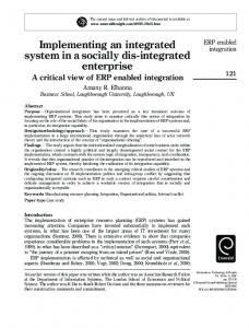
5% 10% 15% 20% E-commerce share of retail trade

Figure 1: B2C e-commerce sales share of retail trade in selected countries in 2015 (14)

E-Commerce The lately increasing utilization of internet technologies in retailing led to numerous new online retailers and marketplaces. It thereby also resulted in a transition of the entire business which mainly consists of business-to-customer (B2C) transactions. Nowadays e-commerce is well established and has a large stake in customer transactions in retailing. This trend is illustrated in Figure 1, considering the e-commerce shares of retail trade in selected countries in 2015, and Figure 2 depicts Germany as an example to show the evolution over the past years in more detail. Looking at the bar and line charts it is recorded that the total turnover as well as the share of retail trade is very high in countries like the United Kingdom, the United States and Germany and increased in the course of the years. This proofs the high importance of e-commerce in retailing. Additionally, Figure 2 shows the total e-commerce turnover in year 2015 divided into product groups. Here clothing and electronic products make up the largest shares. Clothing, shoes and other fashion products are particularly suited as applications of CLSC optimization models as a crucial fraction of ordered products are returned and these cause significant losses which the distributor have to bear (35). Another investigation in Germany conducted by the University of Bamberg and the “Bundesverband des Deutschen Versandhandels” (28) finds that the return rate for the product group clothing and shoes is, on average, 28.5 % and thus by far exceeds the second highest rate for electronic items which amounts to 15.6 %. At the lower end there are furniture items with a rate of 12.2 %. So clothing items not only make up the largest share of e-commerce turnover in Germany but also yield the highest return rate. The reasons for customers returning ordered products are wide-ranging like for example the size is not adequate or the product does not match customer’s expectations. But there is also opportunistic behaviour where customers misuse the possibility to return orders. However, this work does not go into further details on the reasoning for product

80

11.1% 11.1%

60 9.3% 8.2% 40

48.3

49.1

11.6%

12%

52.4

10%

39.3

8%

34 6% 4%

20

2% 0

2011

2012

2013 Year

2014

2015

0%

9

E-commerce turnover Share of retail trade

14% Share of retail trade

E-commerce turnover in EUR million


Product groups Clothing Electronic items Books & e-books Shoes Computers & software Furniture & decorations Household items Leisure items Films & music Flowers Others

Figure 2: B2C e-commerce turnover in Germany (2011 - 2015) (12), (13) returns and possible ways to influence and manage it. A good overview of this topic is given in (5). The decisive role of returns in e-commerce is also obvious when looking at customer satisfaction surveys. BearingPoint, a consultancy, finds in a study conducted in 2014 that customer satisfaction levels rank as most important indicator for the likelihood of purchasing articles via an online shop and these are influenced by the policies, namely the cost and conditions, for returning products (8). Therefore, a professional management of returns is needed in order to obtain a strong market position in the B2C e-commerce business. Lastly, an important characteristic of clothing products is a simple and cheap refurbishment process. For instance a returned garment is checked, if necessary, washed or ironed, packed and afterwards ready to be sold again to another customer. This process is also applied by most online retailers (28). Therefore, the CLSC in e-commerce retailing, where the return rate is high and returns can be refurbished easily, is a suitable example to apply the extended LIP. In addition to that, existing companies face a growing pressure for a high delivery service due to increasing customer expectations, which for instance also cover same-day-deliveries in urban areas. This fact urges retail companies to redesign their supply chain by applying a LIP. Lastly, there are quiet a few start-ups that need to design an entirely new supply chain and thereby face a greenfield scenario for which strategic location problems fit the best. Container Management Logistics assets and distribution equipment such as pallets, containers, tanks, bins etc. are of crucial importance in outbound logistics as well as

2

10


cross-plant deliveries. Outbound logistics activities relate to the last transportation leg, delivering finished goods to the final customers. Deliveries across different plants within a company are an element of intra-company logistics. Both are appropriate examples for set-ups in which the LIP with closed-loop and refurbishing considerations can be applied. However, the context differs from the prior example as the assets are mostly owned by the companies and, especially for intra-company logistics, the entire material flow is within the scope of the company. The motivation for companies to manage logistic assets follows cost calculations and the reasoning of green logistics. Green logistics extends the focus on cost-efficiency throughout all logistic activities within the supply chain, both outbound and cross-plant deliveries, by sustainability considerations and results in a growing prevalence of reusable equipment instead of e.g. disposable containers. Therefore, the integration of the reverse container flow into the forward flow rises in significance, too. There are some examples where reusable containers are traditionally widely spread like breweries or chemical and pharmaceutical companies. Breweries face a setting for crates and kegs which are delivered to customers, i.e. external parties, and returned to the company after usage. They have to bear substantial losses due to non-returned and damaged containers that have to be scrapped (11), although nowadays the utilization rate of glass package returns is generally estimated around 89% in Germany (27). Recycling glass received much attention on a macro-economic level at the end of the twentieth century which led to deposits on glass bottles what in turn resulted in rising return rates from 23% in 1980 to 79% in 1997 for Germany (25, p. 4). Another example with specific properties that also fits to the CLSC set-up are chemical companies. They mostly take on the collection and return process of their high-value assets, e.g. special tanks for hazardous liquids or gases. In addition, returned tanks need a more complex refurbishment process, comparing to crates and kegs. So altogether the reverse supply chain is of considerable importance for SCM departments in chemical companies. A particular characterisation of container management, comparing it to the prior ecommerce example, is broadly speaking a high return ratio. For instance in the case study of Alinovi et al. (1) a rate of 87% is assumed. However, it varies in terms of the economic value of the assets, i.e. high-value assets associate with a high return fraction. Moreover, the costs of refurbishment differ depending on the specific application, e.g. cleaning glass bottles or kegs is cheaper than refurbishing containers that carry hazardous chemicals. Health Care Next, health care services give a predestined application for integrated location-inventory models, as the location of facilities impacts the quality of the services. Additionally, the cost of failures or wrongdoing is very high, potentially a loss of life. For instance the research of Shen et al. (56) is motivated by work they did for a blood bank,


11

in particular looking at the production and distribution of platelets. Because platelets are highly perishable and need special treatment while storing, they are very expensive. Furthermore, the demand is highly variable. Another example is given in (37, p. 437). Herein the authors mention the design of a network for organ transportation which mostly shares the characteristics of the blood bank example. Both examples demand well-organized logistic operations and these are influenced by the location of facilities and the policy of inventory management. Three reasons are identified for that: First, delivering on time is very important and thus facilities need to be located in such a way that certain delivery time requirements are met. This is due to the fact that the service level, meaning for example less deaths, increases with respect to the proximity. Second, emergency deliveries, needed in case of stockouts, are expensive and increase the total transportation cost. So a network in which inventories are stored decentralized at many facilities is more desirable, as emergency delivery distances are minimized. Third, variations in demand cause high safety stock levels at all facilities. Therefore, the utilization of risk-pooling effects in inventory management needs to be considered in order to reduce total safety stock levels without lowering the target service level. All in all, an exceptional characteristic of health care applications is the predominant interdependency of location and inventory decisions and the integrated LIP in a closedloop set-up is able to address these trade-offs and to support decision making.

Service Parts Especially in the machine engineering industry and the automotive industry, service parts play a crucial role within SCM. Customers increasingly expect a high service level for the purchased products throughout the entire life-cycle. This implies for companies that the service part supply chain needs to be designed efficiently, which means offering a high product availability to any customer and for any product out of a potentially large product portfolio. Additionally, the demand is mostly stochastic as machines or respectively cars do not break down with a deterministic pattern. Therefore, an integrated LIP is highly suitable in the network design planning process for service parts, as the demand is stochastic, many product variants exist and a high service level is required. A high service level also requires fast deliveries, which are influenced by both the location and the inventory decisions.

All examples just mentioned have in common that applying the corresponding mathematical optimization problem, namely the LIP in a CLSC with product refurbishment, prospects significant cost-savings due to a more detailed and adequate modelling approach that covers various problem characteristics. Thereby it overcomes drawbacks that exist for traditional approaches that make too many over-simplified assumptions.

2

12


2.2

Fundamentals and Literature Review

Before presenting the integrated LIP in a CLSC with product refurbishment, a comprehensive literature review is given to outline the current state of research in this area. In addition to that, affiliated basics are mentioned that are used in the course of this work such as different problem types and solution methodologies. The sub-section concludes with the statement of the research contribution. 2.2.1

Classification and Distinction of Location and Inventory Problems

To begin with, an overview of alternative problem types for location and inventory problems is given. The intention is to introduce and categorize existing models and thereby also differentiate the approach used in the present work. 2.2.1.1 Location Problems The research on determining the number and location of facilities traditionally considers installation as well as transportation costs and the customer demand. With respect to these parameters some basic problem formulations are the Weber problem, dealing with only one facility in a continuous space, and the more general discrete Warehouse Location Problem (WLP), also known as Facility Location Problem (FLP) or the location-allocation problem. Extensions to these simple location problems allow capacities at facilities, different types of facilities, multiple products that flow through the network, extended supply chains in terms of the number of levels that are taken into consideration or dynamic models that modify the planning horizon and analyse more than one time period. Some comprehensive reviews are given in (18), (37), (38) and (46). In location theory, there are basically three different types in terms of the topography used: Planar, network and discrete models. The former case gives a set-up in which a facility can be located anywhere within a certain area like the Weber problem. Thus, the feasible area is assumed to be continuous what may turns out to be unrealistic in a real-world case, as in hardly any application an entirely greenfield situation is given. Next, network models are based on graphs containing a set of vertices and edges. Feasible locations are defined by either only the vertices or the set of vertices and along the edges. In such a model the distances are generally determined by the network what is a realistic model if the transportation infrastructure is restricted to a set of connections such as the rail network. Finally, discrete models extend the network model in so far that only a set of vertices is assumed and any transportation link between two vertices is allowed. Thereby the fixed set of edges is dropped. This type is used in the present work, as it is most suitable for a wide range of real-world applications in SCM, particularly the examples mentioned in Section 2.1. In general, a discrete location problem abstracts from a specific underlying distance


13

function and any mathematical metric can be applied to determine the distance between two vertices in a two-dimensional space. The most familiar distance function is the Eup clidean metric, defined as: d(x, y) = kx − yk2 = (x1 − y1 )2 + (x2 − y2 )2 . Especially when looking at distribution networks using lorries to transport goods, the distance function is refined by extending the straight-line Euclidean distance function to the straightline distance between two points x = (x1 , x2 ) and y = (y1 , y2 ) on the surface of a sphere, namely the great-circle distance given by the haversine formula: s y2 − x2 y 1 − x1 2 2 + cos(x1 ) · cos(y1 ) · sin c(x, y) = 2 · arcsin sin 2 2 d(x, y) = r · c(x, y)

[km]

where x1 and y1 are the latitude, x2 and y2 the longitude of the two points and r is the radius of the sphere, here the earth. 2.2.1.2 Inventory Problems Models for inventory management focus on the delivery reliability. In doing so, the determination of an ordering policy is targeted to ensure that enough supplies are available and commonly inventory holding costs are taken into account that compromise cost related to keeping and maintaining stock on hand in e.g. a warehouse. In addition to that, ordering costs apply as fixed charge for each order placed at a supplier. Together these result in a trade-off which is also known for the lot-sizing problem. The Economic Order Quantity (EOQ) formula computes the optimal order quantity in such a setting. The books (17), (45) and (66) give a comprehensive overview of inventory management. First and foremost inventory problems are distinguished in deterministic and stochastic types, depending on the input parameters. The former assumes that all parameters are known upfront and specified for the entire planning horizon. However, the customer demand, being the parameter with the greatest influence on inventory calculations, is mostly subjected to a high degree of uncertainty, representing the stochastic type. Here uncertainty is referring to a deviation of the actual demand from the expected demand. Note that because of that the research on inventory management also considers forecasting methodologies and focuses on the accuracy of these techniques in order to reduce deviations between forecast and actual values, especially for a long planning horizon. Stochastic inventory problems take the inherent uncertainty into consideration and thereby intuitively result in more appropriate models. The stochastic parameters are commonly specified with a continuous probability function, e.g. the normal distribution function, or a discrete probability function that states probabilities for a set of parameter values. Other than stochastic demand, three further parameters are commonly assumed to be subjected to uncertainties (48, p. 253): First, the quantity received from the supplier can vary due to partial, incorrect or defective deliveries. Second, the actual stock on-

2

14


hand may differ from the current system data which are available for planning. Lastly, fluctuations in delivery times are frequently incorporated into inventory management models, as these occur very often due to e.g. traffic jams. Apart from that also cost factors are subjected to uncertainty and thus influencing the output of decisions in inventory management. The present work focuses on stochastic demand and assumes a normal distribution with known mean and variance. The newsboy problem is a well-known mathematical problem which is, amongst others, applied in the domain of stochastic inventory planning. The initial set-up addresses the situation of a newspaper vendor who buys newspapers for a fixed price and sells them on the same day for a given price. In doing so, the vendor faces a stochastic demand and newspapers can only be sold on the same day, i.e. the considered product is perishable. In logistics this model serves as archetypical example and is extended to consider fixed ordering cost and inventory holding cost (59, p. 120). In addition to that, inventory problems are separated into static and dynamic problems. Dynamic problems address a finite planning horizon in which for instance the demand varies for different time periods and decisions are made in each period. Important applications of dynamic inventory problems are cases in which seasonal demand occurs, e.g. the retail business usually has a peak around Christmas. On the contrary, a static inventory problem makes decisions only once and basically assumes an infinite planning horizon.

Going into more details on ordering policies and safety stock considerations that are commonly used in inventory management, the remainder of this paragraph describes some fundamental assumptions and calculations. An ordering policy determines two aspects of inventory management: When to place an order, i.e. the timing of an order, and how much to order, i.e. the order size. These decisions are subjected to cost parameters as stated above and the objective is to achieve a high product availability to be able to satisfy customers’ demand. Furthermore, these two aspects result in two dimension to characterise ordering policies: On the one hand, the review period and, on the other hand, the order quantity. The former can be either a specific period T or a continuous review, where a so-called Re-Order Point r (ROP) is defined, continuously monitored and orders are placed when the inventory level falls below the ROP. For the latter it is possible to determine a fixed order quantity Q or to allow variable quantities and always order up to a certain stock level S. An overview of all feasible combinations is given in Table 2. Note that the combination of a fixed order quantity and a fixed review period does not have any variable scope for decision making and thus it is not of relevance in practice (4).


15

Inventory level Replenishment time

Replenishment time

Q ROP r

Place first order

Place second order

Safety stock t1

t2

Time

Figure 3: Inventory management – (r, Q) model with safety stock considerations

Review period

fixed variable

Order fixed − (r, Q)

quantity variable (T, S) (r, S)

Table 2: Feasible ordering policies in inventory management In the following, the common (r, Q) is considered which is suitable for a strategic decision level (45). The general concept of the (r, Q) policy is illustrated in Figure 3. The chart displays the inventory level over the time and is exemplary limited to two ordering processes. The first order is placed when the inventory level reaches the ROP r at t1 and after the replenishment time the ordered quantity Q arrives and the amount is added to the inventory. The influence of variations in demand is shown in case of the second order process and described in the next passage. If the demand is not deterministic and varies between time periods, the cumulated demand during the replenishment time possibly exceeds the stock on-hand. There are basically two different approaches to incorporate the influence of stochastic parameters into the model. On the one hand, a target service level can be defined a priori and consequently not all orders are satisfied. On the other hand, a shortage cost parameter can be introduced which means there is a trade-off within the decision making process between shortage cost and the other cost parameters, e.g. ordering and holding cost. Consequently, in the optimal solution only a certain amount of shortage cost is tolerated. In the following the first approach is used, as in practice it is quite difficult to quantify shortage costs and currently most companies have service level definitions in place (17). The service level approach takes all stochastic parameters that are relevant to the decisions, meaning all deviations from the average case, into account. There are various service level definitions

2

16


which also consider different types of application. The most common are the following two (4): 1. Type I (α service level): Probability that, within a given period, all orders are satisfied instantly and in full. Note that this definition equals to the number of events when there are no stockouts. 2. Type II (β service level): Proportion of the total demand, within a given period, which is supplied instantly. Note that this definition is equivalent to the weighted number of events when there are no stockouts, whereas the weights are given by the amount of demand. Hereafter the Type I service level definition is used. In order to further elaborate the properties of the Type I definition when applying it in the context of the (r, Q) ordering policy, the following underlying mathematical model is considered, which describes the ordering process: Q µ min o · + h · r − µl + Q 2 s.t. P(L ≤ r) ≥ α r, Q ≥ 0 Here ordering cost o and holding cost h are considered that add up to the total cost in the objective function. The normally distributed random variable L with mean µl represents the demand during the replenishment time and µ equals the demand rate. The probability of no stockouts is given by P(L ≤ r) and depends on the ROP r. In summary, this mathematical model minimizes the total cost by varying the ROP r and the order quantity Q such that a certain threshold α for the probability of no stockouts is guaranteed. As the decision variables r and Q are independent, they can be separated. Hence, the optimal order quantity is determined by applying the first-order condition on the term: o · Qµ + h · Q2 . The result is the well-known EOQ formula: Q=

r

2·o·µ h

(EOQ)

In order to further specify the probability P(L ≤ r) and thus determine the ROP r, one takes a second look at the chart of Figure 3. Note that for the first order the demand during the replenishment time is less than expected, as the inventory level does not touch the safety stock level. The second reorder process shows this fact more precisely. Each line, either solid or dashed, indicates a possible trend for the inventory level during the replenishment time after the inventory level reaches the ROP and an order is placed. The


17

slope of a line corresponds to one possible occurrence of the random variable L. The mean demand during the replenishment time µl is indicated by the solid line and one can see that it hits the safety stock level at the end of the replenishment time. Because the demand is assumed to be normally distributed and independent between consecutive periods, these lines are summarized in a density function which again turns out to be normally distributed with mean l · µ and variance l · σ 2 . Thus, the random variable L is defined by: L ∈ N (l · µ, l · σ 2 ). The density function is illustrated by the rotated Gauss curve and the mean is equivalent to the safety stock level. So the probability that there is a deviation, either positive or negative, between the actual inventory level after the replenishment time and the safety stock level follows the normal distribution. Furthermore, this implies that the probability P(L ≤ r) is given by the integral of the density function where the inventory level is above zero. The so called safety factor that guarantees a certain probability α for no stockouts is given by the inverse of the standard normal cumulative distribution zα = Φ−1 0,1 (α). This again can be translated into the safety stock needed by the following formula: √ S = zα · l · σ 2 So the ROP r is calculated by summarizing the safety stock S that is needed to compensate variations during the replenishment time and the mean demand during the replenishment time µl = l · µ: √ r = l · µ + zα · l · σ 2 In conclusion, the aim of this work is to use a discrete location model to describe the aspects that refer to the facility locations within the close-loop supply chain and the underlying inventory problem is modelled with stochastic input parameters. The inventory problem applies the continuous normal distribution probability function to describe the stochastic nature of the demand and the planning horizon is infinite. Thus, the model as such assumes a static steady state which also reflects the desired strategic nature. 2.2.2

Review of the Location-Inventory Problem Literature

The LIP is based on two streams of research: On the one hand, the location problem, i.e. the design of a network of facilities, and, on the other hand, problems in inventory management, i.e. the determination of inventory levels across a given network of facilities. The research on each stream alone is exhaustive and a rich literature is available, as already mentioned in Section 2.2.1. Melo et al. (38) identify a lack of simultaneous supply chain planning, in particular the integration of tactical and operational decisions into the strategic location decision. Daskin (18) also presents the integrated LIP as extension of classical location models. Hereafter a review on the evolution of research related to the

2

18


DCs Production site S1

Retailers µ1 , σ12 µ2 , σ22 µ3 , σ32 µ4 , σ42

S2

µ5 , σ52

Figure 4: Supply chain illustration for the risk-pooling effect integrated LIP is outlined and the major findings up to now are summarized. A general survey on integrated supply chain design problem, including LRPs and Inventory-Routing Problems (IRP), is given in (55). In the domain of integrated LIPs one trade-off prevails that has a significant impact on the solution, namely the risk-pooling effect. Prior to the introduction of the LIP, first studies on the effect go back to Eppen in 1979 (21) who investigated the cost saving potentials of centralization for a multi-location newsboy problem. The risk-pooling effect results from a concave non-linear square root term in the safety stock formula (S = √ l · σ 2 ). An illustrative supply chain example is given in Figure 4. The threeΦ−1 0,1 (α) · level set-up includes one production site, two DCs, five retailers with mean demand µi and variance σi2 and a feasible allocation of retailers to DCs is stated. For now other parameters and decision variables are neglect. The safety stock Si at each DC is proportional to p the square root of the sum of the variances assigned to it, i.e. S1 ∼ σ12 + σ22 and p S2 ∼ σ32 + σ42 + σ52 . If one decides to locate only one DC and to allocate all retailers to p it, the total safety stock level would be proportional to σ12 + σ22 + σ32 + σ42 + σ52 what is obviously less than S1 + S2 . This trade-off is called risk-pooling effect, as the risk, i.e. the total demand variance, is pooled at fewer facilities. The effect results in significant cost savings, if holding costs are high comparing to other cost parameters or the fluctuations in demand are considerably high (40). Finally, note that for now a normal distribution was assumed and any correlation has been neglect, although the size of the risk-pooling effect, meaning the difference of inventory levels and respectively total costs, also depends on the correlation of demand at the retailers and is either influenced positively or negatively. Schmitt, Sun, Snyder and Shen (53) investigate the optimal design of multi-location supply chains that are subjected to disruptions and uncertainties. They support the statement that in the absence of deterministic predictable demand the risk-pooling effect favours a centralized supply chain design, whereas supply uncertainties foster a decentralized set-up. The computational results of the present work fit to these results and a


19

decentralization trend is found. Chronologically the first studies on the LIP as such were conducted around the turn of the millennium. Erlebacher and Meller (22) were among the first who formulated an integrated LIP that takes location, transportation, holding and ordering cost for a twolevel supply chain into account. They use a unit-square grid structure to formulate the problem and demand is distributed uniformly across each grid. Due to the high complexity of the resulting problem, including non-linear terms, they use a heuristic algorithm to solve it. They also determine boundaries for the total number of facilities based on a relaxation approach. Additionally, Nozick and Turnquist (47) formulate a so-called fixed-charge facility location model, considering fixed costs and transportation costs, and extend it to take inventory costs and safety stock into account. For this purpose they perform a regression analysis and approximate the safety stock, and thereby the inventory cost, for a given number of facilities. The linear function is integrated into the fixed-charge location model and results are obtained by implementing a heuristic solution algorithm. The heuristic algorithms described and implemented in course of the present work partially follows the basic approaches and heuristic strategies stated in both publications, (22) and (47). A more generalized location-inventory model is presented subsequently by Daskin, Coullard and Shen in (19) and (56). Both study the same model but each presents a different solution approach. The former solves the non-linear integer problem by implementing a Lagrangian relaxation algorithm, whereas the latter uses a set partitioning solution approach. Motivated by the importance of inventory management in the B2C e-commerce business, a three-level supply chain with suppliers, DCs and retailers is presented. The demand is assumed to be a normally distributed random variable with given mean and variance and a safety stock at each DC ensures that a certain service level is met. Comparing both solution approaches for consistent datasets with 49, 88 and 150 nodes, the authors find that the Lagrangian relaxation algorithm is favourable in terms of computation time, but similar in terms of the solution quality. The datasets Daskin et al. proposed in their work to test their solution approaches have been widely recognized and used in many following publications as benchmark datasets. One assumption which is made in (19) and (56) on the mean and variance of the normally distributed demand prevents some artificial outcomes that are non-intuitive and hardly any SCM decision maker would take such a decision in reality. They assume the same variance to mean rate for the demand of all retailers and proof that thereby theses cases are excluded. One artificial outcome they deal with is that a retailer is not assigned to the closest DC. This is due to the risk-pooling effect that arises from concave non-linear terms in the presence of safety stock considerations. The authors design the

2

20


A

B

C

fA = M µA = M σA2 = 0

fB = 0 µB = 50 σB2 = 5

fC = 0 µC = M σC2 = 5

Allocation:

Location selected:

Figure 5: Exemplary non-closest retailer-DC assignment example depicted in Figure 5 to illustrate these outcomes. The set of feasible DC locations is equivalent to the retailers and given by {A, B, C} and the location cost fi , the mean µi and the variance σi2 of demand at each retailer are stated below in Figure 5. Without loss of generality, transportation cost between A and B as well as B and C are defined as constants. As M > 0 is an arbitrary large number, no DC is located at A, however B or C are both feasible, as location cost are zero. Next, it is cheaper to deliver from B to A than from C to A and thus a facility is definitely located at B and B supplies demand µA with no variance in the optimal solution. Finally, B and C both have the same positive variance σB2 = σC2 > 0 what allows benefits due to risk-pooling p p p effects, if they are delivered from the same location due to: σB2 + σC2 > σB2 + σC2 . Moreover, demand at C is very high and thus it is optimal to locate another facility at C and C supplies the demand of B and itself. So in this example not only a non-closest retailer-DC assignment occurs but also the demand of one location is assigned to another DC although a DC is located at the particular location. The mathematical formulation and conventions used in this work are based on the model of Daskin et al. However, the assumption related to the mean to variance ratio is not added, as examples like the one of Figure 5 are explicitly investigated in the computational experiments in order to see if they happen in practice. Miranda and Garrido enhance the LIP in (40) and (41) as formulated by Daskin et al. to also incorporate capacity constraints for any opened DC. They present a Lagrangian relaxation algorithm which is also based on the sub-gradient method. Furthermore, in (40) the authors obtain computational results by applying it to a dataset with 10 feasible DC locations, 20 customers and varying parameter settings. Thereby they recommend that the integrated model should be applied, if the products considered are perishable, i.e. inventory cost are high, or of high value as cost savings exist in comparison to a sequential approach. In (41) they choose a slightly larger dataset consisting of 20 feasible DC locations and 40 customers. Here the results lead to the insight that tighter capacity constraints do not always call for an increase in the number of DCs, just like an increase in demand variance at retailers. So the results of both studies are somehow contradictory


21

and it can be noted that the findings are highly dependent on the dataset and parameters which are used. In addition, a validation with real-world data is essential. They continue their research on LIPs in (42) and present a model in which the service level is not predetermined, but a decision variable on its own and thus determined in the course of the optimization. This is achieved by introducing an extra cost parameter, namely penalty costs for unfulfilled demand. However, penalty costs are hard to specify in real-world applications and they also increase the computational effort and the complexity of the problem. Therefore, the authors design a simplified iterative and sequential twophase algorithm in which an initial service level is set, subsequently the LIP is solved for the fixed service level value and finally the value is updated, if needed. Note that the penalty costs function decreases with respect to the service level, whereas the function of all other cost parameters, which they call operating cost, increases. Thus, an equilibrium exists, if there is no incentive to deviate from a certain service level and the authors are able to formulate the equilibrium condition. If the described algorithm reaches the equilibrium, it terminates. A similar safety factor analysis to (42) is performed in Section 3. Furthermore, the capacity restrictions are taken from these publications and the insights on the question, when to apply the integrated model, are considered. Snyder, Daskin and Teo (61) extend the literature on LIPs by presenting a stochastic program that is subjected to uncertain parameters which are summarized to discrete scenarios. In doing so, they formulate a model that minimizes the total expected cost across all scenarios and describe a Lagrangian relaxation algorithm which they use to solve problems with up to 150 nodes and nine scenarios. They define parameters that are scenario-dependent, e.g. demand means and variances or transportation costs. Moreover, some decision variables are scenario-independent, e.g. where to locate a DC, and others are scenario-dependent, e.g. how to allocate retailers to DCs. Note that each scenario determines the demand mean and variance at retailers, which are still stochastic parameters. Computational results are drawn from the datasets provided by (19) and (56). Comparing the solution obtained by the stochastic model with the optimal solution for each scenario they find a roughly 8% regret on average and nearly 25% regret in the worst case. The regret value is defined in terms of the objective value of the best stochastic solution found comparing to the optimal solution for a single scenario. Moreover, they confirm the hypothesis that a single scenario solution falls behind the stochastic solution in the long-run. Chen, Li and Ouyang (15) investigate the robustness of LIPs in the presence of facility disruptions, e.g. caused by natural disasters. They propose a non-linear Mixed-Integer Program (MIP), including facility failures with a given probability, and apply a Lagrangian relaxation algorithm to get some managerial insights. The set-up of the so-called reliable

2

22


facility location design framework assumes that after the breakdown of a facility all customers assigned to this facility are reallocated to other existing facilities. They find that the number of located facilities increases and the locations tend to accumulate in clusters when the failure probability increases. Obviously, also the total cost increase comparing to the simple LIP. The results are backed by the findings of Schmitt et al. (53), concerning risk-pooling, risk-diversification and supply chain disruptions. A similar approach to (61) is implemented in this work to analyse the solution obtained for the LIP in a CLSC with product refurbishment in the presence of risk and the following definition for uncertainties, introduced amongst others by Snyder in (60), is considered: Definition 1. In a risk environment, probabilities are known for the uncertain parameters and a stochastic program is used to determine the risk-optimal solution that minimizes the expected total cost. On the contrary, an environment where no information is available for the uncertain parameters is actually called uncertain and associated to the domain of robust optimization.

The concave non-linear inventory terms to determine the order quantity as well as the safety stock and the complexity of the simultaneous location and allocation decisions make the LIP difficult to solve to optimality. A common approach to resolve non-linear terms is a piecewise-linearisation. Vidyarthi et al. (64) presented such a linearisation for a nonlinear MIP, namely an integrated production-location-inventory problem with multiple products. They conclude that the piecewise-linearisation gives a good approximation and their Lagrangian relaxation solution is within 5% of the optimal solution. The same linearisation approach is applied in the present work. Another capacitated version of the LIP is presented by Ozsen, Coullard and Daskin (49) and named capacitated warehouse location model with risk-pooling in order to emphasize the importance of the risk-pooling effect. The stock level is computed as the sum of working inventory and safety stock and the worst-case is assumed to stipulate that capacities are met at any time. The authors note that capacities, in this sense, allow the evaluation of the trade-off between the following three alternatives: Open additional facilities, reallocate customers’ demand or reduce the order quantity and thereby lower the circulating stock. They obtain computational result by applying a Lagrangian relaxation algorithm to the datasets presented by Daskin et al. in (19). Another extension, namely the possibility for any retailer to use multiple sources, DCs respectively, is investigated in a following research by the same authors in (50). They find in both studies that for increasing transportation costs the number of DCs opened is higher and more retailers utilize the multi-sourcing option. The former is also underpinned by computational results in the present work.


23

Atamt¨ urk, Berenguer and Shen (6) extend the model of Daskin et al. in various ways. Their research is motivated by the application of a “new” modelling approach, namely conic MIP or SOCP, which is explained on page 24. Conic MIPs allow a more general modelling approach and the models become more realistic. Moreover, they are solved efficiently with standard solvers. The authors start with the basic uncapacitated LIP from (19) and (56) and subsequently add: Capacity constraints for the DCs, multiple commodities and another stochastic parameter, namely stochastic replenishment times at DCs. Furthermore, the independent normal distributions for retailers’ demand are let to be multi-normal distributed random variables with given means and variance-covariance matrices. Thereby the formulas, in particular the safety stock formula, are generalized to allow correlated demand. The present work takes on the SOCP modelling approach because the application of standard solvers is much more convenient. It provides a major advantage comparing to other solution approaches mentioned up to now, as for instance Lagrangian relaxation and column generation approaches require either highly specialized algorithms or extensive programming effort (6). Furthermore, numerical experiments reveal that the conic formulation outperforms the Lagrangian relaxation in (56) and (49) with respect to the computation time.

A comprehensive review on the LIP is given in (23). The authors present a basic formulation of the LIP model as well as an extended LIP model that combines vehicle routing, inventory management and location planning. Furthermore, they show various classifications of publications with respect to solution techniques, model attributes, cost components and case studies performed in the domain of LIPs. Finally, they identify some directions for future research.

2.2.3

Closed-Loop Supply Chain Literature

The research on CLSC is growing, as decision makers in SCM demand models that reasonably describe the supply chain they are managing and trying to improve. As aforementioned, the latest SCOR framework version also recognizes “return” as one key management process. Furthermore, for reasons of sustainability, the legal environment as well as cost-efficiency assessments put the spotlight on CLSC. Because the literature in this domain is versatile, the section shall first categorize and clearly distinct some fundamental terms that are used in this work and then the relevant publications are outlined.

2

24


Second-order cone programming (SOCP): The domain of convex, non-linear quadratic optimization problems can be divided into two separate sets of optimization problems: Firstly, the objective function can be a convex quadratic function while the constraints are linear. These problems belong to the set of Quadratic Programs (QP). Secondly, the objective function can be linear but the constraints contain convex quadratic terms (Quadratically Constrained Program, QCP). If both are given, the program is named Quadratically Constrained Quadratic Program (QCQP). The SOCP is a special case of QCPs and has the following general form (6): min f T x s.t.

kAi x + bi k2 ≤ cTi x + di

i = 1, · · · , p

where the variables and parameters are defined as: x ∈ Rn , f ∈ Rn , Ai ∈ Rmi ,n , bi ∈ Rmi , ci ∈ Rn , di ∈ R and k·k2 is the Euclidean norm. Note that for Ai = bi = 0 the problem can be transformed into a linear program and by letting cTi = 0 it reduces to a convex QCP. Furthermore, by adding additional variables and constraints the objective function of a convex QCQP can be linearised and thereby translated into an equivalent SCOP (2). An illustration of a simple second-order cone restriction kx1 + x2 k2 ≤ x3 which is p equivalent to x21 + x22 ≤ x3 is depicted in Figure 6. Obviously, a SOCP is always convex, as the second-order cones are convex sets. The convexity-property of SOCPs allows the application of efficient solution methods. One example are interior-point algorithms that are able to solve SOCPs efficiently and have been developed further in the recent years (6). Due to this fact and a wide range of applications, SOCPs received an increasing focus. Now for example CPLEX is able to detect and solve SOCPs, respectively MIQCPs, by applying a branch-and-cut based solution approach. x3

x2

x1

Figure 6: Exemplary convex second-order cone: kx1 + x2 k2 ≤ x3


25

2.2.3.1 Distinction of Closed-Loop Supply Chain Definitions There are two streams of research that equally lead to CLSC. On the one hand, an increasing focus on the importance of environmental issues and sustainability of logistic operations drive the advancement of the field around green logistics, named hereafter as first stream. Green logistics aims to reduce the ecological impact and thus reusing returns is one important approach to achieve this objective. Srivastava (62) presents a comprehensive conceptual framework and a network configuration for green logistics. The classification used in his study assigns the reusage of returned products to green operations in logistics, which in turn cover, amongst others, refurbishment of returns what is considered in the present work. Another affiliated area that touches CLSC and also belongs to green logistics is the management of returns. According to Asdecker (5, p. 23) management of returns extends the scope and takes operations such as the prevention of returns or efficient processing of returns into account. However, this aspect is not scrutinised in this work. On the other hand, the term supply chain initially only refers to the forward flow of products, starting at the raw materials and ending at the customers. In this context, reverse supply chain starts at the end-customer and considers “the process of planning, implementing, and controlling the efficient, cost effective flow of raw materials, in-process inventory, finished goods and related information from the point of consumption to the point of origin for the purpose of recapturing value or proper disposal.” (52, p. 2) Therefore, the second stream of research, regarding reverse supply chain in its technical sense, equally leads to the consideration of the CLSC set-up in which the reverse supply chain is integrated into the forward supply chain. Thus, the objective of the second stream of research is to rather focus on the economic benefit of the possibility to reuse product returns whereas the first stream is motivated by sustainability targets. Reasons why customers return products are manifold and this work focuses on those mentioned in Section 2.1. A classification of the flow of materials and the operations that are present in a CLSC are illustrated in Figure 7 which is derived from (62). The illustration is based on a four-level supply chain and returned products are first checked and afterwards either disassembled or refurbished. Disassembled units face three options: Remanufacturing, recycling or scrapping. Note that these operations do not have to be performed at different facilities. The figure also defines some basic terms used in the following. For instance refurbishment and remanufacturing are differentiated with regard to the point, where the end-products are reintegrated into the forward supply chain. The former are directly reused in the DC as only minor repair operations are needed and the latter processes units that need, at least partly, disassembly and are reused in the aftermath at the production site. In conclusion, the CLSC approach of this work takes only refurbishment and the scrapping-option into account which are grey-highlighted in Figure 7. Furthermore, it

2

26


Raw Material

Production Site

Distribution Centre

Customer

Recycle

Remanufacture

Refurbish

Check Disassemble Scrap

Focus of this work Figure 7: Material flow and operations in a CLSC explicitly addresses the integration of the product flows and not merely extends the supply chain to cover more levels, e.g. disposal centres. The following precise definition is used that is affiliated to (29): Definition 2. Decision makers in a Closed-Loop Supply Chain (CLSC) aim to capture additional value by integrating activities that consider the collection of returns from the end-customer, reverse transportation, checking, deciding whether to reuse or dispose and finally performing the selected option, what may include redistribution. 2.2.3.2 Closed-Loop Supply Chain Literature Even though there are at present hardly any publications studying integrated LIP in a CLSC, the remainder of the section outlines publications that are affiliated to it and some analytical models as well as solution algorithms are presented. Diabat, Abdallah and Henschel (20) based their research on the LIP, how it has been introduced by Daskin et al. in (19) and (56), and apply it on a CLSC that considers spare parts. Their motivation follows the high share of product life cycle costs (up to 85%) that are influenced by supply chain decisions. The three-level set-up goes as follows: The forward supply chain satisfies stochastic demand at retailers for a single product. The reverse supply chain collects returned products in so-called remanufacturing centres, where those are remanufactured as spare parts and subsequently delivered to the retailers. Depending on the constant variance-to-mean ratio for each retailer, they present a Lagrangian relaxation algorithm to solve the non-linear MIP as previously proposed by Daskin et al (19). Note that no capacities are considered and that the closed-loop integration, meaning the re-entering of returns into the forward flow, comes just with a single constraint that ensures that remanufacturing centres are co-located with DCs and thereby the same retailers that are allocated to a DC are also supplied with remanufactured units from this location. The authors find that for high inventory cost the number of facilities decreases whereas more facilities are used if the transportation cost are high. Additionally, the


27

transportation cost have a huge impact on the time needed to solve the problem. The aim of this work is to examine these computational result. Furthermore, the authors point out extensions as for example capacity constraints or assuming that returned products can be refurbished to as-good-as-new products and reused in the forwardoriented supply chain. Both extensions are covered in the present work. Another integrated CLSC model for inkjet cartridges in Hong Kong is proposed by Chen, Chan and Chung (16). They formulate a MIP that takes location and allocation decisions, capacities at all relevant facilities and the decision whether to recycle returned units or not into account. In addition, returned units are considered to be of different quality levels. However, they miss out stochastic demand and thus any non-linear terms resulting from safety stock calculations. As the model is intractable for real-world instances, they present a genetic algorithm to obtain results. They find that the algorithm is competitive and achieves near-optimal solutions in less computational time. Zhang, Berenguer and Shen (65) extend the research conducted by Atamt¨ urk, Berenguer and Shen (6) and present a capacitated facility location model for a three-level supply chain with bidirectional flow of materials. In doing so, they address an increasing attention in operations management of returns and call their network a CLSC. The forward flow of materials is identical to the study of (6). The reverse flow starts at the retailers and is then directed via corresponding DCs to the suppliers. As the only interaction of the forward and reverse flow of products is given by savings from co-locating forward and reverse DCs at the same location and no reusage of returns is considered, their definition of CLSC differs from Definition 2 used in the present work. Analogous to (6), Zhang et al. reformulate the non-linear MIP in order to employ a conic integer programming approach. The present work further extends the bidirectional flow model and integrates the reverse flow into the forward flow of products. More recently, Kaya and Urek (32) examine a non-linear MIP for a CLSC network design problem that integrates location, inventory and pricing decisions. Thus, the objective is to maximize the profit what distinguishes it from all other studies mentioned up to now. The CLSC composes the separated distribution and collection of products via a network of so-called collection and distribution centres (CDC). As the model is highly non-linear, what is also due to the pricing decision that considers retailers’ price sensitivity of demand, they propose a heuristic solution approach which utilizes a piecewise-linearisation for the concave square root function and three metaheuristic algorithms, namely: Simulated annealing, tabu search and genetic algorithm. They find that heuristics perform well in trials where they compare it with the optimal solution for 10 customers, though they analysed datasets with up to 200 customers. On average the tabu search heuristic outperforms the other two heuristics in terms of solution quality.

2

28


Remark on Inventory Problems in a Closed-Loop Supply Chain: This subsection on the current state of research on the CLSC closes with a brief remark on inventory management. As aforementioned, models for inventory management are extensively available. Schrady (54) was amongst the first who investigated the reusage of returns in 1967 for a deterministic inventory model. He basically presented an EOQ-like formula for the net-demand, meaning total demand less the number of returns on-hand. More recently Mitra (43) analyses a two-echelon inventory system for a closed-loop setting and proposes a deterministic and stochastic model. The former is similar to the one suggested prior in (54) and the author mentions that it corresponds to a basic dual-supplier inventory problem. Multi-supplier models have the characteristic that a company can decide which supplier(s) to choose and how much to order from each of them. This decision takes for instance the available capacity, the price, the replenishment time or the quality of delivery service into account. For the stochastic model, Mitra notes that this is very difficult to formulate for multiple echelons and some simplifying assumptions are needed e.g. normally distributed demand and returns, independence of demand and returns, high variation coefficients for all random variables and further assumptions to resolve convolutions of two random variables. The present work also covers a stochastic multi-supplier inventory model and makes similar simplified assumptions as explained in Section 2.3. Regarding the analogy of the CLSC with a multi-supplier problem, one difference stands out, namely the fact that in a CLSC returns are within the scope of the decision maker. Therefore, the decision maker can further improve the performance by reusing returns where it is cost-optimal to do so. This leads to a system that is similar to a set-up with lateral transshipment. Here this work only points out the analogy of both types of inventory models and summarizes the advantages of lateral transshipment by referring to the findings of a simulation study performed by Tagaras in (63). The author is looking at the effects of risk-pooling on an inventory distribution network with lateral transshipment. Thereby he finds that the service level, being the predominant performance evaluation criterion, is increased substantially without additional cost when transshipment is allowed. In other words, collaboration in terms of transshipment reduces the occurrence of stockouts and costly emergency deliveries. The insights are used in the line of reasoning of this work, as refurbished units can be transshipped to any DC within the network and thus a transshipment-like set-up exists. 2.2.4

Research Contribution

The goal of this work is to extend the research on LIP in a CLSC, where the term CLSC is defined as stated in Definition 2. The main contributions are outlined as follows: • First, a novel non-linear MIP is formulated for the LIP in a three-level CLSC with product refurbishment. The model covers location, transportation, inventory hold-


29

ing, ordering, refurbishment and scrapping costs as well as multiple products and all facilities have limited capacities. Thus, location planning addresses the facilities that are needed to design the distribution network and the inventory management at DCs integrates refurbished returns as a kind of second supplier. Altogether stochastic demand and risk-pooling effects are considered in the model. • Second, a conic MIP approach is employed as modelling technique to be able to apply standard solvers. Therefore, a reformulation of the non-linear MIP is presented to meet the requirements of a conic program. Additionally, a two-phase heuristic algorithm is proposed, which is capable of solving large instances. • Finally, computational results are studied that include new insights for decision makers in SCM. For instance an investigation analyses the saving potentials of an integrated LIP in the context of a CLSC comparing to the traditional sequential approach. Furthermore, an inquiry on the structure of the exact solution is carried out that promises insights for practitioners. Finally, a scenario analysis yields new findings on parameters that have a major influence on the solution quality as well as the structure and a risk-optimal solution is determined.

2.3

Formulation of the Mathematical Program

After giving a comprehensive overview of the latest findings in the academic literature and classifying the subject of this work, this sub-section proposes a mathematical model for the integrated LIP in a CLSC. First, some model properties are stated that rank, amongst others, as assumptions that are relevant to this work and define the application of the proposed mathematical model. Second, the decision variables, parameters and constraints for the model under consideration are put together into a non-linear MIP. Additionally, the different terms and trade-offs that compose the objective function are described. Lastly, a reformulation is used to transform the non-linear terms into a MixedInteger Quadratically Constrained Program (MIQCP). 2.3.1

Categorization of the Model Properties

There are various model properties that explain the characteristics of a location and inventory problem in SCM as already mentioned in the previous Section 2.2.1. Some that also extend these and altogether describe the considered LIP are listed hereinafter: • Multi-level supply chain set-up: The elements included in the scope of the LIP are production sites, DCs and retailers. These are arranged hierarchically, i.e. units are always transported from one level to the following. The CLSC set-up expands the forward chain to include returned products. The reverse chain is also arranged

2

30


hierarchically and consists of retailers, refurbishment centres (RC) and DCs, where the reverse flow is reintegrated into the forward flow. • Discrete set of feasible DC and RC locations: The set of all retailers equals the set of feasible DC locations as well as the set of feasible RC locations. So there is basically only one set of locations and the sets are not disjoint. Furthermore, no limitations on the allowable number of facilities exist. • Capacitated DCs and RCs: At each feasible DC or RC location the total number of units stored is capacitated. Furthermore, different sizes are defined which vary in terms of the maximum capacity. A stepwise function translates the type of DC or RC into cost values, respecting cost savings due to economies of scales. A minimum load for any opened facility is not assumed. • Un-capacitated transportation and production capacities: In contrast to the location capacities, transportation and production capacities are not limited and assumed to be available at any time and in any quantity. • Direct deliveries: No aggregation of deliveries is executed, i.e. vehicle routing decisions are not included and transportation cost are based on the number of units. Direct deliveries can also be recognized as customer visits at retailer sites where they individually purchase products or services. • Multiple products: Each production site operates as the sole producer and supplier for one kind of product. Thus, the number of products determines the number of production sites in the model. By and large the CLSC network design is productspecific and the mathematical formulation separate each product except for total inventory calculations at DCs or RCs. • Reverse logistics: Returned products are collected at RCs and then either refurbished, transshipped to a DC and reused to satisfy retailers’ demand, i.e. the as-good-as-new assumption holds true, or, if this alternative is to expensive, scrapping is taken into account. Scrapping is performed at the RC. • Static planning: The model horizon is limited to one period and thus the planning is static and decisions are made once at the beginning of the period. Likewise, the planning horizon is regarded as infinite and a steady-state is assumed. • Stochastic attributes: 2 – Stochastic demand D ∈ N (µD , σD )

– Stochastic returns R ∈ N (µR , σR2 )


31

The demand as well as the number of returned units at a retailer are normally distributed with mean µ and variance σ 2 . The random variables are mutually independent and thus the statistical correlation is zero and does not have to be considered when summarizing or splitting random variables. • Following decision-relevant cost parameters are considered: – Locating cost (per DC) – Transportation cost (per unit) – Inventory holding cost (per unit and time unit) – Ordering cost (per order) – Refurbishment cost (per unit) – Scrapping cost (per unit) In addition to this classification, there are some further assumptions that have to be considered before looking at the mathematical formulation of the problem in more details. It is assumed, as explained later in this chapter, that the total mean demand is supplied and the possibility to decide, not to consider a retailer at all, since it might be unprofitable for the company to do so, is not given. Furthermore, Axsater (7) indicates that using the deterministic EOQ formula for the (r, Q) ordering policy in the presence of stochastic demand, and first calculating the order quantity Q based on the mean values and then determine with Q the ROP r, is only a heuristic solution. However, numerical experiments yield that the performance of the heuristic approach is sufficient in practice and much better than theoretical worst-case bounds (56). 2.3.2

Relevant Decisions and Trade-Offs

Based on these assumptions the LIP in a CLSC considers the configuration of a distribution network to deliver goods from various production sites through a set of DCs to the retailers and thereby the demand is satisfied. The demand only occurs at a given set of retailer sites, which are spread over an area, and the production sites are also a priori known and fixed. Conversely, returned products are collected and refurbished at RCs and transshipped to DCs where they are reused to satisfy customers’ demand what is also in the scope of the LIP. Transshipment is herein defined as the transportation activities and other operations regarding the flow of goods from RC to DC sites. Figure 8 illustrates the three-level CLSC. There are various decisions that are composed in the present problem and these are described first in the following. The decisions are also reflected in the objective function and it serves as performance measure. However, the decisions are highly interdependent and in order to determine the optimal solution a simultaneous approach considers these

2

32


Production sites

Retailers DCs

RCs reverse

forward

Figure 8: Illustration of the three-level CLSC Index

Description

i j, j 0 k, k 0 p

Index Index Index Index

for for for for

retailers; I set of retailers DCs and RCs; J set of feasible DC and RC locations different facility types for DCs and RCs; K set of types different types of products; P set of products Table 3: List of indices

all at once. Note that the following elaboration is done sequentially and parameters and variables are gradually listed for the sake of clarity. A comprehensive list of all variables, parameters and notations is stated in Table 15 and 16 in the appendix. Finally, Table 3 summarizes the four types of indices used in this elaboration. 1. DC location: Out of the given set of feasible DC locations, only a few are selected, as opening a facility at a location induces costs. These costs are fixed and reflect e.g. expenses for building a new DC. Due to the fact that the size of a DC, defined in terms of storage units or storage and retrieval operations, can vary a lot and has at the same time a huge impact on the occurring costs, different DC types k are considered. This is represented by a stepwise constant function and implemented as cost parameter fj,k for a DC facility of type k at location j. The related binary decision variable is named Xj,k and the total DC location cost are given by: XX

fj,k Xj,k

j∈J k∈K

2. DC-Retailer allocation: Next, retailers are allocated to DCs. Note that this and the previous decision are sometimes considered together and called locationallocation decision as they are closely linked to each other. The allocation decision


33

assigns retailers’ (mean) demand µi,p to DCs. Thereby the assignment also determines the retailer-specific forward supply chain and transportation route. As depicted in Figure 8 there are two transportation legs for products supplied by the production sites: One from the production site to the DC and another from the DC to the retailer. This allocation, respectively the material flow, is indicated by the variable Yi,j,p . The transportation cost tj,p and ti,j,p , e.g. fuel and labour cost, along these transportation legs are variable related to the units transported and add up to the following total cost: XXX

(tj,p + ti,j,p ) µi,p Yi,j,p

i∈I j∈J p∈P

However, Yi,j,p is not binary and the sole source of goods. The allocation of returned products which are reused at the DC sites to satisfy customers’ demand are sepR arately defined as Yi,j,p , consisting of only one transportation leg. An example is shown on page 35 to illustrate the parameter and variable definitions for a specific scenario. Here the total cost amount to: XXX

R ti,j,p µi,p Yi,j,p

i∈I j∈J p∈P

Moreover, the size of the DC facility is influenced by the assigned retailers and so that is one point at which the allocation and location variables are connected. The capacity constraint is defined later. Also, note that commonly tj,p < ti,j,p (for the same distance) is assumed to compromise the fact that the so-called long-haul transportation on the first leg from the production site to the DC is cheaper due to economies of scale, as usually a higher utilization of the transportation vehicle is achieved. Obviously, this fosters the trade-off between locating many DCs and thereby reducing transportation costs and locating only a few DCs if transportation is cheap comparing to building new facilities. 3. DC order quantity: The production sites are considered as suppliers for new products. The suppliers are external players and orders are placed by each DC for the fixed amount of new products Qj,p that needs to be ordered to satisfy customers’ demand. Fixed ordersetup cost oj,p accrue when placing an order due to administrative operations in the purchasing department and order-fixed charges from the supplier. The number of orders needed to satisfy customers’ demand is calculated by dividing the total P i∈I µi,p Yi,j,p . In addition, holding costs hj,p apply for demand by the order quantity: Qj,p each unit stored at the DC per time period, i.e. proportional cost for the warehouse space, insurance, decline in product value etc. The average working inventory level Q is given by 2j,p as demand occurs constantly. As aforementioned, ordering cost and

2

34


holding cost reveal a trade-off and together they form the following term: P XX µi,p Yi,j,p X X Qj,p oj,p i∈I + hj,p Qj,p 2 j∈J p∈P j∈J p∈P It turns out that this term equalsqthe EOQ policy. But the order quantity is not P 2·oj,p · i∈I µi,p Yi,j,p in the mathematical program. explicitly restricted to EOQj,p = hj,p

4. RC location: Analogous to the decision, where to locate DCs, RC sites have to be selected as well. There are also different RC types k 0 and fixed costs fjR0 ,k0 are considered. The binary decision variable is called XjR0 ,k0 . Generally, cost savings are obtained by co-locating DCs and RCs, i.e. placing them next to each other at the same site (65). Co-locations are recorded by the binary variable Zj 0 ,k,k0 and it considers the different types of DCs and RCs. The cost savings are proportional to the total fixed DC and RC location costs and named by ηj 0 ,k,k0 . Thus, the costs related to the RC location decision are twofold and determined by: XX XXX fjR0 ,k0 XjR0 ,k0 − fj 0 ,k + fjR0 ,k0 ηj 0 ,k,k0 Zj 0 ,k,k0 j 0 ∈J k0 ∈K

j 0 ∈J k∈K k0 ∈K

5. Retailer-RC(-DC) allocation: Consequently, retailers are allocated to RCs meaning that the returns of a retailer are assigned to a RC. Note that returns are defined based on a return rate ρi,p and so the mean number of returned products is given by ρi,p · µi,p for each retailer and product. As shown in Figure 8 and in the example on page 35, the flow of returned products also includes the transshipment between RCs and DCs. Thus, the decision variable R Yi,j 0 ,j,p is assumed to determine the retailer-RC allocation as well as the RC-DC allocation. Transportation costs for the relevant transportation legs are tR i,j 0 ,p and tTj0 ,j,p . Furthermore, the variable refurbishment cost per unit rj 0 ,p and the holding cost at the RC hR j 0 ,p for the duration of the refurbishment process τj 0 ,p need to be considered. The total costs which are relevant to this decision add up to: XX X X T R R tR i,j 0 ,p + rj 0 ,p + hj 0 ,p τj 0 ,p + tj 0 ,j,p ρi,p µi,p Yi,j 0 ,j,p i∈I j∈J j 0 ∈J p∈P

Additionally, the possibility to scrap returned products at the RC is taken into consideration. As a consequence, not all products have to be allocated based on R the variable Yi,j 0 ,j,p . The allocation of retailers to RCs in the sense of scrapping is denoted by ξi,j 0 ,p and, apart from transportation cost, per unit scrapping costs sj 0 ,p apply, e.g. waste or recycle cost. It is further assumed that scrapped products are held as inventory at the RC for one time period and so also holding cost hR j 0 ,p are relevant. Thus, the total costs are calculated as follows: XXX R tR i,j 0 ,p + hj 0 ,p + sj 0 ,p ρi,p µi,p ξi,j 0 ,p i∈I j 0 ∈J p∈P


35

Analogous to the DCs, the size of the RCs is determined by the allocated retailers and the capacity constraint is defined later.

Figure 9 illustrates the parameters, variables and notation used in the mathematical model in a simplified example. The network on the left is the same as the one on the right, however, the left figure shows the total flow of products between the different sites, i.e. ordered, refurbished, returned and scrapped units, and the figure on the right depicts the variable representation in the mathematical model. Note that for reasons of clarity not all variables and parameters are shown. There is just one product and thus one production site P. Furthermore one DC and one RC is assumed to be located. Finally, demand at three retailers R1 , R2 and R3 has to be satisfied. The mean demand and the return rates are stated next to each retailer on the left. The demand of retailer R1 and R2 are both entirely satisfied with products ordered from the production site P (YR1 ,DC,P = 1, YR2 ,DC,P = 1). In total 25 units are returned to the RC. These are only partially refurbished and transshipped 10 , YRR2 ,RC,DC,P = 1), leaving five units that have to to the DC (YRR1 ,RC,DC,P = 15 5 be scrapped (ξRR1 ,RC,P = 15 ). The refurbished units are used to supply the mean R demand of retailer R3 (YR3 ,DC,P = 1).

RC

Scrap

Scrap

5 15 R1

10

R2

20

µR1 ,P = 100 100 ρR1 ,P = 0.15

µR2 ,P = 100 ρR2 ,P = 0.1

RC YRR2 ,RC,DC,P

ξR1 ,RC,P R1

R2

R YR 1 ,RC,DC,P

100

YR2 ,DC,P YR1 ,DC,P

200 DC P

20

µR3 ,P = 20 ρR3 ,P = 0.0 R3 Supplies

DC

YRR3 ,DC,P

P Returns

Figure 9: Parameter and variable notation for the LIP in a CLSC

R3

2

36


It can be observed that these decisions are highly dependent on each other. There are three major trade-offs: First, the location-allocation decision has to balance variable transportation cost and fixed location cost. Second, for the inventory decision, the EOQ policy is the outcome of a trade-off between unit-based holding cost and fixed-charge ordering cost. Finally, the risk-pooling effect depicts the trade-off between the location and allocation decisions in the presence of capacities and stochastic demand, particularly safety stock considerations. According to (19), (40) and (56) the non-linear terms described in the next paragraph also significantly increase the complexity of the integrated problem. Determination of the Safety Stock at DCs: Apart from the ordering policy, inventory management focuses on the determination of safety stock levels at some points within the supply chain, if stochastic parameters are considered. Safety stock is needed to provide a certain service level to the customers and it serves as buffer against variations in demand or any other unforeseen and harmful event. In particular, safety stock is held at the DCs, as DCs operate at the centre of the supply chain where most decisions are made and following the investigations of (43) it is recommended to place safety stock only at one stage in a supply chain. The calculation is described hereinafter and extends the explanations of Section 2.2.1. Note that the safety stock is not regarded as decision, because it follows a straightforward calculation without any trade-offs or alternative actions, but it is linked to the allocation decision. As described above, there are two probabilistic parameters in the considered model. On the one hand, retailers’ demand is stochastic and assumed to be normally distributed 2 with mean µi,p and variance σi,p . On the other hand, the number of returns is stochastic 2 and also assumed to be normally distributed with mean ρi,p · µi,p and variance ρ2i,p · σi,p . The safety stock at a DC is used to balance both variations in demand and supplies during the replenishment time. Here stochastic supplies refer to the units that are refurbished and transshipped to the DC. The three charts in Figure 10 illustrating a simplified way, how the inventory model of Figure 3 is adapted to the set-up with stochastic supplies and demand. In the first chart one can see the total inventory level split into two lines. The lower line represents the inventory level which is reserved for retailers’ demand assigned to the DC by the variable P Yi,j,p and thus the slope is given by the term i∈I µi,p Yi,j,p . It also determines the order quantity Qj,p , as defined above. The upper line adds the refurbished and transshipped P R units i∈I µi,p Yi,j,p that reach the DC continuously, i.e. the goods are pushed to the DC without any pooling. So on average the total demand is given by the aggregation of these two lines and the lower line can be seen as net-demand that is supplied by orders from the production site. It therein follows the approach of Mitra in (43). Apart from an average-based point of view, the second chart of Figure 10 shows the volatility of demand and supplies during the replenishment time with coloured areas. The


Inventory level

37

Replenishment time P

i∈I

R µi,p Yi,j,p

r P

i∈I

Qj,p µi,p Yi,j,p 1 t

Inventory level

Time

Replenishment time

r Qj,p

t

Time

Inventory level Replenishment time

r Qj,p

t

Time

Figure 10: Influence of stochastic supplies and demand on the safety stock calculation

2

38


1)

2)

RC1 DC YR,DC,P

R YR,DC,P

Production site

R DC YR,DC,P

R

P RC2

RC

R

R YR,RC 2 ,DC,P P

RC2 DC

RC1

R Yi,RC 1 ,DC,P

DC

R

P

3)

RC1

RC2 Retailer

Supplies

Returns

Figure 11: Three cases considered for the safety stock calculation colours indicate whether the deviation is positive (green) or negative (red) and negative is meant to be harmful, because the stockout-likelihood rises. Obviously, for the lower line, corresponding to the units ordered from the production site, a higher than expected demand, i.e. a steeper descent in inventory levels, is harmful. In case of the refurbished supplies, the interpretation is vice versa and a higher than expected supply is favourable, but a lack of it leads to shortages. The two uncertainties are summarized in one chart as shown in the third part of Figure 10. Here only the lower line is shown because the upper does not influence the safety stock calculation, due to the continuous inflow of supplies. In conclusion, the uncertainties during the replenishment time add up and both have to be considered for the determination of the safety stock level at a DC. The model properties in Section 2.3.1 state that no correlation is taken into account. Why this holds true for the two stochastic processes, will be explained in the following. For reasons of clarity, Figure 11 follows Figure 10 and outlines three different cases which have to be considered in order to determine the safety stock (see also (48, p. 253)). The first case corresponds to the basic set-up where products are ordered at the production site P and directly delivered to the retailer R. This is equivalent to the net-demand illustrated in Figure 10 and only the demand uncertainty is relevant. Thus, the productspecific safety stock at a DC, ensuring that stockouts happen not more often than 1 − α, is calculated by the following term: s X 1 0 2 2 σi,p Yi,j,p Sj,p = zα lj,p i∈I

The second case is also mentioned in Figure 10. Products are returned from a retailer, collected and refurbished at RC1 and then reused to satisfy demand at another retailer R, being different from the first one. In this scenario the safety stock is used to mitigate 1

Replenishment time is given by: lj,p =

d(j,p)[km] 50[ km h ]·24[h]


39

the risk of variances in demand and supplies. However, there is obviously no correlation between the two stochastic processes, as the products are returned from another retailer than they are delivered to. The formula is given by: v ! u X XX u 00 2 R 2 2 R 2 Sj,p = zα tlj,p σi,p (Yi,j,p ) + ρ2i,p σi,p (Yi,j 0 ,j,p ) i∈I j 0 ∈J

i∈I

The last case modifies the prior one in such a way that the refurbished products originate from the same retailer as they are delivered to. Here the question is, whether the correlation between the variations in demand and the number of returned units has to be taken into consideration. From a practical point of view the correlation is problematic and does not hold true, because the demand deviation occurs in a different time period as a possible subsequent deviation in the number of returned products. This is due to a time delay and the fact that the retailer does not return products immediately. Vice versa, a deviation in the number of returns is isolated from the demand due to the processing time that is needed until the products are again available at the DC. In either case the time difference between the two stochastic processes is large enough, respectively larger than the replenishment time, to state that the (statistic) correlation between stochastic supplies and demand is irrelevant and hence not needed in the formula. Additionally, note that from a theoretical point of view, if one assumes that there is a correlation, the correlation would be negative, as a positive deviation in demand comes always with a positive deviation in returns and the first is harmful and the second is beneficial to ensure a certain service level. Finally, note that for a single DC all cases shown in Figure 10 and 11 can apply at the same time. Thus, the complete formula to determine the safety stock needed at DC 00 0 : j for a specific product p is give by combining both Sj,p and Sj,p

Sj,p

v ! u XX X u 2 R 2 R 2 2 (Yi,j ρ2i,p σi,p σi,p (Yi,j,p + Yi,j,p ) + = zα tlj,p 0 ,j,p ) i∈I j 0 ∈J

i∈I

Thus, it is directly linked to the variance of the total demand allocated to the DC, as R Yi,j,p + Yi,j,p = 1 is always given and the variance of returns allocated to the DC. Lastly, total safety stock costs are also included in the objective function and driven by the product-specific holding costs hj,p at the DC. XX

hj,p Sj,p

j∈J p∈P

In conclusion, the objective function is used as measure of operational efficiency and compromises the location-allocation decisions, the trade-off in inventory management resulting in the optimal order quantity and the safety stock costs.

2

40


2.3.3

Model Formulation as Non-Linear Mixed-Integer Program

On this basis, a preliminary mathematical model NLMIP is formulated for the LIP in a CLSC with product refurbishment. It falls under the category of non-linear MIPs and is stated as follows: NLMIP min

XX

fj,k Xj,k +

+

XXX

fj 0 ,k + fjR0 ,k0 ηj 0 ,k,k0 Zj 0 ,k,k0

j 0 ∈J k∈K k0 ∈K

XXX i∈I j∈J p∈P

fjR0 ,k0 XjR0 ,k0

j 0 ∈J k0 ∈K

j∈J k∈K

−

XX

(tj,p + ti,j,p ) µi,p Yi,j,p +

XXX


i∈I j∈J p∈P

P

µi,p Yi,j,p X X Qj,p + hj,p + oj,p i∈I Qj,p 2 j∈J p∈P j∈J p∈P v ! u XX X XX u 2 2 2 R + hj,p zα tlj,p σi,p Ai,j,p + ρ2i,p σi,p Yi,j 0 ,j,p XX j∈J p∈P

+

R T R 0 ,p + h 0 τj 0 ,p + t 0 tR + r 0 j i,j ,p j ,p j ,j,p ρi,p µi,p Yi,j 0 ,j,p

i∈I j 0 ∈J j∈J p∈P

+

XXX

R tR i,j 0 ,p + hj 0 ,p + sj 0 ,p ρi,p µi,p ξi,j 0 ,p

i∈I j 0 ∈J p∈P

R s.t. Yi,j,p + Yi,j,p = Ai,j,p X Ai,j,p = 1 j∈J

Ai,j,p ≤ X k∈K

X k∈K

X p∈P

X

Xj,k

k∈K

∀i ∈ I, ∀p ∈ P

(2.2)

∀i ∈ I, ∀j ∈ J , ∀p ∈ P

(2.3)

∀j ∈ J

(2.4)

∀j ∈ J , ∀p ∈ P

(2.5)

v ! u X XX u 2 2 2 R σi,p Ai,j,p + ρ2i,p σi,p Yi,j Qj,p + zα tlj,p 0 ,j,p X

µi,p Ai,j,p

i∈I

!

R ρi,p µi,p Yi,j 0 ,j,p

i∈I j 0 ∈J

Bi,j 0 ,p = 1

i∈I j 0 ∈J

i∈I

≤

=

X

cj,k Xj,k

∀j ∈ J

(2.6)

R µi,p Yi,j,p

∀j ∈ J , ∀p ∈ P

(2.7)

∀i ∈ I, ∀j 0 ∈ J , ∀p ∈ P

(2.8)

∀i ∈ I, ∀p ∈ P

(2.9)

k∈K

X i∈I

R Yi,j 0 ,j,p + ξi,j 0 ,p = Bi,j 0 ,p

j∈J

j 0 ∈J

(2.1)

Xj,k ≤ Aj,j,p

XX X

∀i ∈ I, ∀j ∈ J , ∀p ∈ P

Xj,k ≤ 1

+ lj,p

X

i∈I j 0 ∈J

i∈I

X X XX


Bi,j 0 ,p ≤ X

k0 ∈K

X

XjR0 ,k0

k0 ∈K

∀i ∈ I, ∀j 0 ∈ J , ∀p ∈ P

(2.10)

∀j 0 ∈ J

(2.11)

XjR0 ,k0 ≤ 1

XX

ρi,p µi,p ξi,j 0 ,p +

i∈I p∈P

X j∈J

41

R τj 0 ,p ρi,p µi,p Yi,j 0 ,j,p

!

≤

X

R cR j 0 ,k0 Xj 0 ,k0

k0 ∈K

∀j 0 ∈ J

(2.12)

∀j 0 ∈ J , ∀k ∈ K, ∀k 0 ∈ K

(2.13)

∀j ∈ J , ∀k ∈ K

(2.14)

Ai,j,p ∈ {0, 1}

∀i ∈ I, ∀j ∈ J , ∀p ∈ P

(2.15)

Yi,j,p ∈ [0, 1]

∀i ∈ I, ∀j ∈ J , ∀p ∈ P

(2.16)

∀i ∈ I, ∀j ∈ J , ∀p ∈ P

(2.17)

∀j ∈ J , ∀p ∈ P

(2.18)

Xj 0 ,k · XjR0 ,k0 = Zj 0 ,k,k0 Xj,k ∈ {0, 1}

R Yi,j,p ∈ [0, 1]

Qj,p ≥ 0

XjR0 ,k0 ∈ {0, 1}

Bi,j 0 ,p ∈ {0, 1} R Yi,j 0 ,j,p ∈ [0, 1]

ξi,j 0 ,p ∈ [0, 1] Zj 0 ,k,k0 ∈ {0, 1}

∀j 0 ∈ J , ∀k 0 ∈ K

∀i ∈ I, ∀j 0 ∈ J , ∀p ∈ P

∀i ∈ I, ∀j ∈ J , ∀j 0 ∈ J , ∀p ∈ P ∀i ∈ I, ∀j 0 ∈ J , ∀p ∈ P

∀j 0 ∈ J , ∀k ∈ K, ∀k 0 ∈ K

(2.19) (2.20) (2.21) (2.22) (2.23)

The objective function of NLMIP summarizes the terms defined above, namely the location cost for DCs, RCs and co-locations, the transportation cost for all product flows throughout the three-level network, the ordering and holding cost related to the inventory management decisions at the DCs and finally the cost for scrapping or refurbishing returned products. The constraints are explained in the remainder of this sub-section. Constraints 2.1 and 2.2 ensure that all retailers are covered by one DC. As for the CLSC either new products are supplied by the production site (Yi,j,p ) or refurbished products are R used to satisfy the demand (Yi,j,p ), both have to be considered mutually exclusively but add up to the total demand. Constraint 2.1 introduces an extra auxiliary decision variable Ai,j,p which serves as binary assignment variable. Note that all retailers are allocated to only one DC for a single product. As a consequence of these two constraints, it is given that the total demand of all retailers is satisfied. This is, however, not contradictory to the assumptions made regarding the service level (α, Type I) and the uncertainties considered in the model. Looking at a short period, e.g. one ordering cycle, the safety stock is used to mitigate the harmful impact of the uncertainties and in the long run positive and negative deviations from the mean compensate each other. For any DC-retailer allocation, constraint 2.3 guarantees that at least one type of DC is located at the relevant location. Subsequently, constraint 2.4 limits the number

2

42


of different DC types at one location to one, in order to not allow more than one DC at any feasible location, respectively more than one type of DC. Constraint 2.5 is a minor extension to the model and it secures that if a retailer is placed at the same location as a DC this retailer is always allocated to the DC, which makes sense from an economic perspective and prevents artificial results. The capacity of a DC is secured by constraint 2.6. Note that here not the average stock but the worst-case scenario is considered, meaning no demand occurs during the replenishment time and thus the total amount of inventories is made up of the order quantity and the ROP inventory level summarized over all products. Constraint 2.7 connects the material flow of the forward and reverse supply chain and the number of incoming transshipped products has to be equivalent to the number of refurbished products supplied to the retailers. The flow of products via the RC does not R have to be ensured with an additional constraint, as the decision variable Yi,j 0 ,j,p is defined for all relevant transportation legs. Analogously to the covering of retailers in terms of supplies, the returns of retailers have to be allocated to RCs (constraints 2.8 and 2.9). The same also applies for locating RC facilities (2.10). The limitation to the number of RC types located at any feasible location is given by constraint 2.11. As for the RCs a continuous flow of products is assumed, no ordering policy is needed and the total stock is given by the work-in-progress inventory level. The capacities are considered in constraint 2.12. If, and only if, there is a co-location of a DC and a RC, the decision variable Zj 0 ,k,k0 equals one. This matches the logical conjunction “∧” which is expressed as non-linear product Xj 0 ,k · XjR0 ,k0 = Zj 0 ,k,k0 stated in constraint 2.13.

So obviously, the mathematical model NLMIP is non-linear and even convexity is not ensured. This is due to the fourth term of the objective function, i.e. the determination of the (economic) order quantity, where Qj.p is numerator as well as denominator. Furthermore, the concave square root function is needed to determine the safety stock. R The safety stock formula also includes a non-linear square term of the variable Yi,j 0 ,j,p to determine the fraction of the returned variance. Finally, tracking co-locations of DCs and RCs gives another non-linear product of the variables Xj 0 ,k and XjR0 ,k0 . Thus, in the next section a reformulation is performed to retain an equivalent SOCP that can be solved directly using a standard software package such as CPLEX.

2.3.4

Reformulation as Mixed-Integer Quadratically Constrained Program

In order to meet the requirements of a SOCP defined on page 24, some modifications of the NLMIP are needed. These are described hereinafter. First, the product of two decision variables in constraint 2.13 can easily be rewritten as linear constraints. One possibility is given by the following identities that result in two


43

linear constraints: Xj 0 ,k ∧ XjR0 ,k0 = Zj 0 ,k,k0

⇔ Xj 0 ,k · XjR0 ,k0 = Zj 0 ,k,k0

⇔ Xj 0 ,k + XjR0 ,k0 − 2Zj 0 ,k,k0 ≥ 0 ∧ Xj 0 ,k + XjR0 ,k0 − Zj 0 ,k,k0 ≤ 1

Next, the safety stock term in the objective function is reformulated as constraint to comply with the requirements of a SOCP. This is achieved by defining a new variable, namely Sj,p , being equal to the square root term of the safety stock formula, substituting this term in the objective function and adding an extra constraint: v ! u X XX u 2 R 2 2 Sj,p = tlj,p Yi,j σi,p Ai,j,p + ρ2i,p σi,p 0 ,j,p i∈I j 0 ∈J

i∈I

However, it has to be considered that only quadratic inequalities with the form a1 X12 + · · · + an Xn2 − a0 X02 ≤ 0 where ai , Xi ≥ 0 are allowed. As the allocation variable Ai,j,p is P P 2 2 binary, i∈I σi,p Ai,j,p and i∈I σi,p A2i,j,p are equivalent terms. Furthermore, the objective function minimizes total costs and thus naturally avoids any unnecessary safety stock held on-hand. So it is enough to reformulate the constraint as follows: ! X XX 2 2 2 R 2 lj,p σi,p A2i,j,p + ρ2i,p σi,p Yi,j ≤ Sj,p 0 ,j,p i∈I j 0 ∈J

i∈I

Lastly, the determination of the order quantity is rearranged according to (6) and (65). For this purpose an auxiliary variable ζj,p ≥ 0 is introduced which translates the relevant part of the objective function into a constraint. In addition to that, following identities are applied, starting with the total ordering and holding cost of all ordered products, then getting rid of the fractions and finally completing the square (all parameters and variables are non-negative): P µi,p Yi,j,p Qj,p hj,p oj,p i∈I + hj,p ≤ ζj,p Qj,p 2 2 X ⇔ 2oj,p µi,p Yi,j,p + hj,p Q2j,p ≤ Qj,p ζj,p hj,p i∈I

⇔ ⇔ ⇔ ⇔

2oj,p X µi,p Yi,j,p + Q2j,p ≤ Qj,p ζj,p hj,p i∈I 2oj,p X µi,p Yi,j,p + Q2j,p − Qj,p ζj,p ≤ 0 hj,p i∈I

2 2 ζj,p ζj,p 2oj,p X 2 µi,p Yi,j,p + Qj,p − Qj,p ζj,p + − ≤0 hj,p i∈I 4 4 2 2 ζj,p 2oj,p X ζj,p µi,p Yi,j,p + Qj,p − − ≤0 hj,p i∈I 2 4

2

44


⇔

2 ζj,p 2oj,p X 2 µi,p Yi,j,p + φj,p − ≤0 hj,p i∈I 4

∧ φj,p = Qj,p −

ζj,p 2

Note that the last step introduces another auxiliary variable φj,p ≥ 0. As Yi,j,p is defined continuous on [0, 1] it is here not allowed to square it and thereby eventually get a quadratic cone constraint in the form of a1 X12 + · · · + an Xn2 − a0 X02 ≤ 0 where ai , Xi ≥ 0 as proposed in (6). Therefore, another auxiliary variable Ψi,j,p ∈ [0, 1] is defined to perform a change of variables Ψ2i,j,p = Yi,j,p , i.e. substituting Yi,j,p by Ψ2i,j,p , or respectively Ψi,j,p p by Yi,j,p . This allows the following formulation: 2 ζj,p 2oj,p X 2 2 µi,p Ψi,j,p + φj,p − ≤0 hj,p i∈I 4

ζj,p φj,p = Qj,p − 2 p Ψi,j,p = Yi,j,p

However, the concavity of the square root function still prevails and makes the program intractable. Therefore, a piecewise-linearisation is implemented to approximate the square root function. As a piecewise-linearisation can be efficiently implemented in solvers for linear programs, such as CPLEX, it is easy to use and more competitive than using non-linear solvers instead in terms of computation time. The general idea of a piecewiselinearisation is to split the relevant function into straight-line segments that are free of any overlaps. Additionally, in this case the goal is to get a continuous piecewise-linear function, i.e. without any steps in y-values at breakpoints. There are basically three kinds of parameters that need to be determined in order to define a piecewise-linear function for √ ·, namely: The breakpoints or lower and upper bounds (lows and ups ), the slope (bs ) and the y-intercept (as ) of the straight-line function in each segment s ∈ S. Note that here only the domain [0, 1] needs to be linearised. This is different to other approaches like in (64) that linearise the square root term for the order quantity variable which is only limited to non-negative values. There are two approaches considered for determining these linearisation parameters √ for a non-linear function such as the square root function ·. The approaches are both iterative algorithms and, starting from the linear function connecting the points (0, 0) and (1, 1), the number of segments is sequentially increased, until a given termination criterion is met. But they differ in the way, how the breakpoints are determined. The first algorithm cuts all segments in half in each iteration, whereas the second algorithm determines the x-value with the largest gap between the piecewise-linear function and the square root function and adds a breakpoint there. The initial starting point (iteration


45

i = 0) and the first iteration of both approaches are illustrated in Figure 12 and the √ associated piecewise-linear function L( ·) is stated as well as the approximation error . The approximation error is given by the area between the original function, here the square root, and the piecewise-linear function divided by the total area below the original function. As one can see, the second approach is more competitive in terms of approximation quality per number of segments. Further, observe that following properties hold true for the segment-parameters of the piecewise-linear function in both approaches: slope1 > slope2 > . . . y-intercept1 < y-intercept2 < . . . where slope1 is the slope of the first segment and y-intercept1 the y-intercept of the first segment. Furthermore, the quality of the approximation monotonously improves with the number of segments. Looking at Figure 12 one also notices that the approximation values always underestimate the values of the square root function, meaning for a given Yi,j,p -value, p p L( Yi,j,p ) ≤ Yi,j,p is valid. Thus, the value of Ψi,j,p is generally smaller which results in an underestimation of the ordering quantity Qj,p . Finally, based on (64), the constraints which need to be integrated into the mathematical model for the piecewise-linear approximation of the square root function are listed hereafter: Ψi,j,p =

X

(as Ui,j,p,s + bs Vi,j,p,s )

s∈S

∀i ∈ I, ∀j ∈ J , ∀p ∈ P

lows Ui,j,p,s ≤ Yi,j,p

∀i ∈ I, ∀j ∈ J , ∀p ∈ P, ∀s ∈ S

Yi,j,p ≤ ups Ui,j,p,s + M (1 − Ui,j,p,s )

∀i ∈ I, ∀j ∈ J , ∀p ∈ P, ∀s ∈ S

Vi,j,p,s ≤ Ui,j,p,s

∀i ∈ I, ∀j ∈ J , ∀p ∈ P, ∀s ∈ S

Vi,j,p,s ≤ Yi,j,p

∀i ∈ I, ∀j ∈ J , ∀p ∈ P, ∀s ∈ S

Vi,j,p,s ≥ Yi,j,p − (1 − Ui,j,p,s ) X Ui,j,p,s = 1

∀i ∈ I, ∀j ∈ J , ∀p ∈ P, ∀s ∈ S

s∈S

∀i ∈ I, ∀j ∈ J , ∀p ∈ P

Ui,j,p,s ∈ {0, 1}

∀i ∈ I, ∀j ∈ J , ∀p ∈ P, ∀s ∈ S

Vi,j,p,s ∈ [0, 1]

∀i ∈ I, ∀j ∈ J , ∀p ∈ P, ∀s ∈ S

2

46


Iteration i = 0, Approach A & B ≈ 25.0% 1 √ A/B √ x, Li ( x) 0.8 0.6 0.4 0.2 x 0.2 0.4 0.6 0.8 Iteration i = 1, Approach A ≈ 9.46% 1 √ √ x, LA i ( x) 0.8

Iteration i = 1, Approach B ≈ 6.25% 1 √ √ x, LB i ( x) 0.8

0.6

0.6

0.4

0.4

0.2

0.2 x

LA i

1

0.2 0.4 0.6 0.8 1  x ∈ [0, 0.5) √ 1.41 · x x = 0.59 · x + 0.41 x ∈ [0.5, 1]

x

LB i

0.2 0.4 0.6 0.8 1  x ∈ [0, 0.25) √ 2.00 · x x = 0.33 · x + 0.42 x ∈ [0.25, 1]

Figure 12: Piecewise-linearisation approaches for the square root function Herein the breakpoints are given as lower and upper boundaries lows and ups of the segments s ∈ S. The slope and y-intercept of a segment is represented by as and bs . The first constraint is the central equation that calculates the approximation for the term p Ψi,j,p = Yi,j,p . Further, decision variables Ui,j,p,s and Vi,j,p,s are introduced for each segment s and the dimensions i, j and p of the independent variable Yi,j,p . The former variable Ui,j,p,s is binary and only active for the segment s the Yi,j,p -value falls into. The latter Vi,j,p,s equals the value of the independent variable Yi,j,p if, and only if, it falls into the segment s. The remaining constraints ensure that these requirements are met and M represents the usual big-M, being an arbitrary large positive number. In summary, by applying all these changes to the original mathematical formulation


47

in NLMIP, an equivalent SOCP that meets all requirements of a SOCP is formulated. The complete program is stated as follows: SOCP min

XX

fj,k Xj,k +

+

XXX


j 0 ∈J k∈K k0 ∈K

XXX

fjR0 ,k0 XjR0 ,k0

j 0 ∈J k0 ∈K

j∈J k∈K

−

XX


i∈I j∈J p∈P

XXX


i∈I j∈J p∈P

ζj,p + hj,p zα Sj,p + 2 j∈J p∈P X X XX R T R + tR i,j 0 ,p + rj 0 ,p + hj 0 ,p τj 0 ,p + tj 0 ,j,p ρi,p µi,p Yi,j 0 ,j,p XX


+

XXX

R tR i,j 0 ,p + hj 0 ,p + sj 0 ,p ρi,p µi,p ξi,j 0 ,p



Ai,j,p ≤ X k∈K

X k∈K

lj,p

X

Xj,k

k∈K

Xj,k ≤ Aj,j,p X

2 σi,p A2i,j,p +

XX

2 R ρ2i,p σi,p Yi,j 0 ,j,p

i∈I j 0 ∈J

2 ζj,p 2oj,p X 2 2 µi,p Ψi,j,p + φj,p − ≤0 hj,p i∈I 4

Qj,p −

ζj,p = φj,p 2

Qj,p + zα Sj,p + lj,p

p∈P

XX i∈I

X

X

j 0 ∈J

=

X i∈I

R Yi,j 0 ,j,p + ξi,j 0 ,p = Bi,j 0 ,p

Bi,j 0 ,p = 1

j 0 ∈J

Bi,j 0 ,p ≤

µi,p Ai,j,p

i∈I


j∈J

X

(2.24)

∀i ∈ I, ∀p ∈ P

(2.25)

∀i ∈ I, ∀j ∈ J , ∀p ∈ P

(2.26)

∀j ∈ J

(2.27)

∀j ∈ J , ∀p ∈ P

(2.28)

∀j ∈ J , ∀p ∈ P

(2.29)

∀j ∈ J , ∀p ∈ P

(2.30)

∀j ∈ J , ∀p ∈ P

(2.31)

∀j ∈ J

(2.32)

∀j ∈ J , ∀p ∈ P

(2.33)

∀i ∈ I, ∀j 0 ∈ J , ∀p ∈ P

(2.34)

∀i ∈ I, ∀p ∈ P

(2.35)

∀i ∈ I, ∀j 0 ∈ J , ∀p ∈ P

(2.36)

Xj,k ≤ 1

i∈I

X

∀i ∈ I, ∀j ∈ J , ∀p ∈ P

X

k0 ∈K

XjR0 ,k0

R µi,p Yi,j,p

!

≤

2

!

X k∈K

2 ≤ Sj,p

cj,k Xj,k

2

48


X

k0 ∈K

XjR0 ,k0 ≤ 1

XX

ρi,p µi,p ξi,j 0 ,p +

i∈I p∈P

Xj 0 ,k +

X

R τj 0 ,p ρi,p µi,p Yi,j 0 ,j,p

j∈J

XjR0 ,k0

− 2Zj 0 ,k,k0 ≥ 0

!

∀j 0 ∈ J X

(2.37)

0 R cR j 0 ,k0 Xj 0 ,k0 ∀j ∈ J

(2.38)

∀j 0 ∈ J , ∀k ∈ K, ∀k 0 ∈ K

(2.39)

≤

k0 ∈K

∀j 0 ∈ J , ∀k ∈ K, ∀k 0 ∈ K

(2.40)

∀i ∈ I, ∀j ∈ J , ∀p ∈ P

(2.41)

lows Ui,j,p,s ≤ Yi,j,p

∀i ∈ I, ∀j ∈ J , ∀p ∈ P, ∀s ∈ S

(2.42)

Yi,j,p ≤ ups Ui,j,p,s + M (1 − Ui,j,p,s )

∀i ∈ I, ∀j ∈ J , ∀p ∈ P, ∀s ∈ S

(2.43)

Vi,j,p,s ≤ Ui,j,p,s

∀i ∈ I, ∀j ∈ J , ∀p ∈ P, ∀s ∈ S

(2.44)

Vi,j,p,s ≤ Yi,j,p

∀i ∈ I, ∀j ∈ J , ∀p ∈ P, ∀s ∈ S

(2.45)

Vi,j,p,s ≥ Yi,j,p − (1 − Ui,j,p,s ) X Ui,j,p,s = 1

∀i ∈ I, ∀j ∈ J , ∀p ∈ P, ∀s ∈ S

(2.46)

∀i ∈ I, ∀j ∈ J , ∀p ∈ P

(2.47)

∀j ∈ J , ∀k ∈ K

(2.48)

Ai,j,p ∈ {0, 1}

∀i ∈ I, ∀j ∈ J , ∀p ∈ P

(2.49)

Yi,j,p ∈ [0, 1]

∀i ∈ I, ∀j ∈ J , ∀p ∈ P

(2.50)

∀i ∈ I, ∀j ∈ J , ∀p ∈ P

(2.51)

∀i ∈ I, ∀j ∈ J , ∀p ∈ P

(2.52)

∀j ∈ J , ∀p ∈ P

(2.53)

Xj 0 ,k + XjR0 ,k0 − Zj 0 ,k,k0 ≤ 1 Ψi,j,p =

X

(as Ui,j,p,s + bs Vi,j,p,s )

s∈S

s∈S

Xj,k ∈ {0, 1}

R Yi,j,p ∈ [0, 1]

Ψi,j,p ∈ [0, 1] Sj,p , Qj,p , ζj,p , φj,p ≥ 0 XjR0 ,k0 ∈ {0, 1}

Bi,j 0 ,p ∈ {0, 1} R Yi,j 0 ,j,p ∈ [0, 1]

ξi,j 0 ,p ∈ [0, 1]

∀j 0 ∈ J , ∀k 0 ∈ K

∀i ∈ I, ∀j 0 ∈ J , ∀p ∈ P

∀i ∈ I, ∀j ∈ J , ∀j 0 ∈ J , ∀p ∈ P

∀i ∈ I, ∀j 0 ∈ J , ∀p ∈ P

(2.54) (2.55) (2.56) (2.57)

Zj 0 ,k,k0 ∈ {0, 1}

∀j 0 ∈ J , ∀k ∈ K, ∀k 0 ∈ K

(2.58)

Ui,j,p,s ∈ {0, 1}

∀i ∈ I, ∀j ∈ J , ∀p ∈ P, ∀s ∈ S

(2.59)

Vi,j,p,s ∈ [0, 1]

∀i ∈ I, ∀j ∈ J , ∀p ∈ P, ∀s ∈ S

(2.60)

This problem is N P-hard as it generalizes well-known N P-hard problems like e.g. the capacitated facility location problem which in turn can be deducted from the node cover problem that is known to be N P-hard (26) by a polynomial transformation (37, p. 51).


2.4

49

Description of Exact and Heuristic Solution Approaches

This sub-section elaborates on different solution approaches implemented in the present work in order to solve the proposed problem SOCP. The algorithms are also used to gain computational results from experiments. The results are presented in Section 3. As noted before, the problem is N P-hard and thus, in particular, solving large problem instances to optimality is not easy, i.e. a potentially high computational effort is needed. Therefore, an exact solution approach is presented that is able to solve the integrated LIP in a CLSC for small problem instances. On the other hand, a heuristic solution algorithm is designed in order to solve problem instances that better represent the size of a real-world problem. Note that the term “large problem instance” hereinafter means a test case with numerous facility types, many different products or retailer locations and hence many feasible facility locations. Moreover, the solution is called optimal and the solution method exact, if a solver is used for a mathematical program, although the SOCP formulation utilizes a piecewise-linearisation what in fact is a heuristic simplification. However, based on the error calculation in Section 2.3.3 and 3.1 it is assumed to be negligible small. The problem of consideration falls under the category of MIPs. There are some wellknown heuristic solution algorithms for popular MIPs that completely forego mathematical programming approaches. A heuristic algorithm is, in general, a procedure that (iteratively) calculates a solution for a given problem following a designated strategy. For traditional heuristics the strategy is problem-specific and hence utilizes hands-on knowledge that is unique to a single problem type or a limited set of similar problems. Wellknown examples in the area of MIPs are given by the k-opt heuristic for the Travelling Salesman Problem and Kruskal’s algorithm for finding a minimum-spanning-tree. On the contrary, algorithms that fit to a broader range of problems are denoted as metaheuristics, although a problem-specific implementation is still needed, when applying a metaheuristic. Metaheuristics outperform heuristics, if for instance the latter is based on a greedy-strategy which is too myopic and only obtains an inferior, maybe local optimal, solution. This is due to the fact that the procedure of a metaheuristic generally considers broader operations to avoid myopia, for example by allowing worse than best, respectively greedy, operations in certain iterations or just adding some kind of randomness to the algorithm. Some metaheuristic examples are: Local (neighbourhood) search or also called hill climbing, adaptive search, tabu search, simulated annealing, evolutionary algorithms, ant colony optimization algorithms or neural networks. Important additional characteristics of (meta-) heuristics are the following: Firstly, feasibility, especially for integer variables, is always guaranteed, as only feasible operations, e.g. operations that handle integer variables as integers, are allowed and no relaxation is applied. Secondly, a major drawback is that optimality is not ensured. Moreover, an optimality-gap is not specified. Finally, the trade-off between a myopic algorithm with

2

50


a fast convergence to a “good” solution and an approach which avoids deadlocks is also known as interplay of exploration and exploitation. An overview of all solution approaches considered in this work is given in Figure 13. The first approach corresponds to the mathematical program SOCP and takes on the integrated LIP. The second one represents the traditional approach that is commonly used and the location and inventory planning is not integrated into one model. Herein first the location problem (LP) is solved to determine the optimal DC and RC facility locations in the CLSC network and afterwards the inventory decisions are made (IP). The latter determines the optimal amount and distribution of inventories within the network, based on the precedent phase. As mentioned before, the solution obtained is sub-optimal comparing to the integrated LIP. Next, a heuristic algorithm which is based on a two-phase metaheuristic approach is outlined in the third column. An initial feasible solution with an as low as possible objective value is determined in the first phase by a metaheuristic aligned to the Greedy Randomized Adaptive Search Procedure (GRASP), more precisely a randomized-greedy DROP heuristic. Subsequently, the initial solution is improved with a neighbourhood search-based algorithm, looking in the neighbourhood of a current solution for a better one. Note that after those two phases it is also possible to apply the basic IP. Thereby a heuristic algorithm and a mathematical program are interoperated in a single algorithm which is also called matheuristics (9). Finally, the last column of Figure 13 depicts a stochastic programming technique that is capable of determining a solution in the presence of risk and follows Definition 1. It addresses a stochastic problem set-up, consisting of different scenarios that are considered all at once. The different solution methodologies are described in more details in the following sub-sections. The focus will be on the individual characteristics of each approach and advantages and disadvantages are discussed before quantified computational results are presented in Section 3. 2.4.1

Exact Method for the Simultaneous Location-Inventory Problem

The first column in Figure 13 relates to the integrated LIP which is transformed into a SOCP formulation and thereby standard solvers are applicable. Hereafter, without loss of generality, the elaboration refers to the solver under consideration, namely CPLEX. CPLEX is able to identify SOCP-type programs as such and to apply a specific solution technique to obtain the exact solution. The technique is roughly outlined in the following, based on (31). The problem SOCP belongs to the category of QCPs. For this type it is of crucial importance that all constraints define a convex feasible region. Usually CPLEX


Simultaneous LIP

Sequential LIP

Heuristic algorithm

Stochastic program

LocationInventory Problem

Location Problem (LP)

Phase I: Randomizedgreedy DROP

Stochastic LocationInventory Problem

Inventory Problem (IP)

51

Phase II: Local Search Inventory Problem (IP)

Figure 13: Solution approaches for the LIP in a CLSC requires the coefficient matrix Ai (referring to the description of SOCP on page 24) of the quadratic variables to be positive semi-definite. The only exception to the positive semidefiniteness is made for SOCPs. Therefore, the solver is capable of identifying certain types of quadratic constraints and automatically transforms these into second-order cone constraints. While CPLEX uses a barrier optimizer in the presence of a simple continuous QCP, for a MIQCP the optimizer can be set to use QCP relaxations or linear program relaxations for the sub-problems. CPLEX is also accessing dual values and reduced costs for QCP analogously to linear programs (31). The mathematical model is implemented in the CPLEX Optimization Studio using the provided Optimization Programming Language (OPL) which translates the model. Within OPL the CPLEX optimizer is invoked and computes a solution based on the settings made upfront.

2.4.2

Exact Method for the Sequential Location and Inventory Problem

In SCM, the traditional solution approach for integrated problems handles each subproblem sequentially, depending on the relevant level within the categorization: Strategic, tactical and operational. Applied to the LIP context and illustrated in Figure 13, first the strategic facility location problem is solved and subsequently the tactical and operational inventory decisions are made. At each stage a mathematical program is solved exactly. Albeit the final solution is sub-optimal due to the sequential approach. This kind of heuristic solution should not be mixed up with a heuristic algorithm that does not make use of any mathematical program. The separated location problem for the CLSC set-up goes as follows:

2

52


LP min

XX

fj,k Xj,k +

+

XXX


j 0 ∈J k∈K k0 ∈K

XXX

fjR0 ,k0 XjR0 ,k0

j 0 ∈J k0 ∈K

j∈J k∈K

−

XX


i∈I j∈J p∈P

+

X X XX

+


+ rj 0 ,p +

Ai,j,p ≤ X k∈K

X k∈K

X

Xj,k

k∈K

Xj,k ≤ 1 Xj,k ≤ Aj,j,p

XX i∈I p∈P

XX

µi,p Ai,j,p ≤

X

=

i∈I j 0 ∈J

X

cj,k Xj,k

k∈K


X

R µi,p Yi,j,p

i∈I

R Yi,j 0 ,j,p + ξi,j 0 ,p = Bi,j 0 ,p

j∈J

X

Bi,j 0 ,p = 1

j 0 ∈J

Bi,j 0 ,p ≤ X

k0 ∈K

X

XjR0 ,k0

k0 ∈K

XjR0 ,k0 ≤ 1

XX i∈I p∈P

ρi,p µi,p Bi,j 0 ,p ≤

X

k0 ∈K

Xj 0 ,k + XjR0 ,k0 − 2Zj 0 ,k,k0 ≥ 0 Xj 0 ,k + XjR0 ,k0 − Zj 0 ,k,k0 ≤ 1 Xj,k ∈ {0, 1} Ai,j,p ∈ {0, 1}

tTj0 ,j,p


tR i,j 0 ,p + sj 0 ,p ρi,p µi,p ξi,j 0 ,p



i∈I j∈J p∈P

tR i,j 0 ,p


XXX

XXX

R cR j 0 ,k0 Xj 0 ,k0

∀i ∈ I, ∀j ∈ J , ∀p ∈ P

(2.61)

∀i ∈ I, ∀p ∈ P

(2.62)

∀i ∈ I, ∀j ∈ J , ∀p ∈ P

(2.63)

∀j ∈ J

(2.64)

∀j ∈ J , ∀p ∈ P

(2.65)

∀j ∈ J

(2.66)

∀j ∈ J , ∀p ∈ P

(2.67)

∀i ∈ I, ∀j 0 ∈ J , ∀p ∈ P

(2.68)

∀i ∈ I, ∀p ∈ P

(2.69)

∀i ∈ I, ∀j 0 ∈ J , ∀p ∈ P

(2.70)

∀j 0 ∈ J

(2.71)

∀j 0 ∈ J

(2.72)

∀j 0 ∈ J , ∀k ∈ K, ∀k 0 ∈ K

(2.73)

∀j 0 ∈ J , ∀k ∈ K, ∀k 0 ∈ K

(2.74)

∀j ∈ J , ∀k ∈ K

(2.75)

∀i ∈ I, ∀j ∈ J , ∀p ∈ P

(2.76)


Yi,j,p ∈ [0, 1] R ∈ [0, 1] Yi,j,p

XjR0 ,k0 ∈ {0, 1} Bi,j 0 ,p ∈ {0, 1} R Yi,j 0 ,j,p ∈ [0, 1]

ξi,j 0 ,p ∈ [0, 1] Zj 0 ,k,k0 ∈ {0, 1}

53

∀i ∈ I, ∀j ∈ J , ∀p ∈ P

(2.77)

∀i ∈ I, ∀j ∈ J , ∀p ∈ P

(2.78)

∀j 0 ∈ J , ∀k 0 ∈ K

∀i ∈ I, ∀j 0 ∈ J , ∀p ∈ P

∀i ∈ I, ∀j ∈ J , ∀j 0 ∈ J , ∀p ∈ P ∀i ∈ I, ∀j 0 ∈ J , ∀p ∈ P

∀j 0 ∈ J , ∀k ∈ K, ∀k 0 ∈ K

(2.79) (2.80) (2.81) (2.82) (2.83)

For a detailed description of the objective function and the constraints, it is referred to Section 2.3, as the problem is similar to the SOCP. However, note that the order quantity and safety stock decisions are neglected in this model. This, on the one hand, reduces the MIQCP to a MIP without any non-linear terms and piecewise-linearisation, what altogether reduces the computational complexity. The reduction will be quantified in terms of computation time in Section 3. On the other hand, neglecting the inventory decision also modifies the objective value, as ordering and holding costs are not considered any more and a LP-solution is not feasible with respect to the LIP. So the objective value is always less comparing to the integrated LIP. This has to be kept in mind, as solutions cannot be compared in terms of objective value as well as feasibility. Finally, a last remark is given with regard to the capacity constraint and neither the order quantity nor the safety stock are considered. However, capacity constraints are explicitly added to the model LP and the total demand, respectively returns assigned to a facility, acts as kind of approximation for the inventory amount and accounts for it (see constraints 2.66 and 2.72). Next, the inventory problem IP, being identical to the SOCP, is solved for a fixed set of facilities. It uses the facility locations determined in the location problem and reduces the problem to these locations, meaning only the feasible location indices are kept for all parameters, decision variables and constraints. All other decision variables remain unchanged comparing to the SOCP. Note that the location decision variables Xj,k and XjR0 ,k0 are not removed entirely, as for the sake of feasibility, especially in terms of the capacity constraints, it might be necessary to increase the size of a facility. So in other words, only the location-dimensions j and j 0 of Xj,k and XjR0 ,k0 are taken from the location model. The entire approach is illustrated in Algorithm 1. Herein CPLEX is used again to solve the mathematical programs LP and IP. As mentioned before, the location problem alone is a MIP and hence the CPLEX optimizer applies an algorithm that is based on the branch and cut technique. This approach combines two methodologies: Branch and bound and cutting planes. The former is commonly applied for integer programs and separates the discrete solution space into various sub-sets, respectively branches, and thereby creates a tree. An example is to fix an integer variable for a certain value for each branch. Next, the branch-tree is evaluated and

2

54


Algorithm 1 Sequential LIP solution approach Require: Parameter set 1: Define the parameters for LP and IP based on the input dataset 2: if LP.solve() then 3: Extract location variables Xj,k and XjR0 ,k0 from the LP-solution 4: Fix the location variables Xj,k and XjR0 ,k0 for the IP 5: if IP.solve() then 6: Set IP-solution as new solution S 7: end if 8: end if Ensure: Solution S upper and lower bounds are determined by heuristics and relaxations. Thereby the solver is able to bound the tree again. Some examples for heuristics that can be used to determine “good” upper bounds are also listed above at the beginning of this section. Generally speaking, branch and bound techniques are superior to full enumeration approaches. The latter, cutting plane methods, iteratively add cuts, i.e. inequality constraints, to the problem that cut of relaxed solutions that are infeasible e.g. due to the fact that some variables are non-integer. In the course of many iterations in which both methods are combined, it is possible to obtain a feasible (integer) solution that is regarded as the optimal solution with respect to computable bounds for the objective value. 2.4.3

Two-Phase Heuristic Solution Algorithm for the Location-Inventory Problem

The heuristic solution approach (third column of Figure 13) follows a common two-phase procedure. The goal of the first phase is to obtain an initial solution that is as close to the optimal solution as possible. Additionally, the solution has to be feasible. The second phase aims to improve the initial solution in terms of the objective value. If the second phase compromises an iterative search heuristic, as it is the case in the present case, it is easy to set a termination criterion for the algorithm upfront e.g. the number of iterations. However, the second phase could potentially run infinitely long, respectively as long as a full enumeration would require. The framework of the heuristic solution procedure is presented in Algorithm 2 and explained in the following. 2.4.3.1 Phase I: Creation of a Initial Solution with a Randomized-Greedy DROP Metaheuristic The heuristic in Phase I, Line 2 of Algorithm 2, is based on a randomized-greedy procedure. The GRASP has been introduced by Feo and Resende (24) and it is counted among metaheuristics. The authors propose this procedure to reduce myopia of traditional greedy heuristics. It can be applied to any iterative heuristic by


55

Algorithm 2 Two-phase heuristic solution algorithm Require: Parameter set, Phase I iterations iterP haseI, Phase II iterations iterP haseII 1: Define parameters based on the input dataset 2: for i = 0; i < iterP haseI do . Phase I 3: Initialize solution Si 4: Perform randomized-greedy DROP method Si := RandomizedDROP(Si ) 5: end for 6: Set the best solution Si∗ as current solution S 7: for j = 0; j < iterP haseII do . Phase II 0 8: Compute neighbourhood solution S := Operator(S) 9: if S 0 is accepted then 10: Apply new solution S := S 0 11: end if 12: end for Ensure: Best solution S

keeping all feasible solutions in each iteration in a list and after analysing all possibilities this list is sorted based on the objective value, or any other meaningful indicator. Lastly, a solution is selected at random out of the ranked list. Usually, a parameter is used to control the degree up to which an alternative worse than the greedy one, being the first element of the list, is selected. Due to the randomness, it is also possible to generate a set of solutions when running the algorithm repeatedly. Such heuristic procedures are also called multi-start methods and an obvious advantage is that out of these solutions the best is selected, which supposedly outperforms the greedy outcome and getting stuck in the same local minimal solution is avoided. Another application where multiple solutions are required by or advantageous to are some sub-sequential solution algorithms such as evolutionary algorithms. In the present work the GRASP metaheuristic is implemented as randomized-greedy DROP method within a loop, enabling multiple runs of the first phase, and adjusted to the LIP and the CLSC set-up. The DROP algorithm, illustrated in (18, p. 300), is a wellknown heuristic for facility location problems and goes as follows: Initialize the solution by placing a facility at each feasible location (see Line 3 of Algorithm 2) and subsequently remove facilities that yield a positive cost saving in total costs (see Line 4 of Algorithm 2). The initialization in Line 3 also assumes that for any location the largest possible facility type is selected. Additionally, all returns are scrapped and thereby total demand equals the total amount of orders placed at the production site. Removing a facility evokes a reassignment of all customers which have been allocated to this facility. See Figure 14 for an exemplary illustration with three iterations and a set-up with one production site and three retailer locations. It only focuses on the forward SC, meaning DCs, and ignores

2

56


i=0

P

DC1

DC3

DC2 Production site

i=1

P

DC1

R3

DC2 DC

Retailer

i=2

DC1

P

R3

R2

Supplies

Figure 14: Illustration of the randomized-greedy DROP heuristic returns and RCs for a moment. In the first iteration DC3 is removed and retailer R3 at the same site is reallocated to DC2 . Next, DC2 is dropped as well, because DC1 has spare capacities and additional cost savings are realized, and R2 and R3 are reallocated to DC1 . Aside from the DROP algorithm, an ADD algorithm is presented in (18) which starts from an empty set and iteratively adds facilities until no further cost reductions are reachable. In the present work the DROP algorithm is selected, as the presented LIP also considers capacities and thus starting with a solution that locates a facility at all eligible sites, i.e. all retailers, ensures feasibility at any time. This is not given for the ADD algorithm. Note that the initial solution of the DROP heuristic is the most expensive solution, as no synergies are considered at all. A detailed stepwise description of the method RandomizedDROP is given in Algorithm 3. Note that for the sake of convenience some simplifications are made e.g. the term facility and the index j is not limited to either DCs or RCs and the heuristic considers both at the same time. The first loop in Line 7 starts with the calculation of the cost savings for dropping any of the remaining facilities and the maximum cost saving is recorded in each iteration. The cost saving adds up all cost reductions, namely location cost, inventory cost and transportation cost, if the current considered facility is removed, and subtracts additional costs that result from extra inventories and transportation cost. Next, the maximum cost saving value is used to inspect in Line 12 whether to break out of the infinite loop or to proceed with the dropping procedure. Subsequently, the randomized-greedy selection procedure is applied in Line 13 which selects the index of the facility that will be dropped. The selection is random, however the degree of randomness, i.e. the threshold up to that worse than the best (greedy) alternative are taken into account, is controlled with the parameter λI ∈ [0, 1]. This is achieved by sorting the list of all alternatives based on the saving value and then taking only the first, respectively best, λI [·100%] of all alternatives into account. The reduced list is called restricted candidate list RCL and from this list one element is


57

Algorithm 3 Phase I: Randomized-greedy DROP Require: Initialized solution S, degree of randomness λI 1: while True do . Drop facilities 2: Initialize maxSaving := −∞ 3: for j = 0; j < |J | do 4: if no facility opened at j then 5: continue 6: end if 7: Calculate savings sj for solution S without facility at j 8: if sj > maxSaving then 9: Set maxSaving := sj 10: end if 11: end for 12: if maxSaving > 0 then 13: Choose index j ∗ with the λI -randomized-greedy procedure 14: Drop facility at j ∗ and reassign unallocated retailers 15: else 16: break 17: end if 18: end while 19: S := ReallocateReturns(S) . Reallocate returns 20: for j = 0; j < |J | do . Reduce DC facility size 21: Calculate the total inventory level Ij at j 22: Set Xj,k := 0 ∀k ∈ K 23: for k = 0; k < |K| do 24: if Ij ≤ cj,k then 25: Set Xj,k := 1 26: break 27: end if 28: end for 29: end for 30: Reduce RC facility size with the same procedure . Reduce RC facility size Ensure: Best solution S

2

58


selected at random. Note that the parameter λI is the only parameter that needs to be determined upfront for a GRASP metaheuristic. Another interpretation of λI is the degree of deviation from the greedy approach, where λI = 0.0 is equivalent to a 100% greedy procedure. After selecting the drop index j ∗ , the designated facility is removed from the solution (see Line 14). This also implies that unassigned retailers need to be reassigned which in turn requires an update of inventory variables, namely the order quantity and the safety stock. Note that, in order to keep the complexity of the algorithm within bounds, returns are up to this point entirely scrapped and any demand is satisfied with ordered products. Finally, two further methods are invoked. The scrapped returns are reviewed in Line 19. The procedure ReallocateReturns looks for alternative DC sourcing possibilities, meaning the reusage of returns from nearby RCs in comparison to orders from the production site. Therefore, ordering, holding and transportation costs are counterbalanced with refurbishment, holding and transportation costs as well as saved scrapping costs. Second, the different types of facilities, meaning the size of available storage space, are aimed in the final lines after Line 20. The procedure for this is rather straightforward and determines, first for the DCs and then for the RCs, the smallest required facility size based on the total inventory kept at this site. Herein no further allocation changes or modifications of inventory decisions are considered. Algorithm 3 obviously does not guarantee to reach the optimal solution. There are various simplifications that prevent a complete evaluation of the entire solution space and a proper consideration of all problem characteristics. For instance one major drawback lies in the sequential and straightforward procedure in which facilities are just dropped, without having the option to re-open a location again. Moreover, due to the limited capabilities of the operations, the interdependencies between the different LIP decisions are hardly taken into account. In conclusion, the algorithm follows the objective of stepwise reducing total cost, starting with the worst possible solution. This is achieved by a randomized-greedy DROP operation which realizes cost saving potentials in each iteration and can be run multiple times. The different operations address first the facility location and retailer allocation decisions, next the allocation of returns and finally the size of the facilities. 2.4.3.2 Phase II: Improvement of the Initial Solution with a Local Search Metaheuristic The second phase of the heuristic solution approach presented in Algorithm 2 after Line 7 aims to improve the initial solution obtained in the first phase. Thus, the second phase is also called improvement phase, respectively improvement heuristic. Three advantages of this approach are the following: Firstly, it is able to provide an initial feasible solution with low computational effort. Secondly, the decision maker is


59

Solution space S S1 N1 Sopt

S2

N2

Figure 15: Neighbourhoods in a local search heuristic able to tune the solution to a certain extent by manually adjusting the parameters for both heuristics. Lastly, a multi-phase approach enables a rather problem-specific heuristic design, as it allows a sequential consideration of as many as possible problem characteristics. Moreover, decisions made in a prior state of the algorithm can be altered later on. Thereby myopia is reduced and it is possible to evade local minimal solutions. In the present work a local neighbourhood search algorithm is implemented in order to improve the initial solution. Local neighbourhood search procedures fall into the domain of metaheuristics and are summarized as follows: Starting with an initial feasible solution, iteratively search for new feasible and “better” solutions within the neighbourhood of the current solution. An illustration of the local search procedure is given in Figure 15, considering one iteration with the solutions S1 and S2 and their associated neighbourhoods N1 and N2 . Solution S2 is selected as next solution which is in the neighbourhood N1 of S1 , note that vice versa S1 also belongs to the neighbourhood N2 of S2 . The optimal solution is marked by Sopt and the entire solution space S, meaning the set of all feasible solutions, is also shown. Hereinafter a “good” or “better” solution is always defined with respect to the objective value, given by the objective function of SOCP. The crucial part of this heuristic methodology is the neighbourhood definition. The neighbourhood is determined specifically to the problem of consideration and is defined as follows: Definition 3. The neighbourhood Ni of solution Si is the set of solutions Sj that is obtained when applying any operator Operator to the current solution Si . Ni := {Sj ∈ S | Sj = Operator(Si )} As shown in Algorithm 2 in Line 7 the stop criterion for the search heuristic is given by a maximum number of iterations. Alternative stop criteria are the computational time or the solution quality, respectively the degree of improvement. In the remainder of this section the central part of the heuristic, namely the operator procedures behind the method Operator, are described in more detail. Completing the

2

60


DC1 RC1

DC2 RC2

Production site DC RC Retailer Supplies Returns

Figure 16: Exemplary initial solution for the LIP in a CLSC high-level Algorithm 2, Algorithm 4 on page 65 will be introduced gradually. It depicts the improvement phase and also includes a generic Operator-function that illustrates the basic structure of any operator described hereinafter. There are seven operators and they are integrated in the overall algorithm as depicted in Line 8 of Algorithm 2 and Line 6 and 11 of Algorithm 4. When designing an operator, the objective is to cover as many problem characteristics as possible and enable the adjustment of decisions made at a prior state e.g. re-opening a facility at a certain location. These two principles are reinforced by some degree of randomness, which is common to many metaheuristics in order to increase the degree of exploration of the solution space and prevent a too myopic and straightforward approach (exploitation). Additionally, the randomness and the operators highly influence the performance of the heuristic which will be evaluated in Section 3. The network illustrated in Figure 16 is used as initial, respectively current, solution for the LIP in a CLSC. The example consists of two co-locations of DCs and RCs and one production site supplies the ordered demand. The flow of returns and supplies is depicted by the arrows linking retailers to DCs and RCs. Note that in the initial set-up no transshipment is performed. In the course of elaborating, an exemplary execution of one iteration of each particular operator will be shown. The figures are collected in Figure 17 on page 61. The seven operators are partially based on the ADD and DROP heuristics presented in (18) and divided into four categories: DROP, removing one facility, ADD, opening a single new facility, ADD & DROP, moving one facility to another site and lastly ADD & DROP DC & RC which considers the relocation of a DC-RC-co-location and moves both facilities to another site. A detailed description of each category is given in the following: • DROP: The first and the second operator are quite similar to the operations performed in the first phase to obtain an initial feasible solution. The procedure of the first operator, namely DROP DC, sequentially calculates the total cost for each possible alternative, whereby an alternative is given by any opened DC site that can be dropped. As shown in Figure 17, where the case of dropping facility DC2 is


DROP RC

DROP DC

DC1 RC1

DC1 RC1

ADD DC DC3

DC1 RC1

ADD RC RC3 DC2 RC2

ADD & DROP DC DC1

DC2 RC2

DC2 RC2

DC1 RC1

ADD & DROP RC RC1

DC1

DC2 RC2

ADD & DROP DC & RC

DC1 RC1

DC2 RC2

Production site DC RC Retailer Supplies Returns

Figure 17: Exemplary application of each improvement operator

61

2

62


illustrated, the evaluation is mostly based on performing the reallocation of retailers that are no longer allocated to a DC. After dropping DC2 there is only one DC left that can cover the demand of the unallocated retailers and thus all retailers are assigned to DC1 . However, it is possible that the unallocated retailers are assigned to different DCs. The reallocation is done sequentially and examines any possible DC site and therein considers any incurring cost like transportation, holding, ordering and possibly higher facility cost due to the requirement of a larger facility. The possibility to reuse returns that are available at the DC is also tested. If any retailer cannot be reassigned, the procedure stops and the failure is reported to the surrounding solution algorithm. How failures are handled, is described afterwards at the end of this sub-section and is also depicted in Algorithm 4. Moreover, as shown in Figure 17 DC2 is co-located with a RC at the same site and reuses returns supplied by the RC. Therefore, these returns need to be reallocated, too. Note that this is not solely true for co-locations but for any DC receiving transshipped units from another RC site. In order to reduce the complexity of the operator, these returns are handled in a separate procedure after the DROPoperator has been executed. This is identical to the procedure invoked in Line 19 of the first phase in Algorithm 3. In this example the reallocation of returns results in a transshipment link from RC2 to DC1 , as this is the only DC left. However, it is also possible to allocate returns to different DCs or use the possibility to scrap (some) returned units. After evaluating all alternatives and keeping them in a list, the procedure is designed to either select the greedy one or allow an inferior alternative to be selected (see Line 28 of Algorithm 4). Therefore, it follows the same idea as the randomized-greedy heuristic presented above in Algorithm 3. In conclusion, the aim of this procedure is, on the one hand, to drop additional facilities that possibly have not been selected in the first phase. On the other hand, the operator promises an improvement in total cost at a later stage, i.e. after some improvement iterations have been performed. The latter will be more obvious after all operators have been explained. The second operator, namely DROP RC, follows the principle of DROP DC and the procedure covers the same cost factors and evaluation steps. A corresponding example is shown in Figure 17, where instead of facility DC2 , RC2 is dropped. Analogously unallocated retailers need to be assigned to another RC. In the example shown, returns are entirely reused at DC1 and hence no transshipment from RC1 to DC2 is needed. • ADD: The second category consists of two more operators that are explicitly able to undo decisions made in the first phase of the two-phase heuristic solution approach.


63

They both consider the addition of one new facility to the current solution. This might be needed as either too many locations have been removed in the first phase or after applying the DROP procedures mentioned before. It is especially useful because capacities as well as different types of facilities are considered and hence an additional small facility could be beneficial. The procedure starts with the evaluation of all locations which do not contain a facility. Therein the reallocation of retailers is considered, meaning for any retailer it is checked whether it is cheaper to source the demand via the new facility. In the case of the ADD DC operator, Figure 17 gives an example where the new DC (DC3 ) is allocated above the production site and it supplies two nearby retailers and of course the retailer at the same location as the DC. DC3 also needs to order supplies from the production site and returns are transshipped to RC2 . A similar example is given for the ADD RC operator. Note that here the retailer at the same location as the newly opened RC3 still needs to be supplied by DC2 as goods are always distributed via DCs. • ADD & DROP: One drawback of the DROP operators is obviously that the number of facilities is reduced, which might not be adequate, if there are only a few facilities left. Additionally, capacity constraints limit the applicability of these procedures. Contrarily, the second category might add to many new facilities that are not needed as capacity constraints are not binding or location costs are high in comparison to the other cost factors. Therefore, this category targets the relocation of facilities, here in particular DC or RC facilities. In doing so, it combines the two prior categories. Again the procedure first evaluates any possible alternative, meaning the relocation of any existing facility to another location where there is not yet a facility placed. In other words, it evaluates any possible movement of all DCs or RCs. Further, the ADD & DROP DC procedure calculates the total cost for dropping a DC and adding a single new DC site to the solution and hence the same cost parameters are considered as in the previous categories. Looking at the example depicted in Figure 17, facility DC1 is moved to another nearby location. This once more involves the reallocation of temporarily unassigned retailers. One can see that two retailers below of the production site are not assigned to DC1 any more, but to DC2 . However, the assignment of returns remains unchanged and all reused units are transshipped to the new facility DC1 . The selection of the relocation alternative is the same as for the prior operators and randomness is controlled with λII . ADD & DROP RC is also designed similarly to the procedure for DCs and an example is illustrated in Figure 17. Relocation or ADD & DROP operators are also known as interchange heuristics and

2

64


there are some well-performing heuristics that utilize this principle. One example is the k-opt heuristic in the domain of vehicle routing, particularly the Travelling Salesman Problem. They are rather simple to implement and often used as improvement heuristic (4, p. 149). All in all, the ADD & DROP operators are able to overcome some drawbacks identified for the simple DROP operators as well as the ADD operators. In addition to that, the procedure allows the alternation of decisions made in the first phase. For instance moving a facility to a nearby location might be beneficial after some facilities have been dropped and the demand is pooled in fewer sites. Lastly, it integrates two procedures, namely ADD and DROP, into one and therefore it promises to reach better results, comparing to applying first the DROP operator and afterwards the ADD operator or vice versa. • ADD & DROP DC & RC: Finally, the operator ADD & DROP DC & RC relocates a DC-RC-co-location. Therein it compromises some disadvantages that can be identified when looking at the prior category in more detail. As co-locations are favoured due to cost savings revealed by synergy effects, it is advantageous to integrate the relocation of a single DC and RC into one procedure. Furthermore, as seen for all prior operators, it is generally unfavourable to destroy an existing co-location, as also extra transportation is needed. Another reason is given by the fact that goods can only be distributed via DCs and thus separated DC and RC facilities somehow require transshipment between both sites. Again an example is depicted in Figure 17, however herein the changes are rather moderate and no allocation changes are required. As mentioned above, there are four additional procedures that are not yet outlined but also considered in the second phase of the two-phase heuristic solution approach, namely: The operator choice, the decision whether to accept the new solution at the end of each iteration, the handling of errors and the reallocation of returns. These are described in the following and finally complete the description of Algorithm 4. First, there are two possibilities that are considered to determine the operator which is selected to determine the next solution. On the one hand, one could think of computing a solution for each operator and afterwards select one solution, respectively one operator, e.g. the one that provides the lowest total cost. On the other hand, just one operator can be chosen at random and the solution obtained is, if applicable, applied as next solution. Intuitively, the former promises a better performance, as more possibilities are considered, however the computational effort increases. Looking at Algorithm 4, this is implemented with a conditional branching in Line 4. Subsequently, in the first case a loop is called to compute all operators, whereas for the second case only one operator is selected at random. A generic procedure for the improvement operator is described in the function


65

Algorithm 4 Phase II: Local search metaheuristic Require: Mode ConsiderAllOperators, degree of randomness λII , acceptance threshold γ 1: Initialize the best solution with the current solution Sbest := S 2: for i = 0; i < iterP haseII do 3: Initialize S 0 := null 4: if ConsiderAllOperators then 5: for j = 0; j < numberOf Operators do 6: Determine solution Sj := Operatorj (S) 7: end for 8: Select solution index j ∗ with the λII -randomized-greedy procedure and assign new solution S 0 := Sj ∗ 9: else 10: Select j-th operator at random 11: Determine new solution S 0 := Operatorj (S) 12: end if 13: S 0 := ReallocateReturns(S 0 ) . Reallocate returns 14: if S 0 6= null and cost(S 0 ) ≤ γ · cost(Sbest ) then 15: Apply new solution S := S 0 16: Update the best solution Sbest := S 0 , if necessary 17: end if 18: end for Ensure: Solution Sbest 19: 20: 21: 22: 23: 24: 25: 26: 27: 28: 29: 30: 31: 32: 33:

function Operator(S) . Improvement operator for k = 0; k < numberOf Alternatives do try Compute solution Sk for the k-th alternative catch continue end try end for if ∃ Sk then Select solution index k ∗ with the λII -randomized-greedy procedure return Sk∗ else return null end if end function

2

66


Operator. It illustrates the basic steps that all operators have in common and how the integration into the surrounding algorithm is implemented. Second, it has been noted that the local search procedure implements the same randomized-greedy procedure to select the next solution. Thus, the decision maker can decide to allow some degree of randomness e.g. to avoid getting stuck in a local minimal solution. The degree is controlled with the parameter λII and, as aforementioned, this procedure includes the cost-based sorting of all possible alternatives in an ascending order, as total cost are minimized. There are two stages in which the randomized selection is invoked: In Line 8 it is used for selecting one solution when all operators are considered. Next in Line 28 it is applied as part of the procedure for a specific operator to finally pick one alternative, e.g. dropping facility DC1 instead of DC2 . Moreover, after computing a new solution there is another selection stage, because although the new solution is the best amongst all alternatives it might be still worse than the current solution or respectively the best solution found so far. Thus, Line 14 of Algorithm 4 limits the acceptance of a solution with respect to a decline degree γ relative to the objective value of the best solution. Additionally, Line 14 considers if the solution calculated is in fact a feasible solution. This is used to handle errors that might occur if for instance an operator has been selected and there is no feasible solution within the neighbourhood that can be chosen. In this case Line 31 of the Operator-method returns the null-value and the next iteration is performed without changing the current solution. However, if just a single alternative solution is infeasible, the loop continues with the next alternative in Line 24 without saving it. Finally, as the operators mostly consider the location-allocation decisions and they are looking for new and possibly better solutions by relocating facilities and reallocating retailers, the closed-loop characteristic may be disregarded. Therefore, the procedure used in Line 19 of the first phase in Algorithm 3, to reallocate returns that are for example scrapped at a RC, is also invoked in Line 13 of Algorithm 4. However, as stated in (18) the location-allocation decisions are, generally speaking, predominant and thus the seven operators promise sufficient capabilities to explore the neighbourhood of a solution and find new and more cost-efficient solutions. In general, a local search metaheuristic performs well, if the operators are able to span a broad neighbourhood around a current solution. Herein broad means that most problem characteristics are considered and modifiable. For the LIP in a CLSC seven operators have been presented to iteratively improve an initial solution that is generated in the first phase of the two-phase heuristic solution approach. Section 3 is going to analyse the performance of this algorithm and focuses, amongst others, on the parameters that are used to tune each heuristic.


2.4.4

67

Introduction of a Stochastic Location-Inventory Problem

The last solution approach is a stochastic program. One goal of stochastic programs in the presence of risk is to find a solution that captures the influence of uncertain parameters e.g. changes in the input parameters. Hence, the optimal solution for a stochastic optimization model might differ from the optimal solution of a deterministic mathematical program, where all parameters are known. A scenario-based approach is used to determine a solution that is considered as (risk-) optimal subjected to a certain set of possible scenarios. In this sense a scenario is defined by a set of input parameters that represent one possible parameter setting and a probability value that determines the likelihood that this parameter setting occurs. Stochastic programs offer the advantage to compute a solution for which one can guarantee that the constraints are considered for any possible scenario and it minimizes for instance the expected total cost over all scenarios. A scenario analysis is widely used in stochastic programming to capture uncertainties with probability-weighted scenarios, one example is given by Snyder et al. in (61). This approach results in a program that is capable of representing a real-world application with risk (see Definition 1). Note that the stochastic program described hereinafter aims not to eliminate or change the stochastic demand and returns reflected in the normal distributions. It extends the LIP for a CLSC with stochastic demand to also address two further application and investigation possibilities: First, a model that considers scenarios can be used to allow a kind of multi-period analysis, if the probabilities are the same for each scenario. Then, each scenario is regarded as one independent time period which together is equivalent to a time series. For instance, an anticipatory change of transportation cost due to rising fuel prices or labour wages. Second, the extended model is able to take additional uncertainties into account, e.g. different demand levels that occur with certain probabilities. This is highly suitable for modelling the demand of a new product as the demand depends to a large extend on the unknown success after the product launch. One possible approach is to assume a high- and a low-case, if the launch is successful or not, and to estimate the probabilities. The present work implements a stochastic program that separates the individual decisions from the LIP into decisions that are made with regard to a specific scenario and decisions that are independent of scenarios. The former are also called ex-post decisions, as they are addressed after the realization of a scenario and therefore they are conditioned to a specific scenario parameter set (37, p. 179). In contrast, the latter are called ex-ante as they abstract from a single scenario. A separation for the decision variables used in the program SOCP is given in Table 4. As in many other stochastic location-allocation problems, the location decision is regarded as scenario-independent because typically the strategic facility location decision is implemented prior to the allocation of retailers. Furthermore, an allocation decision is adapted to a scenario due to the tactical and oper-

2

68


ScenarioDependent Independent Ai,j,p Yi,j,p Qj,p Sj,p ζj,p φj,p

Bi,j 0 ,p R Yi,j 0 ,j,p ξi,j 0 ,p R Yi,j,p Ψi,j,p Ui,j,p,s Vi,j,p,s

Xj,k XjR0 ,k0 Zj 0 ,k,k0

Table 4: List of scenario dependent and independent variables ational nature. Thus, only the facility location decisions are kept scenario-independent. However, note that the facility type could still serve as scenario-dependent dimension. In order to transform the existing model into a scenario-based stochastic program, a new index ω is introduced for the scenario-dependent decision variables and also parameters. The finite set of scenarios is denoted by Ω. As for the variables, the parameters are split into the same two groups. Here only the transportation cost (tj,p , ti,j,p , tTj0 ,j,p , tR i,j 0 ,p ), 2 the demand (µi,p , σi,p , ρi,p ) and the safety factor (zα ) parameters are considered as scenariodependent and analysed in the following. The new total cost for a scenario f (ω) are defined as follows: f (ω) :=

XX

fj,k Xj,k +

j∈J k∈K

− +

XXX

j 0 ∈J k∈K k0 ∈K

XXX

XX

fjR0 ,k0 XjR0 ,k0

j 0 ∈J k0 ∈K


(tj,p,ω + ti,j,p,ω ) µi,p,ω Yi,j,p,ω +

i∈I j∈J p∈P

XXX

R ti,j,p,ω µi,p,ω Yi,j,p,ω

i∈I j∈J p∈P

ζj,p,ω + hj,p zα,ω Sj,p,ω + 2 j∈J p∈P X X XX R T R + tR i,j 0 ,p,ω + rj 0 ,p + hj 0 ,p τj 0 ,p + tj 0 ,j,p,ω ρi,p,ω µi,p,ω Yi,j 0 ,j,p,ω XX


+

XXX i∈I j 0 ∈J p∈P

R tR i,j 0 ,p,ω + hj 0 ,p + sj 0 ,p ρi,p,ω µi,p,ω ξi,j 0 ,p,ω

Hereinafter, not the entire mathematical program, named SLIP, is outlined, as most formulations are straightforward or do not change at all. The function f (ω) is summarized over all scenarios and weighted with the probability πω . This gives the aggregated objective function which is minimized as follows: min

X

ω∈Ω

πω f (ω)


69

As an example, subsequently, the DC covering constraint and the DC facility location constraint are listed. Note that here only the number of constraints increases because of the new indices for the scenario-dependent decision variables but the terms are still the same: X

Ai,j,p,ω = 1

j∈J

Ai,j,p,ω ≤

X k∈K

Xj,k

∀i ∈ I, ∀p ∈ P, ∀ω ∈ Ω ∀i ∈ I, ∀j ∈ J , ∀p ∈ P, ∀ω ∈ Ω

Finally, the resulting stochastic program is still a SOCP, as only additional indices are added, and the objective function is slightly modified to represent the goal of minimizing the expected total cost. Thus, also the same solvers can be used to determine the riskoptimal solution for the stochastic program. The aim of this section was to outline some fundamental principles and insights on the considered LIP in a CLSC as well as the solution techniques. Therein it was possible to translate the non-linear MIP formulation into a SOCP model together with a piecewise-linearisation approach. Furthermore, four different solution approaches have been presented and the following section deals with the computational result.

70

3

3

COMPUTATIONAL RESULTS AND PERFORMANCE EVALUATION

Computational Results and Performance Evaluation

After elaborating on the mathematical model for the LIP in a CLSC with product refurbishment and describing different solution approaches to determine the optimal or a heuristic solution, this section focuses on the computational results and some performance evaluations. The results are obtained from different test datasets. The datasets used in the present work are presented hereinafter in the first sub-section, including a description of some characteristics. The computational results aim to cover the performance of the solution algorithms, mainly with regard to the solution quality, i.e. how “good” the solution obtained is in terms of total cost. Moreover, the computational effort is considered and determined by the time needed to compute a solution. Herein the integrated LIP is compared with the traditional approach that utilizes a two-stage approach and handles the location and inventory decisions sequentially. For the heuristic solution algorithm the performance analysis also includes the investigation of the parameters that can be adjusted in order to tune the performance of the heuristic. Furthermore, the structure of the CLSC network is analysed, as one could hypothesise that it varies comparing to a simple distribution network that does not consider product returns and refurbishment. This and other insights for SCM decision makers are drawn by changing some input parameters, e.g. the return rate, total customer demand or transportation cost. Other than that, the structure of the CLSC is analysed from a geometric point of view. Lastly, decision makers in SCM face a highly uncertain environment, so one is interested in a risk-optimal solution that addresses uncertainties for which probabilities are given. Here results from the stochastic program are investigated. The experiments are run on a PC with Windows 10 operating system and a Intel(R) Core(TM) i5-2520M CPU with 2.50 GHz and 8.00 GB RAM. CPLEX Optimizer 12.6.3 is used as solver for any mathematical program and the heuristics are implemented in Java SE 8.

3.1

Design and Characteristics of the Test Instances

Daskin et al. present in (19) datasets for the United States of America by taking the 48 continental capitals and for a larger dataset additionally various cities ranked by their population. This work follows a similar approach for Germany. The initial dataset covers all 295 administrative districts and 110 urban districts what results in a total number of 381 districts (|I| = |J | = 381), if duplicates are removed. For each district the population is recorded and the capital city, respectively for urban districts the city itself, represents the so-called centre of gravity for the demand. The geographic coordinates are available

3


71

for all cities. Thus, a district corresponds to one customer or retailer location i and the mean demand µi,p for any product p is calculated based on the population. The following ∀p ∈ P and in the standard test case applies, if not stated differently: µi,p = P opulation(i) 10000 only one product is considered. Retailers As the integrated LIP is very complex and in fact N P-hard, the entire dataset is intractable for existing solvers and the available hardware. Therefore, a procedure is implemented that reduces the size of the dataset prior to feeding it into the solver, so that it can be solved with reasonable computational effort. Herein the goal is to obtain a dataset that preserves the characteristics, mainly the distribution and location of demand, from the complete dataset. Algorithm 5 illustrates a simple procedure and goes as follows: Iteratively join two locations that are the closest to each other, until the desired number of locations is reached. Thereby the demand is aggregated in fewer locations and the total demand stays the same. A more sophisticated approach is presented in (37, p. 487). As an example Figure 18 shows, on the left, the initial dataset that covers all locations and, on the right, a dataset which is aggregated to 20 locations. The 20 location dataset is used as standard test case in the following sections, if not stated differently. Algorithm 5 Aggregation of the dataset Require: Initial set of locations I, desired number of locations maxLocations 1: while |I| > maxLocations do 2: Initialize dmin := ∞ 3: for i = 0; i < |I| do 4: for j = i + 1; j < |I| do 5: if di,j < dmin then 6: Update dmin := di,j 7: if demand(i) ≥ demand(j) then 8: Set imin := i, jmin := j 9: else 10: Set imin := j, jmin := i 11: end if 12: end if 13: end for 14: end for 15: Add population at location jmin to location imin 16: Remove location jmin from the set I 17: end while Ensure: Aggregated set of locations I 2 The demand variance σi,p is determined for each retailer relative to the mean demand

72

3


L = 381

Figure 18: The complete test dataset and an aggregated dataset with 20 locations µi,p . A so-called variance-to-mean ratio θ is introduced, analogously to e.g. Daskin et al. (19). This work follows the parameter setting of Daskin et al. and sets θ = 1 for any experiment, if not stated differently. Finally, the return rate ρi,p completes the determination of all parameters related to the retailers. For reasons of simplicity ρi,p = 0.4 is taken as default value from (35) and assumed to be constant for any retailer i and product p. DC and RC Facilities Other than the retailers, the facilities, namely DCs and RCs, need to be parametrized for each test case. The set of feasible locations J is equivalent to the set of retailers I described above. The capacities cj,k and cR j,k are adjusted to the total demand that needs to be supplied and it is assured that a feasible solution can be reached, meaning the capacity must at least allow that each retailer is served by a single facility located at the same site. Moreover, the capacities for DCs and RCs are assumed to be identical to reduce the number of parameters that need to be determined. In contrast to other LIP models summarized in the literature review, this work considers multiple facility sizes. The reason for that is that different costs occur when opening a facility of a specific sizes. If not stated differently two different types are considered (|K| = 2) in order to represent a small and a large facility. The default values for the capacities result from estimations for the standard scenario with 20 locations and one product and amount to cj,k = cR ∀j ∈ J . j,k = {1000, 2000} Cost Parameters In general, all cost parameters are set to match the distribution of logistics cost presented in Table 1. The distribution is also similar to the one used by Daskin et al. in (19). Based on some test runs the cost parameters are set as follows:

3


73

• Transportation cost: Costs arising from transportation have the largest stake in logistics cost. For delivering goods from the DCs to the retailers and back to the RCs the per-unit cost parameter is set to: ti,j,p = tR i,j,p = 0.05 · di,j

∀i ∈ I, ∀j ∈ J , ∀p ∈ P

Note that di,j is calculated according to the great-circle distance and multiplied with a correction factor of 1.3 in order to better approximate the real transportation distances within Central Europe (34). Due to cost savings for the so-called longhaul transportation leg from the production sites to the DCs and between RCs and DCs, the cost parameter is less than the first one and given by: tj,p = tTj0 ,j,p = 0.8 · 0.05 · di,j

∀j, j 0 ∈ J , ∀p ∈ P

• Location cost: The location cost are related to the capacity and do explicitly take cost savings for larger sizes into account which are due to economies of scales. So they are defined by: fj,k = 20 · 0.8k · cj,k ,

R fj,k = 20 · 0.8k · cR j,k

∀j ∈ J , ∀k ∈ K

For the sake of simplicity, this work assumes that facility cost are location-independent. Additionally, the cost saving factor in case of a DC-RC-co-location is set to ηj 0 ,k,k0 = 0.2 ∀j 0 ∈ J , ∀k, k 0 ∈ K • Inventory cost: The cost parameters related to inventory decisions are holding and fixed ordering cost. These are assumed to be constant for all locations and products: hj,p = hR j,p = oj,p = 20 ∀j ∈ J , ∀p ∈ P For the safety stock calculations a service level of α = 97.5% is chosen as default value for any experiment which corresponds to a safety factor value of zα = Φ−1 0,1 (97.5%) = 1.96. • Refurbishment and scrapping cost: A reasonable assumption is made for the refurbishment of returned products that it is not cheaper to scrap units comparing to refurbishment and reuse them as-good-as-new products. Thus the related cost are set to: rj,p = sj,p = 10 ∀j ∈ J , ∀p ∈ P The refurbishment time is kept constant for all returns τj,p = 1 ∀j ∈ J , ∀p ∈ P. Note that it is thinkable that the refurbishment time as well as the refurbishment and scrapping cost are stochastic, when taking different qualities of returned products into account. Furthermore, they do not have to be independent of the product type. The latter could be specified with respect to the value of the product.

74

3


s

1

2

3

4

5

6

7

8

9

10

as bs lows ups

0.000 0.021 0.042 0.075 0.107 0.150 0.214 0.278 0.341 0.429 31.977 10.663 5.333 3.200 2.286 1.600 1.143 0.889 0.727 0.571 0.000 0.001 0.004 0.016 0.035 0.063 0.141 0.250 0.391 0.563 0.001 0.004 0.016 0.035 0.063 0.141 0.250 0.391 0.563 1.000 Table 5: Piecewise-linearisation parameters

Piecewise-Linearisation Another remark relates to the piecewise-linearisation of the square root function in the range of [0, 1]. Here several parameters need to be determined which are summarized in Table 5. It is assumed that, using the second approach of Figure 12, an estimation error of approximately ≈ 0.61% with ten segments is sufficient. An investigation with twice the amount of segments reveals that the objective value is, on average, just 0.598% higher ( ≈ 0.16%). Multiple Runs As one run is usually not sufficient to draw any validated conclusions, multiple runs are performed in order to enforce the significance of the obtained results. Each run needs to apply a different datasets and so the aggregation procedure presented above in Algorithm 5 to determine a dataset is adapted slightly in order to met this requirement. Therefore, the demand for each location of the initial dataset is varied with a small degree of randomness. In fact the mean demand and also the variance is multiplied by a uniformly distributed random variable in the range of [0.95, 1.05]. Furthermore, the production sites are chosen at random for each run. This approach is, amongst others, similar to (19) and as default n = 10 runs are performed. After describing the design and some characteristics of the test cases applied in the present work, the next sub-sections cover the results obtained in various experiments.

3.2

Analysis of the Solution Structure for the Optimal ClosedLoop Supply Chain Network

The first findings concentrate mostly on the structure and characteristics of the optimal solution. In particular, a comparison of the CLSC network and a “normal” supply chain is of peculiar interest, which also leads to new insights for SCM decision makers. Additionally, some findings touch geometric properties of the resulting network. Therefore, the rest of this section is separated into different paragraphs that each concentrates on one specific question. Which cost trade-off is the main driver of total cost in the optimal solution? For the basic WLP the major cost trade-off lies in balancing transportation and location

3


75

Average values n = 10

·105 4

Cost

3

Total cost Location cost Transportation cost Inventory cost

2 1 0

2

3 4 Number of facilities m

5

Figure 19: Cost distribution for fixed numbers of facilities cost. The two extremes are a decentralized network structure, with high location cost and low transportation cost, or a centralized network, with cost characterised vice versa. The LIP takes additionally inventory cost into account, which in turn adds the riskpooling effect as an extra trade-off to the problem. Figure 19 illustrates the trade-off in terms of total cost, which are in turn divided into the three cost categories: Location, transportation and inventory. Note that inventory cost cover scrapping and refurbishment cost. The cost values are calculated for a fixed number of facilities m ∈ {2, 3, 4, 5}, i.e. the maximum number of DC and RC sites. For this purpose an extra constraint is added to the mathematical program: ( ) XX XX max Xj,k , XjR0 ,k0 = m j∈J k∈K

j 0 ∈J k0 ∈K

The constraint ensures that m DC or RC facilities are opened, however, it does not force both, the number of DCs and RCs, to equal m. A more detailed analysis reveals that more likely the number of DCs hits the bound. The figure illustrates average values for ten different runs. The investigation confirms the results which are expected for the WLP or any extension of it. As indicated in (18, p. 248), location cost increase and transportation cost decrease for a larger number of facilities. Those two cost components are regarded as main driver for the number of facilities opened in the CLSC network, as inventory cost are only slightly increasing. In this experiment m = 3 is the optimal number of facilities as total cost are at the lowest level. Another closer look on these results yields that in fact 3.00 DCs and 2.18 RCs are selected on average.

76

3


Number of facilities m

2

3

4

Avg. total inventory 4852.3 5158.6 5439.3 Avg. DC utilization [%] 62.6 60.4 53.8

5 5967.5 52.3

Table 6: Inventory evaluation for fixed numbers of facilities (n = 10) A more detailed investigation of the inventory cost discloses more insights into the effects of more facilities on the inventory level. Looking at Table 6 it is obvious that the total inventory level increases when more facilities are opened. This is mostly due to an increasing safety stock level which is needed because of the reversed risk-pooling effect, as insecurities are not consolidated in few locations. Moreover, the order quantity increases because the average replenishment time is larger within a decentralized network with more facilities. Table 6 also shows that the average utilization of DCs, meaning the inventory on-hand divided by the capacity, decreases for more facilities. Therefore, numerous facilities are inefficient in terms of utilization, too. However, this could be addressed by considering smaller facility type.

How does a CLSC deviate from a simple distribution network? The previous analysis examined the cost distribution for the integrated LIP in a CLSC without going into details on the differences in terms of the network structure. So now the aim is to analyse the structure of the optimal solution. First, one possibility for studying the structure of a supply chain is to look at the distances of the transportation routes, as insights on the proximity of the facilities can be obtained. The transportation route from the production site to the retailer is divided into two legs: The long-haul transportation leg to a DC and the short-haul leg from the DC to the retailer site. Note that for returns only a short-haul leg exists. Second, the difference between a closed-loop network and a simple forward-oriented distribution network is mainly due to the returned products. Figure 20 depicts the total short-haul distances for different return ratios ρi,p . The weighted short-haul distance, used as main indicator, follows the following calculation, taking the amount of units transported as weights into account: Dshort =

XXX

di,j µi,p Ai,j,p

i∈I j∈J p∈P

R Dshort =

XXX

di,j 0 ρi,p µi,p Bi,j 0 ,p


Note that for ρi,p = 0, i.e. no returns, the mathematical model is slightly modified to match a LIP without product returns and any RC. This is achieved by changing the

3


covering constraint

P

j 0 ∈J

X

j 0 ∈J

X

j 0 ∈J

Bi,j 0 ,p = 1 ,

77

∀i ∈ I, ∀p ∈ P as follows:

Bi,j 0 ,p ≤ 1

∀i ∈ I, ∀p ∈ P

Bi,j 0 ,p ≥ ρi,p

∀i ∈ I, ∀p ∈ P

Looking at the results of Figure 20, one can see that the short-haul distance Dshort for the forward material flow decreases and at the same time the distance for the reverse R increases. The former result clearly leads to the conclusion that DCs material flow Dshort are located closer to the retailers, if more returns are available for reuse. The results R for Dshort are not obvious at first. The total distance increases, however, the degree is decreasing for larger return ratios ρi,p . If one takes the amount of returned products into R account, which naturally increases Dshort linearly in proportion to ρi,p , the results reveal that an increasing amount of returns is compensated by decreasing distance values, which R R in turn reduces the total short-haul distance Dshort . Hence, altogether Dshort rises, though the degree is decreasing. In conclusion, the results confirm the hypothesis that the CLSC network structure differs significantly from a simple distribution network. In other words, in a CLSC with considerable returns it is optimal to locate facilities, both DCs and RCs, closer to the retailers. This also makes sense, as if returns are reused the amount of orders declines and hence the optimal facility location is less dependent on the proximity to the production site. Moreover, another investigation of the number of facilities affirms these findings, because for instance the number of DCs increases, on average, from 1.9 for ρi,p = 0.1 to 3.6 for ρi,p = 0.5. Lastly, Figure 20 illustrates the average solution time to compute the optimal solution. It will be analysed later on in more detail, however, it can be recorded that the computation time rises significantly for larger return ratios and more general that the CLSC set-up substantially increases the computational complexity of the LIP. For the range of values analysed, the slope clearly exceeds a linear dependency. Other than analysing the total short-haul distances, different supply chain networks can be compared with graph theory methodologies. Two different networks, consisting each of a set of facilities which act as nodes, and edges between those two distinct set of nodes give a complete description of a bipartite graph. In order to compare the two different networks, the goal is to find an assignment for the bipartite graph that considers the distances between allocated nodes as weights. In the following a mathematical model AP is presented that determines the optimal assignment, i.e. the assignment that minimizes the total distance between assigned nodes. Thus, the objective value can be directly interpreted as similarity measure for two supply chain networks:

78

3

5



·106

150

100

3 2

Time [s]

Short-haul distance

4 Dshort R Dshort Time

50 1 0

0 0

0.1 0.2 0.3 0.4 Return ratio ρi,p

0.5

Figure 20: Total short-haul distances for different return ratios ρi,p

AP min

X X

di,j xi,j +

i∈J 1 j∈J 2

s.t. xi,j ≤ xi,j ≤ xR i,j xR i,j

≤ ≤

X

X X

di,j xR i,j

i∈J 1 j∈J 2 1 Xi,k

∀i ∈ J 1 , ∀j ∈ J 2 (3.1)

k∈K

X

2 Xj,k

∀i ∈ J 1 , ∀j ∈ J 2 (3.2)

R,1 Xi,k

∀i ∈ J 1 , ∀j ∈ J 2 (3.3)

R,2 Xj,k

∀i ∈ J 1 , ∀j ∈ J 2 (3.4)

k∈K

X k∈K

X k∈K

X X

xi,j = max

X X

xR i,j = max

i∈J 1 j∈J 2

i∈J 1 j∈J 2

xi,j ∈ {0, 1}

xR i,j ∈ {0, 1}

 X X  1 i∈J k∈K  X X 

i∈J 1 k∈K

1 Xi,k ,

XX

2 Xj,k

j∈J 2 k∈K R,1 Xi,k ,

XX

j∈J 2 k∈K

 

  

R,2 Xj,k



(3.5)

(3.6) ∀i ∈ J 1 , ∀j ∈ J 2 (3.7) ∀i ∈ J 1 , ∀j ∈ J 2 (3.8) (3.9)

Note that DC and RC sites are devoted as two separate bipartite graphs that are assigned independently. Figure 21 depicts the assignment of two networks with the nodes Xi1 and Xj2 located in the plane. For reasons simplicity only DCs are illustrated. As assignment variables xi,j (DCs) and xR i,j (RCs) are introduced, which equal 1 if facility 1 i ∈ J from the first network is assigned to j ∈ J 2 in the second network. The objective

3


79

X61 X31 , X32

X11 , X12

x3,3

x6,4

X41

X42 x5,4

x4,4

x1,1 X21 , X22

X51

Xi1 DC locations in set 1 Xj2 DC locations in set 2 xi,j assignment

x2,2

Figure 21: Similarity measure based on the assignment problem AP ρi,p

0.0

0.1

0.2

0.0 0.1 0.2 0.3 0.4 0.5

-

0.0 131.6 (90.8) 0.0

0.3

0.4

824.4 (343.5) 1076.2 (413.9) 696.3 (290.1) 870.2 (334.7) 0.0 564.6 (217.2) 0.0

0.5 1340.3 (406.1) 1162.6 (352.3) 726.5 (220.1) 658.2 (119.5) 0.0

Table 7: Solution similarity for different return ratios ρi,p , adjusted values in brackets (n = 10) function minimizes the total cost of the assignment, meaning the total distance between the allocated sites. Constraints 3.1 to 3.4 ensure that only locations with an existing facility are assigned and constraints 3.5 and 3.6 guarantee that the total number of assignments equals the maximum number of facilities. Thus, allocating multiple facilities to another facility is not restricted and even required if the number of DC or RC facilities differs in both networks. This is also illustrated in Figure 21. The facilities with the location indices 1, 2 and 3 exist in both sets and are allocated to each other. Hence, they do not increase the objective value, respectively the similarity measure. Note that a low assignment weight implies similar network structures as facility locations do not deviate a lot. In contrast to that, the nodes X41 , X51 and X61 from the first set are allocated by x4,4 , x5,4 and x6,4 to the node X42 from the second set. When applying this model to the results shown in Figure 20, the similarity between the different networks obtained is evaluated. The results are outlined in Table 7. The matrix states the average objective values for any assignment, except for ρi,p = 0, where no RCs are needed. The values in brackets are adjusted values and these are computed by dividing the objective values by the number of facilities. Hence, the adjusted values take into account that more facilities are required due to the fact that the amount of returns increases which in turn naturally increases the assignment weight.

80

3


Looking at the adjusted values, one can see that comparing a solution with a low return ration to a high return ration, the similarity tends to decrease for a larger return ratio difference. Moreover, Figure 22 and 23 illustrate the difference between two exemplary network structures for ρi,p = 0.1 and ρi,p = 0.5. One can obviously see that more facilities are used in the second case. Moreover, having a closer look at the DC location next to the production site, it is obvious that in Figure 22 it is located at the same site as the production site, whereas in Figure 23 this is not the optimal location any more. This underpins the prior findings that CLSC networks significantly differ from basic distribution networks without any, or with just a small ratio of product returns. Production site

DC

RC

Figure 22: CLSC for ρi,p = 0.1

Retailer

Supplies

Returns

Figure 23: CLSC for ρi,p = 0.5

Are retailers always assigned to the nearest DC or RC site? For basic locationallocation problems which only consider location and linear transportation cost and no capacities, it is desirable to assign retailers to the closest facility. This property can also be used to design efficient solution algorithms. However, in the presence of capacity constraints and additionally the integration of inventory considerations with stochastic demand and the utilization of risk-pooling effects, this property does not hold. Two examples have already been given in Figure 22 and 23. A detailed investigation is presented in Table 8. It covers the default parameter settings and states average, minimum and maximum values for the number of retailers that are not assigned to their closest facility, either DC or RC. Here one can see that the values are substantially larger than zero. Additionally, Table 8 determines the number of occasions in which a retailer is allo-

3


Average

Min

Max

DCs

# Non-closest assignments # Overlaps

6.8 1.0

2.0 0.0

11.0 4.0

RCs

# Non-closest assignments # Overlaps

2.6 1.4

0.0 0.0

6.0 5.0

81

Table 8: Non-closest assignments and service district overlaps (n = 20)

RC Retailer Returns

Figure 24: Overlapping service areas

cated to a facility and at the same time covered by the so-called service area of another facility. A service area of a facility is defined as the convex hull in the plane that covers all retailers that are assigned to this facility and thus serviced by this facility. The convex hull of a set of nodes is the smallest convex polygon enclosing the entire original set of nodes. Figure 24 illustrates the location of two RCs and the retailers assigned to each RC. Moreover, the convex hull is depicted and it can be seen that in this example two retailers are located in more than one service area. Following Table 8 an overlap in service areas occurs on average less often than non-closest assignments because an overlap necessarily implies a non-closest assignment but not the other way round. However, the number of occasions is still larger than zero. In conclusion, the results indicate that it is not given that retailers are assigned to the closest facility for service and additionally the service areas do not need to be free of overlaps. These two results are of rather mathematical nature, though still highly relevant to decision makers.

82

3


Average values n = 10 5,000 4,000 100

3,000 2,000

50

Cost

Safety stock

150

Safety stock Inventory cost (DC)

1,000 0

90 91 92 93 94 95 96 97 98 99 Service level α in [%]

0

Figure 25: Safety stock and inventory cost for different service levels At what cost comes an increase of the desired service level? Another interesting insight for decision makers is, how expensive it is to keep or increase the service level that determines the percentage of customer orders that are delivered immediately, assuming the demand is normally distributed. As the normal distribution is unbounded, it is obvious that the cost for α = 100% are infinitely large. Figure 25 shows the evolution of the total safety stock kept on-hand and the related inventory cost at the DCs. Firstly, it validates the obvious hypothesis that the total safety stock rises for an increasing service level. This is not entirely true for the inventory cost because it decreases e.g. for α = 93% which might be due to a different allocation of retailers to DCs or DC locations which result in different replenishment times. Secondly, the chart indicates that the increase of safety stock and the inventory cost exceeds a linear dependency. However, this only tends to be true for a service level larger than α = 97.5%. In the range between 90% and 95% the safety stock level could be approximated with a linear function. Here the regression results are: Safety stock = 3.9269α−273.75, where α ∈ [90, 95] and the coefficient of determination is R2 = 0.9574. These findings match and confirm the linearisation approach used by Nozick and Turnquist in (47) to approximate cost related to the safety stock.

3.3

Comparison of the Simultaneous Location-Inventory Problem and the Sequential Solution Approach

Following the insights on the structure and some properties of solutions for a LIP in a CLSC, this section concentrates on the comparison of the integrated LIP with the traditional approach that addresses the location and inventory problem separately. The

3


83

Problem

Average values n = 10 LIP IP LP

0.29% Objective value 3.4

3.45

3.5

3.55 Cost

3.6

3.65

3.7 5

·10

Figure 26: Solution quality – LIP vs. LP & IP comparison is of importance, as the sequential approach lacks in exactness due to the sequential approach, whereas the integrated model might be intractable for large problem instances, for exactly the same reason. Therefore, the aim is to analyse whether it is worthwhile to apply a simultaneous instead of a sequential approach. How much “better” is the integrated LIP solution? First, the solution quality in terms of total cost is investigated. Figure 26 illustrates the results. Note that the solution for the sole location problem LP is not feasible in the sense of the LIP in a CLSC as neither returns nor safety stock calculations are considered and inventory cost are only calculated as linear term. Thus, the lower bar cannot be compared to the other two, as the objective value is always smaller than the other two. The IP uses the solution of the location problem and optimizes allocations, inventory decisions and the distribution of returns for a fixed set of locations. Hence, the obtained solution is feasible again. As stated in the chart, the objective value is very close to the exact solution of the integrated LIP and the relative gap is, on average, only 0.29%. This is sufficient close to state that the sequential approach is, from a solution quality point of view, comparable with the integrated LIP. The degree of sub-optimality is negligible in the tests considered. What additional computational effort is required for the simultaneous LIP? Especially for decision makers in practice, the time to compute a solution, respectively the optimal solution, is of crucial importance. Though it is less critical for a strategic decision, as the planning period is usually longer and allows more computation time, N P-hard problems might still be intractable for instances that represent a real-world application. Therefore, it is worthwhile to investigate the computational effort, in particular the time effort, for both solution approaches, the simultaneous and sequential one. Figure 27, on the one hand, illustrates the time with box plots for an increasing number of locations. The box plot shows the median, the lower and the upper quartile (0.25 and 0.75) as well as the lower and the upper whisker (the smallest data point which is larger than: the lower quartile −1.5 · inter-quartile-range, and vice versa). Other values,

3


Values n = 10

·10−2

2,000

Time [s]

LIP

4

LP & IP

1,500

3

1,000

2

500

1

0

20

30

40

50 20 30 # Locations

40

50

Relative gap

84

Time Relative gap

0

Figure 27: Computation time for different numbers of locations – LIP vs. LP & IP exceeding the range of the whiskers, are supposed to be outliers. Additionally, the mean values are added by the symbol +. On the other hand, it considers the average relative gap of the obtained solutions. The latter is important, as the solution given by the solver might not be the optimal solution because the solver terminates, if it hits a certain time limit (here 3600 s), the size of the branch and bound tree exceeds a given limit (here 500 MB) or the relative gap falls below a threshold (here 10−2 ). No values are shown for the sequential approach due to the two-stage approach. Note that the relative gap is computed by CPLEX as follows (31): relative gap =

|bestBound − bestInteger| 10−10 + |bestInteger|

Looking first at the computation time, one can see that the integrated LIP on the left requires more time than the sequential approach of LP & IP. This is mostly due to the higher complexity of the integrated program. The box plots also illustrate the spreading of the measured values for ten runs. Here, it is obvious that the values spread over a large range, especially for the bigger instances. This is well-known for N P-hard problems, as for some problem instances they are “easy” to solve, however, this is not true in general and cannot be guaranteed. Moreover, the computational effort increases exponentially for a larger number of locations in both cases. Going into more details on the sequential approach in Table 9, it appears that most of the time is needed to solve the location problem. This fact, in turn, leads to the conclusion that the performance of CPLEX is comparable for SOCPs, such as the integrated LIP, and MIPs, as for instance the LP. Secondly, the relative gap also increases for larger instances and particularly for the

3


Locations

20

30

40

LP IP

7.50 49.14 195.11 708.83 0.67 0.74 0.52 0.86

85

50

Table 9: Average solution time for different numbers of locations

# Locations

Average values n = 10 50 40

LP & IP LIP

30 20 3

3.2

3.4

3.6 Cost

3.8

4 5

·10

Figure 28: Solution quality for different numbers of locations – LIP vs. LP & IP integrated LIP. The numbers of the sequential approach are below the threshold, except for the LP with 50 locations where it amounts to 1.15%. This is due to the fact that the integrated LIP is “harder” to solve and thus it is more likely that either the time limit or the tree size limit thresholds is reached earlier than the relative optimality gap threshold. As a consequence, it occurs that the solution of the simultaneous approach is worse in terms of the objective value than the solution obtained from the sequential approach. This is depicted in Figure 28. For 20 locations the integrated program gives a better solution than the sequential approach. However, for 30 locations they both reach roughly the same level and for more locations the sequential approach outperforms the simultaneous program e.g. by 1.31% for 40 locations. The fact that other termination criteria than the relative gap threshold are reached prior also reveals that this problem is possibly very memory consuming. On the one hand, the results show that the branch and bound tree increases to a large extent and hits the threshold. On the other hand, a problem size larger than 50 locations is intractable for the PC used in this work. This is mostly due to the large number of constraints and variables which are all dependent on the number of locations. For instance the decision variable R Yi,j 0 ,j,p contains the number of locations in three dimensions. One obvious possibility for addressing this issue is to reduce the set of feasible facility locations J to a subset of I. This alternative is explored in an additional analysis and therein it is possible to solve the integrated LIP for up to 300 retailer locations and 20 feasible DC and RC sites within a relative gap of 2.31%.

3


Values n = 10

·10−2

2,000

Time [s]

LIP

4

LP & IP

1,500

3

1,000

2

500

1

0

1

2

3

4 1 2 # Products

3

4

Relative gap

86

Time Relative gap

0

Figure 29: Computation time for different numbers of products – LIP vs. LP & IP Before drawing a conclusion and presenting an answer to the initial question, another parameter is analysed that increases the problem size, namely the number of products considered. The results are provided in Figure 29 which is looking at a dataset of 20 locations and one to four products. Note that the capacity parameter values as well as the location cost values are adapted in order to match the additional total demand and cost occurring and to avoid side effects that have an undesired impact on the results. The data indicate that for an increasing number of products in particular the sequential approach is hardly affected both in terms of computation time and optimality gap. However, for the LIP the data show the same findings as in the prior investigation and the computation time increases exponentially. All in all, one can retain from these results and the previous experiments that the LIP theoretically reaches a solution that outperforms the sequential approach. However, the findings suggest that the sequential approach is competitive if not superior in terms of solution quality and computational effort. This is especially predominant for large problem instances.

3.4

Performance Evaluation of the Two-Phase Heuristic Solution Algorithm

This section covers the findings related to the heuristic solution approach. First and foremost the performance of the algorithm is of great interest, which is analysed for each phase separately. As the performance of a heuristic algorithm is highly dependent on the

3

87


λI

0.0

Cumulative probability that a better-than-greedy-solution is obtained Average relative gap between the best solution and the greedy solution

0.2

0.4

0.6

0.8

1.0

12.55%

7.45%

5.49%

2.94%

2.75%

1.03%

0.71%

0.53%

0.90%

0.41%

Table 10: Evaluation of the randomize-greedy procedure in the first phase (n = 10) parameter settings, e.g. the degree of randomness, the investigation also draws insights on a beneficial parameter setting. Moreover, the results obtained in the previous section from the exact solution algorithm act as benchmark. Is randomness advantageous in the first phase of the heuristic solution algorithm? The first phase of the heuristic solution algorithm is designed in such a way that a randomized-greedy procedure can be applied. This is controlled by the parameter λI for which randomness is excluded and the heuristic equals to a greedy procedure, if λI = 0.0. Figure 30 illustrates for ten different test runs the cumulative distribution functions of all solutions obtained for λI ∈ {0.0, 0.2, 0.4, 0.6, 0.8, 1.0}. For each run 50 randomized iterations are allowed which result in the presented distribution functions. Obviously, the interpretation of the distribution function for the greedy procedure (λI = 0.0) is rather simple, as the greedy procedure always gives the same solution and so there is only one step-ascent in the cumulative distribution function. However, it is worthwhile to compare the greedy procedure to the randomized-greedy runs. For this purpose, Table 10 states the average probability that a better solution than the greedy solution is reached for the different λI values. Mostly two findings are taken from these data: First, the greedy procedure generally provides a good solution comparing to the randomized-greedy procedures, as only one iteration is required and in two out of ten cases none of the other procedures reaches a better solution. Second, some degree of randomness is beneficial, if the aim is to reach the best possible solution, as in that case better solutions are indeed achievable. One criterion which can be applied to answer the question, how much randomness to allow, is the shape of the cumulative distribution functions in Figure 30. A function with a steep slope and which is skewed to the left, meaning lower objective values, is preferable, as the probability to reach a “good” solution is higher. Looking at Table 10, the probability to reach a better solution is as high as roughly 13% for λI = 0.2 and the average relative improvement towards the greedy solution amounts to 1.03%. However, more iterations are required and this means the algorithm requires more time for computation.

88

3


n=2

CDF

CDF

n=1 1 0.8 0.6 0.4 0.2 0

3.5

4

4.5

5

5.5

6

Objective value ·10

1 0.8 0.6 0.4 0.2 0

3.5

3.5

4

4.5

5

5.5

6

1 0.8 0.6 0.4 0.2 0

3.5


4

4.5

5

5.5

6

CDF


1 0.8 0.6 0.4 0.2 0

3.5

4

4.5

5

5.5

6

CDF


1 0.8 0.6 0.4 0.2 0

3.5

4

4.5

5

5.5

6

CDF

1 0.8 0.6 0.4 0.2 0

Objective value ·105 λ = 0.0 λ = 0.6

5

5.5

6

4

4.5

5

5.5

6

4

4.5

5

5.5

6

n = 10

CDF 3.5

4.5


5

n=9

1 0.8 0.6 0.4 0.2 0

4

n=8

CDF 3.5

6


5

n=7

1 0.8 0.6 0.4 0.2 0

5.5

n=6

CDF 3.5

5


n=5

1 0.8 0.6 0.4 0.2 0

4.5

n=4

CDF

CDF

n=3

1 0.8 0.6 0.4 0.2 0

4


5

λ = 0.2 λ = 0.8

3.5

4

4.5

5

5.5

6

Objective value ·105 λ = 0.4 λ = 1.0

Figure 30: Cumulative distribution function (CDF) of all randomized-greedy solutions in the first phase for 50 iterations and different λ values

3


Iterations

0.2 0.15 0.1 0.05 0 1 1.1 1.2 0.8 1 1.3 0.6 0.4 1.4 γ 1.5 0 0.2 λII

Iteration

Relative gap

Relative gap

89

50 40 30 20 10 0 1 1.1 1.2 0.8 1 1.3 0.6 0.4 1.4 γ 1.5 0 0.2 λII

Figure 31: Different parameter settings for the local search heuristic – considering all operators (n = 10) Finally, note that if one is interested in a set of different feasible solutions, Figure 30 also illustrates that especially a high degree of randomness is capable of providing such a widespread set of solutions. Which parameter setting is preferable for the second phase of the heuristic solution algorithm? The local search procedure in the second phase starts with the best solution computed in the first phase (hereinafter the parameter setting λI = 0.0 is used) and iteratively looks for “better” solutions in the neighbourhood. The search is again controlled by a parameter λII serving as degree of randomness compared to a greedy procedure. Additionally, the parameter γ defines, whether a solution is accepted or not. Only solutions with an objective value less than γ times the best objective value found so far are accepted. There are two figures which help to decide on the parameter setting. First, Figure 31 illustrates, on the left, the two parameters on the x and y axis and on the z axis the relative gap between the best solution after 50 improvement iterations and the optimal solution. On the right side, nearly the same plot is shown, however the z axis represents the iteration in which the best solution has been computed. Altogether, these give insights on the speed of convergence towards a “good” solution for a specific parameter setting and also quantifies the solution quality. Second, Figure 32 presents the detailed progress of the ten runs, 50 iterations and a selective set of parameter settings considered in this analysis. The figures reveal that it is beneficial to allow at least some degree of randomness and hence the result is similar to the prior findings for the randomized-greedy heuristic in the first phase. It is beneficial in terms of the solution quality, as the relative gap reaches the

Objective value

3

7


n=1

·105

6 5 4 0

10

20

30

40

50

Objective value

90

7

n=2

·105

6 5 4 0

10

7

n=3

·105

6 5 4 0

10

20

30

40

50

7

5 4 10

20

30

40

50

Objective value

Objective value

6

0 ·10

n=7

6 5 4 0

10

20

30

40

50

0

10

·10

n=9

6 5 4 0

10

20

30

7

30

50

40

50

40

50

n=6

·105

6 5 4 0

7

·10

10

20

30

n=8

5

6 5 4 0

40

50

7

·10

10

20

30

n = 10

5

6 5 4 0

Iteration λII = 0.0; γ = 1.0 λII = 0.2; γ = 1.0

20

Iteration Objective value

Objective value

7

40

4

Iteration 5

50

5


Objective value

7

40

6

Iteration 5

50

Iteration

n=5

·105

40

n=4

·105

Iteration 7

30


Objective value

Iteration

20

10

20

30

Iteration λII = 0.0; γ = 1.1 λII = 0.2; γ = 1.1

λII = 0.0; γ = 1.2 λII = 0.2; γ = 1.2

Figure 32: Progress of improvement in the local search heuristic for 50 improve-iterations and different λII and γ values

3


Iterations

0.2 0.15 0.1 0.05 0 1 1.1 1.2 0.8 1 1.3 0.6 0.4 1.4 γ 1.5 0 0.2 λII

Iteration

Relative gap

Relative gap

91

50 40 30 20 10 0 1 1.1 1.2 0.8 1 1.3 0.6 0.4 1.4 γ 1.5 0 0.2 λII

Figure 33: Different parameter settings for the local search heuristic – random operator selection (n = 10) smallest values for λII = 0.2, but at the same time the downside is that the algorithm needs more iterations to compute the best solution. Surprisingly, the second parameter γ does not seem to have a major impact on the performance of the search procedure. This might be due to the fact that for λII = 0.0 it obviously does not have any effect and only for a larger degree of randomness, γ can be used to tune the performance. These results are based on the setting that initially all operators are considered and afterwards one operator is selected. Of course, this significantly affects the results. Unlike, Figure 33 shows the values for the setting where in each iteration only one operator is selected at random. The results differ in two ways: On the one hand, the best solution found after 50 iterations lacks behind in terms of the relative gap towards the optimal solution. On the other hand, the chart on the right indicates that the number of iterations which are needed to compute the best solution is far higher and hence the convergence is much slower. So it is recommended to use the first setting to achieve better results. All in all, randomness is favourable, if one aims to reach the best possible solution with the heuristic solution algorithm, both in the first and the second phase. On the contrary, if the aim is to compute a solution quickly, the greedy setting is also suitable, as only a few iterations are required and the speed of convergence is high. How does each operator of the local search heuristic perform individually? The previous paragraph addressed the parameter setting for the heuristic solution approach, as it highly influences the performance and is widely used to tune it. Next to the parameters, the operators of the local search metaheuristic are designed problem-specific and each operator procedure varies and follows a different objective. Figure 34 addresses,

92

3


Average values n = 10 Relative improvement 0

0.5

1

1.5

2

·10−2 2.5

ADD & DROP DC & RC

Operator

ADD RC ADD DC ADD & DROP RC ADD & DROP DC

Improvement Frequency

DROP RC DROP DC 0

0.05

0.1 0.15 0.2 0.25 Relative frequency

0.3

Figure 34: Performance analysis of the local search operators for λII = 0.2 and γ = 1.1, two relevant aspects to analyse the operator performance: First, the frequency, i.e. how often is each operator selected, considering the setting in which all operators are evaluated, and second, the average value of the relative improvement of a single application. The former leads to the conclusion that the application frequency of the operators differs significantly and especially the operators ADD & DROP DC & RC and ADD & DROP RC stand out. However, the frequency does not necessarily correlate with the general performance of a specific operator. Therefore, the latter is taken into account. The relative improvement reveals that although some operators are rather rarely chosen, they still find a solution that is substantially better than the previous. The operators DROP DC and ADD DC, are a good examples and affirm this conclusion. Moreover, a short-sighted interpretation of the frequency is awkward when one does not consider the fact that the algorithm has to select an operator in each iteration and especially cycles, i.e. switching between two solutions back and forth, are not prohibited. The latter is one major drawback of simple local search heuristics and the tabu search metaheuristic addresses this issue in particular. The findings in (32) and (39) underpin the predominance of the tabu search procedure. Cycles usually exist in the neighbourhood of local minima and greedy procedures are not able to escape from these. Having a closer look at Figure 32, one can see that after the first iterations, where the solutions improve a lot, not much seems to happen when taking just the objective value as indicator. This is also found in the results of this experiment and the relative

3


93

improvement values are higher if just the first iterations are analysed. Circling between solutions is also possible, especially for the cases in which no randomness is considered, i.e. the greedy search procedures. Additionally, a more detailed investigation of the data displayed in Figure 34 leads to the following conclusion: Operator ADD & DROP RC is frequently selected but this happens to a large extend to the end of a run. However, the operator ADD & DROP DC & RC leads to major improvements, it is also frequently selected and it is often applied in the first iterations. Hence, it plays a predominant role in the improvement phase. In conclusion, the experiments reinforce the hypothesis that each operator has its specific advantages and is of use for the search procedure, although there are differences in the application frequency and the relative improvement. The data can be used in a subsequent step to adapt the local search metaheuristic in such a way that for instance the relative improvement values are used as indicator for an adaptive search heuristic. In an adaptive search some parameters are adapted in the course of the search to meet the characteristics of the test case it is applied to. It thereby promises a better performance and for example the random selection of an operator, if not all operators are considered, can be tuned based on this indicator. How competitive is the two-phase heuristic solution algorithm in general and what additional improvement promises the matheuristic? Looking again at the relative gap values in Figure 31, one can see that the heuristic performance is comparable. The gap between the best heuristic solution found after 50 iterations and the exact solution is less than 5% when selecting the parameters in the “best way”, e.g. for λII = 0.2 and γ = 1.1 the gap accounts for 4.38%. However, Figure 32 reveals that the quality of the solution obtained in the first phase of the algorithm is rather poor, as significant improvements are achieved in the second phase. This is mostly due to the fact that the first phase lacks capabilities to take as many problem characteristics as possible into account and hence the approach is over-simplified. In particular, allocation and inventory decisions are poorly considered and the reuse of returns is limited. As described in the previous section, a matheuristic procedure is implemented in order to further improve the solution quality. The data, resulting from an investigation which again considered different parameter settings and the values are aggregated as average values, are outlined in Table 11. The evaluation is based on the previous runs and after 50 improve-iterations the inventory problem IP is called which may reallocate retailers, adapt the inventory and sourcing decisions at the DCs or balance the reusage of returns. The input parameters for the mathematical model, in particular the fixed locations, are taken from the best solution found after the second phase.

94

3


γ = 1.0 γ = 1.1

λII = 0.0

λII = 0.2

5.64% (7.88%) 4.89% (6.82%)

4.96% (5.56%) 2.67% (4.38%)

Table 11: Relative gap between the matheuristic solution and the exact solution for different λII and γ values (heuristic values without mathematical program in brackets) Looking at the results, one finds that further improvements are achieved which reduce the relative gap even below 3% for λII = 0.2 and γ = 1.1. Note that the previous results, without applying the mathematical model afterwards, are stated in brackets. And, more importantly, this does not require a huge computational effort (see Figure 27). In another experimental run with 200 improvement iterations, it is even possible to further reduce the relative gap to an average value of 1.48% for λII = 0.2 and γ = 1.1. This is reasonable close to the termination threshold of 1% for the solver. Furthermore, the findings reveal that in six out of ten cases the matheuristic is able to reach the optimal solution. Thus, one can conclude that the matheuristic is prone to further increase the performance of the heuristic solution approach. For the LIP in a CLSC this is especially due to the fact that allocation and inventory decisions are efficiently computed by applying a restricted mathematical program, such as the IP. Is the heuristic solution approach capable of solving large problem instances? Analogously to the exact solution approach, the computation time is another indicator to evaluate the performance of a heuristic. Figure 35 depicts the evolution of the time needed to perform one iteration of both the first and the second phase. Note that the vertical axes are scaled differently. For the first phase, one iteration corresponds to one entire run until it terminates and no additional facilities can be dropped. Herein the values are computed from ten different runs. Whereas for the second phase it means one improvement iteration and the average is based on ten runs and for each run 20 improve-iterations are considered. The data reveal that one iteration in the first phase needs, on average, only a hundredth of the time comparing to the second phase. Therefore, it is also “cheap” to compute a set of feasible solution with the randomized-greedy DROP heuristic. In contrast, the operations in the second phase need to be chosen wisely, as they are rather expensive in terms of computational effort. Moreover, both increase non-linearly for a rising number of locations which needs to be considered, if even larger instances are used. By comparing these values with the exact approach displayed in Figure 27, the heuristic obviously outperforms the exact algorithm for one iteration. However, if the second phase is limited to 50 iterations it adds up to a total computational time of 50·37.3381 s = 1866.905 s (average values) for 50 locations. This in turn exceeds the time needed for the mathematical program (on average

3

95


Values n = 10 0.5

50 Phase II

0.4

40

0.3

30

0.2

20

0.1

10

0

20

30

40

50 20 30 # Locations

40

50

Phase II – Time [s]

Phase I – Time [s]

Phase I

Time

0

Figure 35: Computation time for different numbers of locations – first vs. second phase 1083.2152 s). Nevertheless, as stated in Figure 32, not always 50 iterations are required and additionally the heuristic approach offers the decision maker the possibility to set the termination limit manually. Moreover, note that the variations in time values are lower than for the mathematical programs, what “guarantees” a certain total computation time, respectively a narrow range. Moreover, the results shown in Figure 35 for the local search metaheuristic consider all operators in each iteration. Therefore, the time can be further reduced by choosing just one operator at random or by only using a subset of the seven operators. Figure 36 illustrates the distribution of the computation time needed for each operator individually. The data are based on the test case with 20 locations. The results meet one’s expectations and an operator which has to evaluate many alternatives requires a larger amount of time. For instance the dropping operators only consider locations with an existing facility, whereas the adding operators take all other locations into account. Generally, there are fewer locations with facilities than without and so the dropping operators need less time. Additionally, the combined operators evaluate both types and hence the time consumption is higher. However, the last operator only considers co-locations which in turn reduces the number of alternatives but it is at the same time the most complex operator with regard to the number of computation steps. The results obtained for different numbers of products are, for the sake of completeness, illustrated in Figure 37 in the appendix. However, there are no major findings from these data. Rather than that the remainder of this sub-section focuses on an additional

96

3



0

0.2

0.4 0.6 0.8 Relative time share

1

DROP DC DROP RC ADD DC ADD RC ADD & DROP DC ADD & DROP RC ADD & DROP DC & RC

Figure 36: Computation time distribution for the local search operators

investigation of the scalability of the heuristic solution approach. For this purpose just the first phase of the heuristic algorithm is considered and datasets with up to 300 locations are evaluated. The more detailed box plots are shown in Figure 38 in the appendix. However, the mean computation time values are the following: 6.14 s for 100 locations, 132.32 s for 200 locations and 1138.45 s for 300 locations. It follows that the first phase of the heuristic algorithm is capable of solving even large problem instances which consider hundreds of locations. Note that the second phase as well as the mathematical programs struggle to handle such problem instances as to many decision variables and constraints need to be considered. Moreover, the operations of the local search procedure are not designed efficiently, mostly in terms of memory utilization and the evaluation of alternatives, to handle big instances.

This analysis closes with one final remark on the computation time for the second phase of the heuristic solution approach: A more detailed analysis yields that the time slightly decreases to the end of a run, meaning the first improvement iterations are more expensive than the last ones. A reason for this is that the initial solution contains more facilities and thus more alternatives have to be considered. Subsequently, the number of facilities is reduced and thus fewer alternatives need to be computed, e.g. for the relocation of DCs, RCs or DC-RC-co-locations.

In conclusion, the two-phase heuristic solution algorithm is able to compute solutions that are close to the optimal solution. This is especially true, if multiple iterations are considered and some degree of randomness is allowed. The matheuristic approach further improves the performance and handles inventory decisions efficiently. Moreover, tuning heuristic-specific parameters enables an adjustment of the performance to meet the desired requirements and hence the heuristics are capable of performing both, either exploration or exploitation.

3


3.5

97

Assessment of the Stochastic Location-Inventory Problem with Risk Considerations

The section on the computational results closes with an investigation of the risk-optimal solution for the LIP in a CLSC with product refurbishment. Decision makers in SCM departments are highly interested, not only in the optimal solution of a deterministic set-up, but also the robustness, meaning a degree of sensitivity to changes of the input parameters which result from e.g. fluctuating cost parameters. The evaluation utilizes a stochastic programming approach in which different scenarios are considered and the probabilities for each scenario are known upfront (see Definition 1).

How is the optimal solution for the LIP affected by uncertain transportation cost? First, the stochastic programming approach is used to evaluate the question of how to address uncertain transportation cost, meaning the decision maker cannot deterministically set the cost parameters t for transporting units from A to B. There are two scenarios under consideration: First, a so-called low-cost scenario in which all transportation cost are the same as hitherto (ω = 1). Second, a high-cost scenario where every transportation cost parameter is multiplied by a factor of 1.5 (ω = 2). Both scenarios are assumed to occur with the same probability π1 = π2 = 0.5. Hence, in this case just the transportation cost are scenario-dependent. Hereinafter the stochastic LIP is compared to the deterministic LIP for both scenarios. The results are presented in Table 12. An analysis on the computation time is shown in Figure 39 in the appendix. Note that the deterministic program is applied to each scenario independently and hence the results are based on the data for each specific scenario. On the contrary, the stochastic program considers both scenarios in one program and so the objective value and cost components in the columns three to five of Table 12 are extracted from the integrated SLIP for each scenario. The cost values illustrate that the SLIP solution comes at slightly higher total cost. This is intuitively clear, as the deterministic solutions have to be at least as good as the stochastic solution. Looking at the data regarding the location cost and the number of locations, one can see that these are the same for the SLIP because they are scenarioindependent. A closer analysis of the results reveals that the deterministic and stochastic solutions differ slightly, though the average total cost are roughly the same. The number of facilities varies and the deterministic program computes more locations for the high-cost scenario and less for the low-cost scenario. One reason for that is the trade-off between a decentralized and centralized network, as described before. High transportation cost lead to a decentralized network which contains more facilities. The location cost and transportation cost confirm these findings. Moreover, the results are in accordance with

98

3


ω

Total cost

Location cost

Transp. cost

# DC

# RC

Relative gap

1 2 ø

337, 995 403, 664 370, 829

101, 200 114, 640 107, 920

133, 497 185, 003 159, 250

2.9 3.5 3.2

2.0 2.6 2.3

0.90% 0.97% 0.94%

1 SLIP 2 ø

339, 461 404, 739 372, 100

106, 720

129, 216 194, 490 161, 853

3.1

2.3

1.31%

LIP

Table 12: Comparing the LIP solutions with the SLIP solution for uncertain transportation cost (n = 10) Ozsen et al. in (49) and Chen et al. (15). The numbers for the SLIP are in between as it considers the low-cost and the high-cost scenario and minimizes the total expected costs. In conclusion, the results state that the risk-optimal solution, if the transportation cost are uncertain, is more decentralized comparing to the deterministic for the low-cost scenario. Another examination of the total short haul distances, as introduced above, also finds that the SLIP solution is more decentralized (LIP, ω = 1: Dshort = 1, 861, 792 and SLIP, ω = 1: Dshort = 1, 782, 517), matching the conclusion of Schmitt et al. in (53). However, the regret value, being a well-know indicator for stochastic programs (37, ω −ObjectiveV alueLIPω , p. 181), and which is computed as follows: Regretω = ObjectiveV alueSLIP ObjectiveV alueLIPω amounts on average to 0.35%. As this is rather low, comparing to the roughly 8% from Snyder et al. in (61), and the total cost in Table 12 do not differ a lot, the assertion for the network structure has to be questioned. Although the structure is dissimilar, the effects on total cost are low. In other words, the resulting solution of the LIP in a CLSC is not affected by a risk in transportation cost from a cost point of view. These findings are reinforced in an additional analysis which is slightly different to the previous one and compares the following alternatives: First, the decision maker ignores the risk and decides upon one solution of the deterministic LIP, e.g. the optimal solution for ω = 1, and then the other scenario occurs. Second, the decision maker is aware of the risk and considers the risk-subjected environment and implements the optimal SLIP solution. One expects that if in the first case the other scenario occurs, costs are higher than for the risk-optimal solution. The results of this experiment are summarized in Table 13 and partially extend Table 12. Surprisingly, the total cost reveal that the first alternative amounts to total cost of 404, 744 if the unexpected scenario ω = 2 occurs and the cost for the SLIP are negligible better. However, one has to consider that the optimality gap for the SLIP is on average higher than for the LIP. What influence exerts uncertain demand on the optimal solution? Next to uncertain transportation cost, the influence of insecure demand forecast information is

3


ω

Total cost

1 2 ø

337, 995 404, 744 371, 370

1 SLIP 2 ø

339, 461 404, 739 372, 100

LIP

Location cost

Transp. cost

Relative gap

101, 200

133, 497 200, 246 166, 872

0.90%

106, 720

129, 216 194, 490 161, 853

1.31%

99

Table 13: Comparing the LIP solutions with the SLIP solution for uncertain transportation cost (n = 10) analysed. It is motivated by the case that a company plans to develop a new market and needs to design a new supply chain. Here the planner might not be sure about the demand in the new market and hence he is interested in a risk-optimal solution that considers two scenarios: First, the market launch succeeds with a high demand and second, it does not and the demand stays low. As before, both scenarios occur with the same probability π1 = π2 = 0.5 and the high-demand case assumes that the mean demand is multiplied by 1.5 for all retailers. Table 14 summarizes the outcomes obtained in ten runs for the stochastic and the deterministic program. Looking at the expected total cost, one can notice a difference between the previous investigation of the transportation cost and the current one. Here the regret value amounts to 2.77% what is obviously more significant than in the previous case. Thus, changes of the demand parameters turn out to have a larger influence on the LIP solution and particularly the effects on costs are more obvious. Moreover, the cost difference results mostly from the location cost which are stated in column four, as transportation and inventory cost increase proportionally for a higher total demand. The columns five to seven of Table 14 focus, without loss of generality, on DCs and the data yield a reasoning for the question, why the location cost amount to the difference in total costs between the deterministic and the stochastic solution. First, the number of DC sites is, on average, slightly larger for the stochastic solution than in the deterministic one, meaning more facilities are opened in order to be able to handle the additional demand. Second, the total capacity is higher for the stochastic program, which partially follows from more DC sites, however it is alternatively due to larger facility types which are also more expensive. Together, these result in different average DC utilization values, which are outlined in the last column. Obviously, the utilization is higher for the deterministic program, however this can lead to the conclusion for the decision maker to change the facility size into a scenario-dependent dimension of the location variable. This means in practice, for instance, to rent (some) facility space in order to adjust it more flexible. Moreover, an alternative examination which is similar to the previous case with un-

100

3


ω

Total cost

Location cost

# DC

DC capacity

DC utilization

Relative gap

1 2 ø

337, 995 471, 311 404, 653

101, 200 127, 120 114, 160

2.9 3.5 3.2

2900 3700 3300

58.2% 65.9% 62.1%

0.90% 0.73% 0.81%

1 SLIP 2 ø

354, 632 474, 823 414, 727

3500

51.2% 65.3% 58.2%

1.28%

LIP

125, 920

3.3

Table 14: Comparing the LIP solutions with the SLIP solution for uncertain demand (n = 10) certain transportation cost reveals that, if the decision maker decides to take the solution for the first scenario and then the second occurs, a flexible and scenario-dependent facility size is needed, as otherwise no feasible solution can be obtained. This is due to the fact that the capacities are not sufficient. All in all, these findings show that, if demand information are subjected to uncertainty and vary up to 50%, it is worthwhile to take a stochastic programming approach into account. Therein the risk-optimal solution is identified which is able to handle any scenario and minimizes the total expected costs. Generally speaking, one would assume that a deterministic solution is inferior in the long run and the regret values are higher, but the results, especially uncertain transportation cost, do not automatically confirm this hypothesis. Further research in this area is definitely needed to validate these results and case studies are required to yield insights for real-world problem instances and particularly realistically balanced input parameters.

4

CONCLUSION

4

101

Conclusion

The present work dealt with the research on mathematical optimization programs in SCM that integrate multiple decisions into one program. More precisely it introduced an extended LIP which takes, from a strategic point of view, location-allocation decisions and inventory management issues into account. The underlying supply chain set-up broadens the traditional scope of a forward-oriented supply chain and also considers the reverse flow of materials and product refurbishment what enables the reusage of returns. The relevance of the problem is motivated by a lack of research on integrated LIPs. Additionally, various real-world applications yield a necessity for further insights, especially into CLSCs. Decision makers in SCM, for instance in the retail industry, face an increasing need for supply chain designs that are capable of managing returns efficiently, as in particular in the e-commerce business high return rates are present. In that sense an efficient SCM emerges as key competitive advantage. Starting with the outline of some current real-world applications and a review on available literature and previous findings that are related to this work, the mathematical optimization problem is formulated as SOCP. The presented program is characterised by the following attributes: The scope of the supply chain is multi-level with three main levels among which the production sites and retailers act as fixed framework and the locations of DCs and RCs are determined within it. Locations are defined as a discrete set and capacities are specified for each facility, for which in turn multiple types are considered. The demand for each product is not known deterministically and described by a normal distribution function. In the course of optimization location, transportation, inventory holding, ordering, refurbishment and scrapping cost are considered and the sum of all cost components results in the objective function. Subsequently, an exact solution approach, a two-phase heuristic algorithm and a stochastic program are presented. Computational results and insight for decision makers are drawn by applying these algorithms to some test cases based on a dataset that has been created for Germany with up to roughly 400 locations. The main results and most important findings are summarized in this section. The aim is to formulate answers to the questions outlined in the introduction.

4.1

Major Results and Findings

The literature on location problems and inventory problems is vast and each problem on its own is studied reasonably well. However, the findings are only partially of use for the integrated LIP. One reason for that is the issue that location problems are typically formulated as MIPs due to discrete variables in the modelling approach which fits best in most applications. At the same time, inventory problems, particularly in the presence of stochastic input parameters, result in non-linear terms. Combining both gives a non-

102

4

CONCLUSION

linear MIP which is, broadly speaking, “hard” to solve to optimality. Therefore, the approach of this work makes use of the conic MIP modelling technique which has received an increasing attention in the previous years and various solvers, as for instance CPLEX, provide solution methods that handle these problems efficiently. By applying various reformulation steps and additionally using a piecewise-linearisation, the original nonlinear MIP is effectively translated into a SOCP. Apart from the integrated program, the traditional approach is described which first computes a solution for the location problem and afterwards for the inventory problem, using the location information from the first step. Moreover, well-known heuristics for location problems can be modified successfully to fit to the LIP in a CLSC. In general, two-phase algorithms yield a wide range of applications, as the first phase can be used to determine a feasible initial solution and the second phase aims to iteratively improve the solution. Local search procedures, that also include a degree of randomness, are assessed to yield significant improvements. Because there are multiple and sometimes contradictory definitions for CLSCs, first of all a consistent definition is formulated that literally closes the loop by integrating returned products via a refurbishment step into the supply chain (see Definition 2). In other words, the RCs serve as second sourcing possibility for DCs from which as-good-asnew supplies can be procured. In this way, the returns are not regarded as straightforward elongation of the supply chain or as mirrored duplication without any interaction. In the following, the most important findings that have been obtained in various experiments are summarized: • Investigations of the cost drivers for the LIP in a CLSC reveal that the main cost drivers match the ones found for the basic WLP. Thus, a major trade-off between decreasing transportation cost, on the one hand, and, on the other hand, rising location and inventory cost for an increasing number of facilities is confirmed. Though the trade-off in cost factors is similar to the WLP, the network structure is found to deviate from a basic distribution network that for instance does not consider returns. Herein the major findings suggest that the CLSC network structure is more decentralized in such a sense that the facilities, meaning DCs as well as RCs, are located closer to the retailers and more facilities are opened. The results of an investigation of different service level values confirms that a linearisation might be used as approximation for the safety stock in the range of α ∈ [0.90, 0.95] in order to reduce the computational complexity. Furthermore, a geometric analysis reveals that the areas which the facilities serve are not without overlaps and not clearly separated. Additionally, multiple nonclosest assignments of retailers to either DCs or RCs are found. Herein the effects of inventory considerations, in particular the risk-pooling effect, capacity restrictions

4

CONCLUSION

103

and the utilization of returns as second source of supplies are evident and hence the results are clearly distinguishable from basic WLPs. • The evaluation of the different solution approaches curtails and qualifies the expectation that the LIP solution outperforms the sequential approach in terms of total cost. The data indicate that, on average, minor improvements exist and the relative gap amounts to 0.29%. However, taking the additional complexity of the integrated program into account, the sequential approach dominates the simultaneous one, because it is hard to compute the exact solution for large instances with reasonable computational effort. These findings also yield that the predominant cost trade-offs and decisions are sufficiently represented, respectively approximated, in the separated location and inventory problem. The performance of the heuristic algorithm is competitive and by applying the matheuristic the relative gap between the objective value of the heuristic solution and the exact solution is reduced to 1.48%. The construction heuristic in the first phase is able to compute a feasible initial solution with little effort and can solve large problem instance. In contrast to the first phase, where randomness generally does not improve the performance of the algorithm, the randomized-greedy procedure is found to be beneficial in the second phase. Through an investigation of the two major parameters, namely the degree of randomness λII and the application threshold γ, the performance can be tuned and better solutions are obtained in fewer iterations. Moreover, the presented operators, which mostly address the facility location decision, are well designed and fit to the LIP in a CLSC. The computational effort increases non-linearly mostly for a rising number of locations, both for the exact and heuristic approaches. In the present work, datasets with up to 50 locations are solved to optimality and the heuristic algorithm is tested to be capable of computing a solution for up to 300 locations. Furthermore, the return ratio is found to have a huge impact on the computation time. Finally, the number of products also increase the effort, but herein the heuristic algorithm is less sensitive. • The assessment of the solution in the presence of risk finds ambivalent results. Although the structure of the stochastic solution, meaning the risk-optimal solution, differs from the deterministic solution, the regret value is only marginal. This leads to the conclusion that from a cost perspective both are similar. In conclusion, these results answer the questions stated in the introduction of the present work. First, the additional cost saving potentials of the simultaneous consideration of location and inventory decisions do not meet the expectations. Second, the optimal solution for the LIP can be seen as risk-optimal solution, too. Third, a decision maker

104

4

CONCLUSION

in SCM has to consider the findings on the network structure, meaning that the CLSC is more decentralized, next to the recommendations which solution approach to apply. In real-world applications the sequential mathematical programming approach and also the heuristic algorithm are superior due to larger problem instances which need to be solved. Lastly, the return ratio has not only a huge impact on the network structure but also on the performance of the solution algorithm.

4.2

Outlook and Further Considerations

The present work does contribute to the research on integrated LIP especially for CLSCs. But in the course of it, further avenues for future research have been identified. Those are described as follows: • At first, the LIP model is largely determined by the discrete network structure and some binary decision variables. However, location problems can as well be formulated in a continuous space or e.g. the binary allocation of customers to DCs can be relaxed with continuous variables, meaning in practice multiple allocations. Moreover, the demand is assumed to occur at specific points which, depending on the application, could be modified and spread over a certain area, described by a distribution function. Other than that, further research is needed to investigate the possibilities that lie in the integer variables to enhance the performance of solution algorithms. For instance Shu presents in (58) an efficient greedy algorithm for a warehouse locationallocation problem that is capable of solving instances with up to 5000 retailers. Furthermore, the mathematical properties of submodular functions can be utilized in this domain to design more efficient algorithms. • Secondly, vehicle routing is mostly ignored in the present work or to be more precise direct deliveries are assumed. As mentioned in the literature review, some authors study models which integrate vehicle routing, location planning and inventory management into one single model. Depending on the application, this extension promises further cost savings, as for many logistic service providers in particular the so-called “last mile” causes high costs. However, the complexity increases even more and further research on efficient solution techniques is needed. One line of research may focus on heuristic algorithms which are able to solve highly integrated problems. For instance search metaheuristics promise high quality results and can be applied rather easy to a specific problem. Especially, the tabu search heuristic yields further improvements (see (32) and (39)), as circles are prohibited which are hard to control in e.g. a local search procedure as the one implemented in the present work.

4

CONCLUSION

105

Another possibility to reduce the complexity is the modification of the mathematical model. For instance the set of feasible DCs and RCs is assumed to be equal to the set of retailers which does not necessarily has to be the case. The set for facilities can be reduced to a smaller and restricted set while keeping all retailers. The restricted set can be determined upfront in a kind of pre-selection procedure. This obviously reduces the number of constraints and of course variables. Moreover, the authors in (6) and (65) present extensions to conic MIPs, namely polymatroid and cover cuts, and thereby enhance the computational results. This also promises improvements but requires further research. • Next, most models in logistics, including the present LIP model, aim to reduce the total cost as operations are traditionally regarded as cost centres. As a consequence, the strategic possibilities of logistics are limited in the first place. SCM aims to address this issue and Operational Research methodologies can help to support this trend, for instance by modelling problems with an objective to maximize profits. This might also include the integration of shortage cost or penalty cost for nondeliveries which replace service level considerations. Jointly this perspective change allows for example a customer-specific evaluation whether to supply a customer or how many units to deliver to each customer. This extends the strategic abilities of SCM and an efficient supply chain is regarded as competitive advantage. Further research is needed on how to model profit-aimed SCM problems and to gain insights for decision makers. • Decision makers in SCM need further investigations of real-world applications to validate the results found in the present work and also to check the accuracy of the input parameters. Herein a clear lack of case studies is identified. Of particular interest is, whether the simultaneous consideration of location and inventory decisions still reveals just a slight improvement. Moreover, the analysis of the SLIP demands further validation. • Finally, a major drawback of the presented LIP and the research in this area in general is the static nature and that a greenfield setting is assumed. Static problems miss the fact that often applications in SCM face an existing supply chain network which needs to be redesigned as e.g. important market factors have changed recently. Additionally, these changes might need to be addressed in different stages and not all at once. Herein, on the other hand, multi-period programs are required that are able to differentiate between decisions that are implemented now and others which are planned for the future. The modelling approach is similar to the stochastic programming approach presented in this work, but further research is required to find efficient solution algorithms and to validate the results.

106

4

CONCLUSION

A

LIST OF DECISION VARIABLES AND PARAMETERS

A

107

List of Decision Variables and Parameters

Variable

Type

Description

Xj,k Ai,j,p Yi,j,p

{0, 1} {0, 1} [0, 1]

R Yi,j,p

[0, 1]

Qj,p Sj,p ζj,p φj,p Ψi,j,p Ui,j,p,s

R+ R+ R+ R+ [0, 1] {0, 1}

Vi,j,p,s

[0, 1]

Equals 1 if a DC of type k is located at j Equals 1 if retailer i is allocated to DC j in terms of product p Equals the share of retailer’s i demand allocated to DC j in terms of product p and the amount consists of ordered products Equals the share of retailer’s i demand allocated to DC j in terms of product p and the amount consists of refurbished products Order Quantity at DC j for product p Safety stock at DC j for product p Auxiliary variable for each DC j and product p Auxiliary variable for each DC j and product p Auxiliary variable for each retailer i, DC j and product p Binary identifier for the relevant segment s of the piecewiselinear function for each retailer i, DC j and product p Equals the x-value of the piecewise-linear function if it belongs to the relevant segment s for each retailer i, DC j and product p

XjR0 ,k0 Zj 0 ,k,k0 Bi,j 0 ,p R Yi,j 0 ,j,p

{0, 1} {0, 1} {0, 1} [0, 1]

ξi,j 0 ,p

[0, 1]

Equals 1 if a RC of type k 0 is located at j 0 Equals 1 if a DC of type k and a RC of type k 0 are located at j 0 Equals 1 if retailer i returns product p to RC j Equals the ratio of total returns of retailer i that is refurbished at RC j 0 and transshipped to DC j for product p Equals the ratio of total returns of retailer i that is scrapped at RC j 0 for product p Table 15: List of decision variables

108

A

LIST OF DECISION VARIABLES AND PARAMETERS

Parameter

Description

i j, j 0 k, k 0 p s ω

Index Index Index Index Index Index

cj,k cR j 0 ,k0 fj,k fjR0 ,k0 hj,p hR j 0 ,p lj,p oj,p rj 0 ,p sj 0 ,p tj,p ti,j,p tTj0 ,j,p tR i,j 0 ,p

Maximum capacity of DC j of type k Maximum capacity of RC j 0 of type k 0 Location cost if locating a DC at j of type k Location cost if locating a RC at j 0 of type k 0 Holding cost per unit and time unit at DC j for product p Holding cost per unit and time unit at RC j 0 for product p Replenishment time from supplier for product p to DC j Ordering cost per order at DC j for product p Refurbishment cost per unit at RC j 0 for product p Scrapping cost per unit of product p at RC j 0 Transportation cost per unit from supplier for product p to DC j Transportation cost per unit from DC j to retailer i for product p Transportation cost per unit from RC j 0 to DC j for product p Transportation cost per unit from retailer i to RC j 0 for product p

zα α ηj 0 ,k,k0

Inverse of standard normal cumulative distribution for service level α Service level target Cost savings if a DC of type k and a RC of type k 0 are located at the same location j 0 Mean of demand at retailer i for product p Variance of demand at retailer i for product p Return ratio at retailer i for product p Rework time per unit at RC j 0 for product p

µi,p 2 σi,p ρi,p τj 0 ,p as bs lows ups M

for for for for for for

retailers; I set of retailers DCs and RCs; J set of feasible DC and RC locations different facility types for DCs and RCs; K set of types different types of products; P set of products different piecewise-linearisation segments; S set of segments different scenarios; Ω set of scenarios

y-Intercept of piecewise-linear function in segment s Slope of piecewise-linear function in segment s Lower bound for x-values in segment s Upper bound for x-values in segment s Represents the common big-M, M 0 Table 16: List of parameters

B

B

109

ADDITIONAL COMPUTATIONAL RESULTS

Additional Computational Results

Values n = 10 0.1

4 Phase II

8 · 10−2

3

6 · 10−2

2

4 · 10−2 1

2 · 10−2 0

1

2

3

4 1 2 # Products

3

4

Phase II – Time [s]


Phase I

Time

0

Figure 37: Computation time for different numbers of products – first vs. second phase (20 iterations in second phase)

Values n = 10 1,400


1,200 1,000 800

Time

600 400 200 0

100

200 # Locations

300

Figure 38: Computation time of the heuristic algorithm for large numbers of locations

110

B

ADDITIONAL COMPUTATIONAL RESULTS

Values n = 10


400

300 Time

200

100

0

LIP1

LIP2

SLIP

Program Figure 39: Computation time – stochastic vs. deterministic program

REFERENCES

111

References [1] A. Alinovi, E. Bottani, and R. Montanari. Reverse Logistics: a stochastic EOQ-based inventory control model for mixed manufacturing/remanufacturing systems with return policies. International Journal of Production Research, 50(5):1243–1264, 2012. [2] F. Alizadeh and D. Goldfarb. Second-order cone programming. Mathematical Programming, 95(1):3–51, 2003. [3] APICS SCC. SCOR - Quick Reference Guide. Technical report, APICS SCC, Chicago, 2012. [4] D. Arnold, H. Isermann, A. Kuhn, H. Tempelmeier, and K. Furmans, editors. Handbuch Logistik. VDI-Buch. Springer Berlin Heidelberg, Berlin, Heidelberg, 2008. [5] B. Asdecker. Retourenmanagement im Versandhandel theoretische und empirisch fundierte Gestaltungsalternativen f¨ ur das Management von Retouren. University of Bamberg Press, Bamberg, 2014. [6] A. Atamt¨ urk, G. Berenguer, and Z.-j. M. Shen. A Conic Integer Programming Approach to Stochastic Joint Location-Inventory Problems. Operations Research, 60(2):366–381, 2012. [7] S. Axsater. Using the Deterministic EOQ Formula in Stochastic Inventory Control. Management Science, 42(6):830–834, 1996. [8] A.

¨ Bock. Uberbest¨ ande und Retourenwahnsinn machen Onlinehandel unprofitabel. http://www.bearingpoint.com/de-de/newsroom/pressemitteilungen/ueberbestaende-und-retourenwahnsinn-machenonlinehandel-unprofitabel/, 2014. (retrieved on 2016-04-05).

[9] M. A. Boschetti, V. Maniezzo, M. Roffilli, and A. Bolufé Röhler. Matheuristics: Optimization, Simulation and Control. In M. J. Blesa, C. Blum, L. D. Gaspero, A. Roli, M. Sampels, and A. Schaerf, editors, Hybrid Metaheuristics, pages 171– 177. Springer Berlin Heidelberg, 2009. [10] M. Brandt and EHI Retail Institute. Top-10 online shops in Germany. https://de.statista.com/infografik/642/top-10-online-shops-in-deutschlandnach-umsatz/, 2016. (retrieved on 2016-03-31). [11] L. Breen. Give me back my empties or else! A preliminary analysis of customer compliance in reverse logistics practices (UK). Management Research News, 29(9):532–551, 2006. [12] Bundesverband E-Commerce und Versandhandel Deutschland. Umsatzstärkste Warengruppen im Interaktiven Handel in Deutschland im Jahr 2015 (in Millionen Euro).

112

REFERENCES

http://de.statista.com/statistik/daten/studie/165638/umfrage/umsatzstarkewarengruppen-im-versand–und-online-handel/, 2015. (retrieved on 2016-03-31). [13] Bundesverband E-Commerce und Versandhandel Deutschland. Umsätze im interaktiven Handel sowie Anteil am Einzelhandel in Deutschland in den Jahren 2011 bis 2015. http://de.statista.com/statistik/daten/studie/183956/umfrage/umsaetzeim-deutschen-versandhandel-und-anteil-am-einzelhandel/, 2016. (retrieved on 2016-03-31). [14] Centre for Retail Research. B2C e-commerce sales as share of retail trade in selected countries in 2014 and 2015. http://www.statista.com/statistics/281241/onlineshare-of-retail-trade-in-european-countries/, 2015. (retrieved on 2016-03-31). [15] Q. Chen, X. Li, and Y. Ouyang. Joint inventory-location problem under the risk of probabilistic facility disruptions. Transportation Research Part B: Methodological, 45(7):991–1003, 2011. [16] Y. Chen, F. Chan, and S. Chung. An integrated closed-loop supply chain model with location allocation problem and product recycling decisions. International Journal of Production Research, 53(10):3120–3140, 2014. [17] S. Chopra and P. Meindl. Supply Chain Management. Pearson, Boston, 5 edition, 2013. [18] M. S. Daskin. Network and discrete location: models, algorithms, and applications. John Wiley & Sons, Inc., Hoboken, New Jersey, 2 edition, 2013. [19] M. S. Daskin, C. R. Coullard, and Z.-J. M. Shen. An Inventory-Location Model: Formulation, Solution Algorithm and Computational Results. Annals of Operations Research, 110(1-4):83–106, 2002. [20] A. Diabat, T. Abdallah, and A. Henschel. A closed-loop location-inventory problem with spare parts consideration. Computers and Operations Research, 54:245–256, 2013. [21] G. D. Eppen. Effects of Centralization on Expected Costs in a Multi-Location Newsboy Problem. Management Science, 25(5):498–501, 1979. [22] S. J. Erlebacher and R. D. Meller. The interaction of location and inventory in designing distribution systems. IIE Transactions, 32(2):155–166, 2000. [23] R. Z. Farahani, H. Rashidi Bajgan, B. Fahimnia, M. Kaviani, H. R. Bajgan, and B. Fahimnia. Location-inventory problem in supply chains: a modelling review. International Journal of Production Research, 53(12):3769–3788, 2014. [24] T. A. Feo and M. G. C. Resende. Greedy Randomized Adaptive Search Procedures. Journal of Global Optimization, 6(2):109–133, mar 1995.

REFERENCES

113

[25] M. Fleischmann. Quantitative models for reverse logistics. PhD thesis, Erasmus University Rotterdam, 2001. [26] M. R. Garey and D. S. Johnson. Computers and Intractability: A Guide to the Theory of NP-Completeness. W. H. Freeman and Company, New York, 1979. [27] Gesellschaft f¨ ur Verpackungsmarktforschung. Verwertungsquoten ausgewählter Verpackungsmaterialien in Deutschland in den Jahren 1991 bis 2014. http://de.statista.com/statistik/daten/studie/74192/umfrage/verwertungsquotenausgewaehlter-verpackungsmaterialien-in-deutschland-seit-1995/, 2015. (retrieved on 2016-03-31). [28] H. Gruber and F. Badenschier. Return to Sender. Die Zeit, 43:41, oct 2012. [29] V. D. R. Guide, T. P. Harrison, and L. N. V. Wassenhove. The challenge of closedloop supply chains. Interfaces, 33(6):3–6, 2003. [30] R. Handfield, F. Straube, H.-C. Pfohl, and A. Wieland. Trends and Strategies in Logistics and Supply Chain Management. DVV Media Group GmbH, Bremen, 2013. [31] IBM Corp. IBM ILOG CPLEX Optimization Studio V12.6.0 documentation: CPLEX User’s Manual. Technical report, IBM Corp., 2013. [32] O. Kaya and B. Urek. A mixed integer nonlinear programming model and heuristic solutions for location , inventory and pricing decisions in a closed loop supply chain. Computers and Operation Research, 65:93–103, 2016. [33] C. Kille, M. Schwemmer, and C. Reichenauer. Top 100 in European Transport and Logistics Services 2013/2014. Technical report, Fraunhofer SCS, 2015. [34] P. Klaus, W. Krieger, and M. Krupp. Gabler Lexikon Logistik. Gabler Verlag, Wiesbaden, 5 edition, 2012. [35] C. Kontio, J. Hortig, and T. S. Nagel. Renditekiller Retouren - Amazon sperrt Kunden mit Kaufbulimie. http://www.handelsblatt.com/unternehmen/handelkonsumgueter/renditekiller-retouren-auch-zalando-hat-sich-fingerverbrannt/8572908-3.html, 2013. (retrived 2016-03-30). [36] G. Laporte. Location routing problems. In B. Golden and A. Assad, editors, Vehicle Routing: Methods and Studies, pages 163–198. North-Holland, Amsterdam, 1988. [37] G. Laporte and S. Nickel. Location Science. Springer International Publishing, 2015. [38] M. T. Melo, S. Nickel, and F. Saldanha-da Gama. Facility location and supply chain management - A review. European Journal of Operational Research, 196(2):401– 412, 2009.

114

REFERENCES

[39] M. T. Melo, S. Nickel, and F. Saldanha-da Gama. A tabu search heuristic for redesigning a multi-echelon supply chain network over a planning horizon. International Journal of Production Economics, 136(1):218–230, 2012. [40] P. a. Miranda and R. a. Garrido. Incorporating inventory control decisions into a strategic distribution network design model with stochastic demand. Transportation Research Part E: Logistics and Transportation Review, 40(3):183–207, 2004. [41] P. a. Miranda and R. a. Garrido. A Simultaneous Inventory Control and Facility Location Model with Stochastic Capacity Constraints. Networks and Spatial Economics, 6(1):39–53, 2006. [42] P. a. Miranda and R. a. Garrido. Inventory service-level optimization within distribution network design problem. International Journal of Production Economics, 122(1):276–285, 2009. [43] S. Mitra. Analysis of a two-echelon inventory system with returns. Omega, 37(1):106– 115, 2009. [44] G. Nagy and S. Salhi. Location-routing: Issues, models and methods. European Journal of Operational Research, 177(2):649–672, mar 2007. [45] S. Nahmias and T. L. Olsen. Production and operations analysis. Waveland Press, Long Grove, 2015. [46] S. Nickel and J. Puerto. Location Theory. Springer-Verlag, Berlin/Heidelberg, 2005. [47] L. K. Nozick and M. a. Turnquist. Integrating inventory impacts into a fixed-charge model for locating distribution centers. Transportation Research Part E: Logistics and Transportation Review, 34(3):173–186, 1998. [48] P. Nyhuis and H.-P. Wiendahl. Logistische Kennlinien. Springer Berlin Heidelberg, Berlin, Heidelberg, 2012. [49] L. Ozsen, C. R. Coullard, and M. S. Daskin. Capacitated warehouse location model with risk pooling. Naval Research Logistics, 55(4):295–312, jun 2008. [50] L. Ozsen, M. S. Daskin, and C. R. Coullard. Facility Location Modeling and Inventory Management with Multisourcing. Transportation Science, 43(4):455–472, 2009. [51] C. Prodhon and C. Prins. A survey of recent research on location-routing problems. European Journal of Operational Research, 238(1):1–17, oct 2014. [52] D. S. Rogers and R. S. Tibben-Lembke. Going Backwards : Reverse Logistics Trends and Practices. RLEC Press, Pittsburgh, 1999. [53] A. J. Schmitt, S. A. Sun, L. V. Snyder, and Z.-J. M. Shen. Centralization versus decentralization: Risk pooling, risk diversification, and supply chain disruptions. Omega, 52:201–212, 2015.

REFERENCES

115

[54] D. A. Schrady. A deterministic inventory model for reparable items. Naval Research Logistics Quarterly, 14(3):391–398, 1967. [55] Z.-J. M. Shen. Integrated supply chain design models: a survey and future research directions. Optimization, 3(1):1–27, 2007. [56] Z.-J. M. Shen, C. Coullard, and M. S. Daskin. A joint location-inventory model. Transportation Science, 37(1):40–55, 2003. [57] Z.-J. M. Shen and L. Qi. Incorporating inventory and routing costs in strategic location models. European Journal of Operational Research, 179:372–389, 2007. [58] J. Shu. An Efficient Greedy Heuristic for Warehouse-Retailer Network Design Optimization. Transportation Science, 44(2):183–192, 2010. [59] D. Simchi-Levi, X. Chen, and J. Bramel. The Logic of Logistics. Springer Series in Operations Research and Financial Engineering. Springer New York, New York, NY, 2014. [60] L. V. Snyder. Facility location under uncertainty: a review. IIE Transactions, 38(7):547–564, 2006. [61] L. V. Snyder, M. S. Daskin, and C.-P. Teo. The stochastic location model with risk pooling. European Journal of Operational Research, 179(3):1221–1238, 2007. [62] S. K. Srivastava. Network design for reverse logistics. Omega, 36(4):535–548, 2008. [63] G. Tagaras. Pooling in multi-location periodic inventory distribution systems. Omega, 27(1):39–59, 1999. [64] N. Vidyarthi, E. C ¸ elebi, S. Elhedhli, and E. Jewkes. Integrated Production-InventoryDistribution System Design with Risk Pooling: Model Formulation and Heuristic Solution. Transportation Research Part E: Logistics and Transportation Review, 41(3):392–408, 2007. [65] Z.-H. Zhang, G. Berenguer, and Z.-J. Shen. A Capacitated Facility Location Model with Bidirectional Flows. Transportation Science, 49(1):114–129, 2015. [66] P. H. Zipkin. Foundations of inventory management. McGraw-Hill, Boston, 2000.

An Integrated Location-Inventory Problem in a Closed-Loop Supply

An Integrated Location-Inventory Problem in a Closed-Loop Supply

Suggest Documents

An integrated supply chain problem: a nested

an integrated multi-objective supply chain model in a fuzzy ...

Comparison of a Problem-based, an Integrated, and a

Developing an Integrated Global Supply Chain ...

Supply Classification and an Integrated Database - CiteSeerX

Sustainable supply chain management: An integrated ...

An Integrated Architecture for Engineering Problem Solving

An Integrated Architecture for Engineering Problem Solving

Integrated Aircraft Scheduling Problem: An Auto ...

An integrated approach for solving a MCDM problem, combination of ...

water quality monitoring in water supply systems: an integrated ...

cost management in the supply chain: an integrated

Integrated Supply, Production, Distribution

Using Process Analysis and Modelling in an Integrated Problem ...

The Integrated Dial-a-Ride Problem - DiVA

The Integrated Warehouse- Inventory-Transportation Problem: A ...

The storage location problem in a coal supply chain

Optimal Integrated Ordering and Production Policy in a Supply Chain

Integrated voltage-isolation power supply

A Simulation Model for the Problem in Integrated Berth Allocation ...

Closedloop feedback computercontrolled ... - Wiley Online Library

Closedloop doublevasopressor automated system to treat ...

Implementing an integrated system in a socially dis-integrated enterprise

Supply chain configuration for diffusion of new products An integrated ...