An Intelligent Fault Diagnosis Method Using Unsupervised Feature ...

This article has been accepted for publication in a future issue of this journal, but has not been fully edited. Content may change prior to final publication. Citation information: DOI 10.1109/TIE.2016.2519325, IEEE Transactions on Industrial Electronics

IEEE TRANSACTIONS ON INDUSTRIAL ELECTRONICS

An Intelligent Fault Diagnosis Method Using Unsupervised Feature Learning Towards Mechanical Big Data Yaguo Lei, Member, IEEE, Feng Jia, Jing Lin, Saibo Xing, and Steven X. Ding

Abstract—Intelligent fault diagnosis is a promising tool to deal with mechanical big data due to its ability in rapidly and efficiently processing collected signals and providing accurate diagnosis results. In traditional intelligent diagnosis methods, however, the features are manually extracted depending on prior knowledge and diagnostic expertise. Such processes take advantage of human ingenuity but are time-consuming and labor-intensive. Inspired by the idea of unsupervised feature learning that uses artificial intelligence techniques to learn features from raw data, a two-stage learning method is proposed for intelligent diagnosis of machines. In the first learning stage of the method, sparse filtering, an unsupervised two-layer neural network, is used to directly learn features from mechanical vibration signals. In the second stage, softmax regression is employed to classify the health conditions based on the learned features. The proposed method is validated by a motor bearing dataset and a locomotive bearing dataset, respectively. The results show that the proposed method obtains fairly high diagnosis accuracies and is superior to the existing methods for the motor bearing dataset. Because of learning features adaptively, the proposed method reduces the need of human labor and makes intelligent fault diagnosis handle big data more easily. Index Terms—Mechanical big data, unsupervised feature learning, sparse filtering, softmax regression, intelligent fault diagnosis.

I. INTRODUCTION

W

ITH the recent development of the Internet, the Internet of Things, wireless communications, mobile devices, e-commerce, and smart manufacturing, the amount of data collected has grown in an exponential manner. Such explosion

Manuscript received September 8, 2015; revised November 27, 2015; accepted December 23, 2015. Copyright (c) 2015 IEEE. Personal use of this material is permitted. However, permission to use this material for any other purposes must be obtained from the IEEE by sending a request to [email protected]. This work was supported in part by the National Natural Science Foundation of China under Grant 51222503, Grant 51475355 and Grant 51421004, and in part by the Fundamental Research Funds for the Central Universities under Grant 2012jdgz01 and Grant CXTD2014001. Y. G. Lei, F. Jia, J. Lin, and S. B. Xing are with the State Key Laboratory for Manufacturing Systems Engineering, Xi’an Jiaotong University, Xi’an 710049, China (e-mail: [email protected]; [email protected]; [email protected]; [email protected]). S. X. Ding is with the Institute of Automatic Control and Complex Systems, University of Duisburg-Essen, 47057 Duisburg, Germany (e-mail: [email protected]).

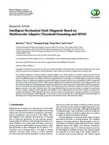
of data makes these fields endorse the concept and power of big data [1]–[3]. The big data not only promises to bring these fields new perspectives and challenges in processing and discovering valuable information [4], but also may prompt its power to affect other fields, like the field of condition monitoring and fault diagnosis of machines [5]. In modern industries, machines have become more automatic, precise and efficient than ever before [6]–[8], which makes their health condition monitoring more difficult. To fully inspect the health conditions of the machines, condition monitoring systems are used to collect real-time data from them, and big data are acquired by multiple sensors after the long-time operation. As the data is generally collected faster than it is analyzed by diagnosticians, how to effectively extract characteristics from mechanical big data and accurately identify the corresponding health conditions becomes an urgent research subject currently. Since intelligent fault diagnosis is able to rapidly and efficiently process massive collected signals and provide accurate fault diagnosis results, it may be a promising tool to handle the mechanical big data. Traditionally, the framework of intelligent fault diagnosis includes three main steps: signal acquisition, feature extraction and selection, and fault classification [9]–[11], as shown in Fig. 1(a). In the signal acquisition step, vibration signals have been extensively utilized since they provide the most intrinsic information about mechanical faults. In the second step, feature extraction aims to extract representative features from the collected signals based on signal processing techniques, like time-domain statistical analysis, Fourier spectral analysis and wavelet transformation [12]. Although these features characterize the mechanical health conditions, they may contain useless or insensitive information and affect the diagnosis results as well as computational efficiency. So feature selection is used to select sensitive features through dimension reduction strategies, such as principal component analysis (PCA), distance evaluation technique [13] and feature discriminant analysis [14]. In the fault classification step, the selected features are used to train artificial intelligence techniques like k-nearest neighbor (kNN), artificial neural networks and support vector machine (SVM) [15], and the mechanical health conditions are finally determined by these techniques. For instance, Lei et al. [16] used an improved distance evaluation technique to select six sensitive features from the time- and frequency-domain features, and these

0278-0046 (c) 2015 IEEE. Personal use is permitted, but republication/redistribution requires IEEE permission. See http://www.ieee.org/publications_standards/publications/rights/index.html for more information.


IEEE TRANSACTIONS ON INDUSTRIAL ELECTRONICS features were fed into ensemble adaptive neuro-fuzzy inference systems to classify the faults of bearings. Yu [17] presented a fault classification method for bearings in which eleven timeand frequency-domain features were used to represent different bearing faults and kNN was applied to classify the health conditions based on the features selected by local and nonlocal preserving projection. Amar et al. [18] proposed a feature enhancement procedure to obtain robust image features of vibration spectra and used an artificial neural network to diagnose the faults. A wavelet-spectrum technique was used to extract features by Liu et al. [19] and an enhanced neuro-fuzzy classifier was employed to classify bearing health conditions. It can be found that plenty of studies have been conducted on intelligent fault diagnosis and achieved good results [9]. These studies, however, may suffer three weaknesses as follows. First, traditional artificial intelligent techniques are unable to extract and organize the discriminative information from raw data directly. So lots of the actual effort in intelligent diagnosis methods goes into the design of feature extraction algorithms in order to obtain the representative features from the signals. Such processes take advantage of human ingenuity but largely depend on much prior knowledge about signal processing techniques and diagnostic expertise, which is time-consuming and labor-intensive. Second, the features are ordinarily extracted and selected according to a specific diagnosis issue and probably unsuitable for other issues. When handling a new diagnosis task, the feature extraction algorithms may need to be redesigned. Third, lacking a comprehensive understanding of mechanical big data, it is often difficult to ensure the extracted features carrying optimal information to classify the mechanical faults. Thus diagnosticians need to spend lots of time in analyzing these data and grasping their properties, which is tough work. To overcome these weaknesses, it would be highly desirable to adaptively learn the features from raw data using advanced artificial intelligent techniques, instead of extracting and selecting features manually. This would make intelligent fault diagnosis methods less dependent on the prior knowledge or human labor, so that novel applications could be done faster, and more importantly, to make mechanical fault diagnosis towards real artificial intelligence [20]. Unsupervised feature learning may hold the potential to overcome the aforementioned weaknesses in the traditional intelligent diagnosis methods. The basic idea behind unsupervised feature learning is that training artificial intelligence techniques can be viewed as learning a nonlinear function, which transforms the raw data from the original space into a feature space. So unsupervised feature learning is a set of algorithms studying how to well train the artificial intelligence techniques with the unlabeled raw data so as to automatically learn the discriminative features needed for classification [21]. When an unsupervised feature learning algorithm performs well, its learned features are able to capture some explanatory information hidden in the raw data, amplify the information important for discrimination and suppress irrelevant variations [22]. Unsupervised feature learning has been widely used in various fields, such as image classification [23], object

detection [24], speech recognition [25], and high-energy physic [26], etc., and state-of-the-art performances are obtained in these fields. Inspired by the idea of unsupervised feature learning, we present a new framework of intelligent fault diagnosis, as shown in Fig. 1(b). In this framework, the features are directly learned from mechanical raw signals and a classifier is used to classify the mechanical faults based on these learned features. The highlight of the framework is that the features are learned from the raw signals using a general-purpose learning procedure instead of being extracted by diagnosticians. The new framework releases us from the tough tasks of designing feature extraction algorithms and makes it easier to build a diagnosis system, thus this framework is more intelligent than the traditional one.

Fig.1. Intelligent fault diagnosis framework: (a) the traditional one, and (b) a new one.

The contributions of this paper are summarized as follows. 1) Following the new intelligent fault diagnosis framework, we propose a two-stage learning method. In the first learning stage, sparse filtering, which is viewed as a two-layer network, is used to learn representative features from the mechanical vibration signals. Then in the second learning stage, softmax regression, which is also a two-layer network, is trained to automatically classify the mechanical health conditions. Because of using a neural network to learn the features, the proposed method does not depend on prior knowledge and human labor and may be more suitable for processing massive signals in the field of condition monitoring and fault diagnosis. 2) Two diagnosis case studies are used to verify the proposed method. In the diagnosis case of motor bearings, the parameter selection of the proposed method and the effect of the amount of training data are thoroughly studied. Moreover, the proposed method is compared with related work for diagnosing the motor bearing dataset. The comparison results show the superiority of the proposed method. In the diagnosis case of locomotive bearings, the diagnosis results show that the proposed method could be employed to other diagnosis issues easily and effectively. 3) We try to explore a physical interpretation of sparse filtering in mechanical feature learning. The weight vectors of sparse filtering are well fitted by Gabor function, which means that these vectors can be viewed as Gabor-like filters. Adopting such a physical perspective on sparse filtering may provide an alternative way of understanding the role of sparse filtering in the unsupervised feature learning process.



IEEE TRANSACTIONS ON INDUSTRIAL ELECTRONICS The rest of this paper is organized as follows. In Section II, sparse filtering and softmax regression are briefly described. Section III details the proposed two-stage learning method. In Section IV and V, the diagnosis cases of two bearing datasets are studied separately using the proposed method. Finally, conclusions are drawn in Section VI. II. SPARSE FILTERING AND SOFTMAX REGRESSION A. Sparse Filtering Unsupervised feature learning techniques largely attempt to model the good approximation distribution of collected data [21], [27], including sparse autoencoders, restricted Boltzmann machines, sparse coding and so on. These methods may provide the good feature representations of mechanical signals. However, they often require the tuning of various parameters to perform well, which is a great challenge. For instance, the tunable parameters of the restricted Boltzmann machines are: number of features, weight decay, sparsity penalty, learning rate and momentum. Once these parameters are set inappropriately, the learned features may result in poor diagnosis accuracy [28]. Therefore, Ngiam et al. [29] proposed an unsupervised feature learning technique called sparse filtering. The key aspect of sparse filtering is that the only parameter required is the number of features. So sparse filtering does not necessarily include the parameter tuning and easily converges to an optimal solution [30]. Sparse filtering, viewed as an unsupervised two-layer network, optimizes the sparsity distribution of the features calculated by the collected data instead of modeling the distribution of the data. It tries to learn good features that satisfy three principles: population sparsity, lifetime sparsity and high dispersal. These principles have been explored in the field of neuroscience [31], [32]. Population sparsity means that each sample should be represented by only several active features, namely most of the features extracted from each sample should be zero. Lifetime sparsity means that each feature should be non-zero only for a few samples, which is beneficial to extract discriminative features. High dispersal is to encourage the distribution of features having similar statistics to each other and it will improve the generalization ability of the features [29]. As shown in Fig. 2, the inputs of sparse filtering are collected samples and the outputs are the learned features. Given a M training set {x i }i =1 , where x i ∈ ℜ N ×1 is a sample and M is the sample number, sparse filtering maps the samples onto their features f i ∈ ℜ L×1 using a weight matrix W ∈ ℜ N × L .

f l i = Wl T x i

(1)

i

where f l corresponds to the lth feature of the ith sample. Sparse filtering optimizes a function using l 2 - normalized features. It is noted that the lp - norm of t takes the form t

p

=

p

t1

p

+ L + tn

p

where t = [t1 , t 2 , L , t n ] .

The features f l i compose a feature matrix. We first normalize each row of the feature matrix by its l 2 - norm across all the samples ~ (2) fl = fl fl 2 . Then each column is normalized by its l 2 - norm , so that the features lie on the unit l2 - ball . ~ ~ fˆ i = f i f i (3) 2

Finally, the weight matrix W in (1) could be solved by optimizing a cost function constraining l1 - norm for each sample, which is shown as follows. M

minimize W

∑ i =1

fˆ i

(4) 1

As we know, l1- norm is commonly used to measure the sparsity of the elements [33], where sparse means that most of the elements are zero. The term fˆ i in (4) measures the 1

sparsity of the features of ith sample. As l 2 - normalized features fˆ i have been constrained to the unit l2 - ball , the cost function in (4) is minimized when these features are sparse. So the features could satisfy the property of population sparsity after the sparse filtering training. Since features are divided by their l2 - norm across the samples, the normalized features are equally active, implying that the contributions of these features are almost the same. Thus, the features are optimized for high dispersal. In addition, the features should have a lot of elements close to zero because of the population sparsity property. These elements could not be placed otherwise the features would be against the high dispersal property. Therefore, the features of a sample would have a lot of non-active elements so as to be the lifetime sparse. Sparse filtering can be extended to a nonlinear one by using an activation function, and the activation function g(⋅) = ⋅ is recommended [29]. So (1) is extended as f l i = g (Wl T x i ) . (5) By optimizing the cost function of the features in (5), the learned features are able to discover non-linear information from the input samples and have good generalization ability. More details of sparse filtering are described in [29]. B. Softmax Regression

Fig. 2. The architecture of sparse filtering.

In neural networks, softmax regression is often implemented at the final layer for multiclass classification [34]. It is easy to be implemented and is computed fast. Suppose that we have a training set {x i }i =1 with its label set {y i }i =1 where x i ∈ ℜ N ×1 M

We consider the situation that sparse filtering computes linear features for each sample.

M

and y i ∈ {1,2, L , K } . For each input sample x i , the model




Fig. 3. The proposed two-stage learning method: (a) illustration and (b) flowchart of training process.

attempts to estimate the probability p ( y i = k x i ) for each label of k = 1,2, L , K . Thus, the hypothesis of softmax regression will output a vector that gives K estimated probabilities of the input sample x i belonging to each label. Concretely, the hypothesis hθ ( x i ) takes the form:  p( y i = 1 x i ; θ )    i i  p( y = 2 x ; θ )  i hθ ( x ) =  = M    p( y i = K x i ; θ )  

1 K

∑e k =1

θ kT x i

e θ1T x i   θ2T x i  e   M   θ T xi  e K 

(6)

where θ = [θ1 , θ2 ,L, θ K ] are the parameters of the softmax T

K

regression model. It should be noticed that the term

∑e

θ kT x i

k =1

normalizes the distribution, so that the sum of the elements of hypothesis equals 1. Based on the hypothesis, the model is trained by minimizing the cost function J (θ ) .

  θ kT x i   λ K N M K 1 e ∑∑ 1 y i = k log K  + ∑∑ θ kl2 (7) J (θ ) = − M  i =1 k =1 2 k =1 l =1 θ lT x i  e ∑   l =1   where 1{} ⋅ denotes the indicator function returning 1 if the condition is true, and 0 otherwise; λ is the weight decay term. The weight decay term forces some of parameters of softmax regression to take values close to zero while permits other parameters to retain their relatively large values, thereby improving the generalization ability [35]. With the weight decay term (for any λ > 0 ), the cost function J (θ ) is strictly convex and the softmax regression model is guaranteed to have a unique solution theoretically [36]. Moreover, Softmax regression is a particular solution to the classification problem

{

}

assuming that a linear combination of the features of a sample can be used to determine the probability that the sample belongs to each health condition label, namely softmax regression provides probabilistic classification. III. THE TWO-STAGE LEARNING METHOD This section details the proposed two-stage learning method for intelligent fault diagnosis of machines. The illustration and flowchart of the method are shown in Fig. 3. In the first learning stage, sparse filtering is used to extract local discriminative features from raw vibration signals and the learned features of the signals are obtained by averaging these local features. In the second stage, softmax regression is applied to classify mechanical health conditions using the learned features. The vibration signals of machines are obtained under different health conditions. These signals compose the training M set {x i , y i }i =1 , where x i ∈ ℜ N ×1 is the ith sample containing N

vibration data points, y i is the health condition label. A. The First Learning Stage The first learning stage has the three following steps. We first train sparse filtering and obtain its weight matrix W . Then, the trained sparse filtering is used to capture the local features from each sample. Finally, these local features are averaged so as to obtain the learned features of each sample. Suppose that the input dimension of sparse filtering is N in and the output dimension of sparse filtering is N out . When training the sparse filtering model, we randomly sample Ns segments from the training samples. It means that the random segments are obtained using an overlapped manner. As shown in Fig. 4, these segments compose the unsupervised training set

{s }

j Ns j =1

where s j ∈ ℜ N in ×1 is the jth segment containing N in

data points. The set {s j }j =s1 is rewritten as a matrix form N




S ∈ ℜ N in × N s and pre-processed by whitening. The goal of whitening is to make the segments less correlated with each other and speed up the convergence of the sparse filtering training [37]. Whitening uses the eigenvalue decomposition of the covariance matrix

cov( S ) = EDE T (8) where E is the orthogonal matrix of eigenvectors of the covariance matrix cov(S ) and D is the diagonal matrix of its eigenvalues. So the whitened training segment set S white can be obtained. S white = ED −1 2 E T S (9) The sparse filtering model is trained by S white , and the trained weight matrix W is used to calculate the local features of the training samples. We alternately divide training samples into J segments, where J is an integer and equals N N in , namely x i is

{ }

divided to a segment set x ij

J j =1

N ×1 where x ij ∈ ℜ in . For each

x ij , we can get the local features f ji ∈ ℜ1× N

out

using the trained i

i

sparse filtering. Traditionally, the learned features f of x is obtained by combining these local features f ji in an aggregate way [38]. In other words, the local features are concatenated into one feature vector as the learned features.

[

f i = f1i , f 2i , L , f Ji

]

T

(10) In this paper, we use an average way instead of the aggregate way, and the learned feature is obtained as follows. T

1 J  (11) f i =  ∑ f ji   J j =1    Averaging is beneficial because it enhances discriminative features that the segments share with each other and suppresses random features caused by noise.

{}

M

it with the label set yi i =1 to train softmax regression. The softmax regression model computes the probability that the feature f i has the health condition labels y i as in (6). The sum of the probabilities over all class labels being 1 ensures that the right side in (6) defines a properly normalized distribution. After being trained, the maximum posterior probability in i hθ ( xi ) indicates which health condition label the feature f

belongs to. After the two learning stages, we use test samples to verify the proposed method. For each test sample, we first alternately divide it into segments. Then the trained sparse filtering model is used to obtain the local features from the segments. Next, the learned features of each test sample are obtained by averaging these local features. Finally, the health conditions of the test samples are decided by the trained softmax regression model using the learned features. IV. CASE STUDY Ⅰ: FAULT DIAGNOSIS OF MOTOR BEARINGS USING THE PROPOSED METHOD A. Data Description The motor bearing signals provided by Case Western Reserve University [39] are analyzed in this section. The vibration signals were collected from the drive end of a motor in the test rig under four different conditions: normal condition, outer race fault (OF), inner race fault (IF), and roller fault (RF). For OF, IF, and RF cases, vibration signals for three different severity levels (0.18, 0.36, and 0.53 mm) were separately collected. The signals were all collected under four load conditions (0, 1, 2 and 3 hp) and the sampling frequency was 12 kHz. These vibration signals compose the motor bearing dataset, which is used to verify the performance of the proposed method. The dataset contains ten bearing health conditions under the four loads, where the same health condition under different loads is treated as one class. There are 100 samples for each health condition under one load. Therefore, the motor dataset totally contains 4,000 samples, where each sample is a vibration signal of bearings containing 1,200 data points. B. Parameter Selection of the Proposed Method There are several parameters in the proposed method, i.e., the input dimension Nin and the output dimension N out of sparse

Fig. 4. Illustration of the training process of sparse filtering.

B. The Second Learning Stage

{ }

Once the learned feature set f i

M i =1

is obtained, we combine

filtering, and the weight decay term λ of softmax regression. We investigate the selection of these parameters respectively. It should be noted that 20 trials are carried out for each experiment in the following studies to reduce the effects of the randomness. First we investigate the selection of the input dimension Nin of sparse filtering. We randomly select 10% of samples to train the proposed method, where 20,000 segments are sampled from the training samples to train sparse filtering in the first learning stage, and the rest samples are used for testing. The output dimension N out = N in 2 and the weight decay term λ = 1E-5. The diagnosis results are shown in Fig. 5. In the figure, the time



IEEE TRANSACTIONS ON INDUSTRIAL ELECTRONICS averaged by 20 trials includes the training time and the testing time (the computation platform is a PC with an Intel I5 CPU and 8G RAM). Besides, the training accuracies and testing accuracies are also averaged by 20 trials, and the positive error bars show the standard deviations. It can be seen that all training accuracies are over 99.3% and testing accuracies are over 97.8%. It means that the proposed method is able to classify the ten health conditions of the motor bearing dataset with high accuracies using various input dimension of sparse filtering. But the larger the input dimension is, the more time the method spends. Considering that the testing accuracy of Nin = 100 is a little higher than others and the average time is low, we choose 100 as the input dimension Nin . Then we investigate the selection of the output dimension N out of sparse filtering. The diagnosis results are displayed in Fig. 6. When the output dimension is increasing, the accuracies are going higher and the corresponding standard deviations are continuously smaller. But the average time is growing linearly. It indicates that the selection of the output dimension is trade-off between the diagnosis accuracies and the spent time. Since the increasing of the accuracies is not obvious after N out equals 100, we choose 100 as the output dimension N out . Finally, we investigate the weight decay term λ of softmax regression. The diagnosis results are displayed in Fig. 7. It can be seen that the accuracies are low and their standard deviations are high when λ is too large. The reason is that the large λ forces too many parameters of softmax regression taking the values to zero. The accuracies and the standard deviations are steady after λ = 1E-5, so 1E-5 is chosen as the weight decay value in this paper.

Fig. 7. Diagnosis results using various weight decay terms.

C. Effect of the Data Number for Training After choosing the parameters of the proposed method, we study the effect of the number of the training data, i.e., the percentage of samples for training the proposed method, and the number of segments sampled from the training samples for training sparse filtering. In Fig. 8, it shows the diagnosis accuracies using various segment numbers when 10% of samples are randomly selected for training. It is seen that when the segment number goes larger, the testing accuracy is higher and the standard deviation is smaller. It should be noticed that the segments are unlabeled data and is obtained much easier than the labeled data, which means that the proposed method is able to take advantage of unsupervised learning and improve its diagnosis accuracy. However, the average time is increasing exponentially along with the increase of the segment number. To take the trade-off between the spent time and diagnosis accuracy, we use 20,000 segments for the motor bearing dataset.

Fig. 5. Diagnosis results using various input dimension of sparse filtering. Fig. 8. Diagnosis results using different segment numbers.

Fig. 6. Diagnosis results using various output dimension of sparse filtering.

The diagnosis results using the proposed method trained by different percentages of samples are shown in Fig. 9. It is certain that the testing accuracy increases and its standard deviation decreases with the rise of percentage of samples. It is seen from the figure that the proposed method diagnoses the ten health conditions of the motor bearing dataset with 95.2% accuracy using only 2% of samples for training. When the percentage increases to 10%, the testing accuracy is 99.66% with a small standard deviation of 0.19%. They indicate that the proposed method could perform well even in the situation of



IEEE TRANSACTIONS ON INDUSTRIAL ELECTRONICS lacking the labeled data. In the following studies, we use 10% of samples for training. In addition, it is seen from the Figs. 5, 6 and 8 that more computation cost of the proposed method is needed along with the increase of the architecture of sparse filtering and the amount of data used for training. But larger output dimension of sparse filtering and more training data imply the better diagnosis accuracies. So it is actually a trade-off choice in application of the proposed method.

Fig. 10. F-scores of the motor bearing dataset using the method without whitening, the method with aggregate features, and the proposed method.

E. Comparing with Related Work

Fig. 9. Diagnosis results using the proposed method trained by different percentages of samples.

D. Necessity of Whitening and Local Feature Averaging In the proposed two-stage learning method, it is noticed that whitening is used in the training process of sparse filtering and the learned features are averaged by the local features instead of being aggregated. Here we study the necessity of the whitening and the local feature averaging. We diagnose the motor bearing dataset using the method without whitening and the method with the aggregate features calculated by (10). To compare their performances with that of the proposed method, F-score is adopted [40], which is a common used criterion measuring the performance of a classification method. It considers both the precision and the recall of the results, where precision is a function of the correctly classified samples (true positives, TP) and samples misclassified as positives (false positives, FP), and recall is a function of TP and its misclassified samples (false negatives, FN). F-score reaches its best value at 1 and worst score at 0.

p=

TP TP and r = TP + FP TP + FN p×r F-score = 2 × p+r

(12) (13)

In Fig. 10, the F-scores of the motor bearing dataset using the three methods are shown, where each F-score is averaged by 20 trials. It can be seen that the F-scores using the proposed method range from 0.993 to 1, whereas the F-scores using the method without whitening range from 0.907 to 1 and the F-scores using the method with aggregate features range from 0.929 to 1. For most health conditions, the proposed method obtains higher F-scores than the other two methods, which means that the proposed method performs better. Therefore, the whitening and the local feature averaging are both necessary for the proposed method.

Different from the methods following the traditional intelligent fault diagnosis framework, the proposed method directly learns features from the raw vibration signals using an artificial intelligence technique and classifies the mechanical health conditions based on the learned features. To show the effectiveness of the proposed method, we compare it with the methods in the related work using the same motor bearing dataset. The comparisons are displayed in Table I. Du et al. [41] proposed a method based on wavelet leaders multi-fractal features and SVM. When their method was employed to classify the ten health conditions of the motor bearings, the accuracy of 88.9% was got. In [42], nine time-domain statistical features combined with six features about the percentage of energy corresponding to wavelet coefficients were used to represent ten bearing health conditions under the load of 3 hp. Then these parameters were classified by the trace ratio linear discriminant analysis trained with 10% of samples, and finally 92.5% diagnosis accuracy was achieved. A method [43] using 19 time-domain and frequency-domain features combined with semi-supervised self-organizing map was proposed by Li et al. The method was used to classify the bearings with multiple roller defects (0, 0.178, 0.355, and 0.533 mm in diameter, respectively) and the classification accuracy of 95.8% was obtained. Zhang et al. [44] proposed a bearing diagnosis method integrating permutation entropy, ensemble empirical mode decomposition and optimized SVM. The method was used to distinguish eleven health conditions and got 97.91% testing accuracy. Compared with the methods above, the proposed method is trained by a lower percentage of samples and obtains a higher accuracy. It is known that obtaining discriminative features is a crucial step for intelligent fault diagnosis. In the compared methods, the feature extraction needs diagnosticians to spend lots of time in analyzing collected signals and grasping their properties based on many signal processing techniques, like band-pass filtering, wavelet analysis and ensemble empirical mode decomposition. Although the extracted features manually concentrate the information important for classification and discard the variations irrelevant, in-depth knowledge on



IEEE TRANSACTIONS ON INDUSTRIAL ELECTRONICS mechanical vibration signals and much diagnostic expertise is essential. Such processes take advantage of human ingenuity but largely depend on human labor. As the collected data goes larger, it is increasingly difficult to manually design the feature extraction algorithm. Contrarily, the proposed method learns the features adaptively from the raw vibration signals with a neural network, which makes it less dependent on prior knowledge and human labor. Additionally, the unlabeled data is much more easily obtained than the labeled data. The proposed method can take advantage of unsupervised learning and improve the diagnosis accuracies with the increasing number of the unlabeled data, which is shown in Fig. 8. So based on the proposed method, new applications of processing massive signals could be achieved easily. TABLE I CLASSIFICATION COMPARISON OF THE MOTOR BEARING DATASET No. of Training Load (hp) No. of health Testing Methods samples condition accuracy [41] 75% 0 10 88.9% [42] 10% 3 10 92.5% 4 95.8% [43] 40% 0, 1, 2, 3 11 97.91% [44] 40% 0, 1, 2, 3 Proposed 10% 0, 1, 2, 3 10 99.66%

F. Sparse Filtering Shares a Physical Interpretation As shown in Fig. 3(a), sparse filtering is used to extract local discriminative features from raw vibration signals and the learned features of the signals are obtained by averaging the local features. Since the learned features are high-dimensional vectors, they cannot be plotted directly. So PCA is implemented on the learned features, and their first three principal components (PCs) are shown in Fig. 11. It is seen that most features of the same health condition are gathered in the corresponding cluster and most features of the different health conditions are separated. This reveals that the proposed method could learn the features irrespective of the varying loads.

neural network weights learned in mechanical intelligent fault diagnosis and explore why sparse filtering could learn the features adaptively. We rewrite (1) as the inner product form in (14). It indicates that the value of the lth output neuron is calculated by the inner product operation of the input signal x i and the weight vector Wl . So sparse filtering can be interpreted to measure the similarity between the input signals and a series of weight vectors, like wavelet transform providing estimates of similarity between the signals and basis functions [45]. The sparse filleting features in (5) just transform the similarity into a nonlinear form.

f l i = Wl T x i = Wl , x i

(14)

We randomly select 12 weight vectors of sparse filtering, as shown in Fig. 12(a). It is found that the weight vectors show striking similarities to the one-dimensional Gabor filters that serve as excellent band-pass filters for signals. So we fit each weight vectors using Gabor function f (d ) [46], [47].

 (d − D )2   cos(2πω(d − D ) + φ ) + B (15) f (d ) = A exp −  2σ 2   where A , ω and φ are the amplitude, spatial frequency and phase of the cosine term, respectively, σ is the standard deviation of the Gaussian, D is a position offset, and B is an offset parameter. It can be seen from Fig. 12(a) that the weight vectors are well fitted and their Fourier transforms are shown in Fig. 12(b). It is found that most of the weight vectors have narrow spectral bandwidths. Therefore, the trained weight vectors can be compared directly to the Gabor filters, which give a physical interpretation to sparse filtering.

Fig. 11. Scatter plots of principal components for the learned features of the motor bearing dataset.

Traditionally, a neural network is regarded as a black box and few papers in the field of fault diagnosis try to explain the properties of the weights learned in the neural network. So it is not easy to understand the roles of neural network in fault diagnosis. In this paper, we try to discover the patterns of the

Fig. 12. (a) Selected weight vectors for the motor bearing dataset and the fitted vectors by Gabor function, and (b) the corresponding Fourier transforms.



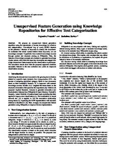
IEEE TRANSACTIONS ON INDUSTRIAL ELECTRONICS V. CASE STUDY Ⅱ: FAULT DIAGNOSIS OF LOCOMOTIVE BEARINGS USING THE PROPOSED METHOD The vibration signals of locomotive bearings were collected from a test bench which consisted of a hydraulic motor, two supporting pillow blocks, a hydraulic cylinder, a hydraulic radial load application system, and a tachometer for shaft speed measurement. The tested bearings were installed in the hydraulic motor driven mechanical system and loaded by the hydraulic cylinder. Accelerometers were mounted on the load module to measure the vibration signals. The sampling frequency is 12.8 kHz. The locomotive bearing dataset involves seven different health conditions under four different loads varying around 9800 N. The seven health conditions are: normal condition (N), slight rub fault in the outer race (OF1), serious flaking fault in the outer race (OF2), slight rub fault in the inner race (IF), roller rub fault (RF), concurrent faults in the outer race and roller (ORF), and concurrent faults in the inner race and roller (IRF). There are 273 samples for each health condition under one load. The dataset totally contains 7,644 samples and each sample is a vibration signal containing 1,200 data points. To classify the health conditions of the locomotive bearings, the proposed method is trained by 10% of samples where 40,000 segments are used to train sparse filtering and the rest samples are applied to test the performance. The input dimension and output dimension of sparse filtering are 100 and 50, respectively. The weight decay term is 1E-5. The average testing accuracy and the corresponding standard deviation of 20 trials are 99.0% and 0.19%, respectively. It means that the proposed method could distinguish not only single faults like IF and RF but also the concurrent faults like ORF and IRF with high accuracy and small standard deviation. To show more details about the diagnosis information, the confusion matrix of the proposed method on the locomotive bearing dataset is presented in Fig. 13. As we can see, the proposed method misclassifies 3.45% of testing samples of the ORF as the IRF and 2.29% of testing samples of the IRF as the ORF. The reason may be that the IRF and ORF both contain the roller fault and the signals of the two concurrent faults are similar, which makes it more difficult to distinguish the two health conditions than other conditions.

The scatter plots of principal components of the learned features are shown in Fig. 14. It is noticed that the learned features of the five single faults characterizing the same health conditions are clustered well and each cluster is separated, whereas a few learned features of the ORF and IRF mixed with each other. This corresponds to the diagnosis results displayed in the confusion matrix.

Fig. 14. Scatter plots of principal components for the learned features of the locomotive bearing dataset.

Twelve weight vectors of the trained sparse filtering for the locomotive bearing dataset are shown in Fig 15(a). These weight vectors are also fitted by the Gabor function in (15). The fitted weight vectors and their Fourier transforms are shown in Fig. 15. As same as the case study of the motor bearing dataset, these weights are time-localized and have narrow spectral bandwidths. Therefore, it confirms that sparse filtering on the locomotive bearing dataset shares the physical interpretation.

Fig. 15. (a) Selected weight vectors for the locomotive bearing dataset and the fitted vectors by Gabor function, and (b) the corresponding Fourier transforms. Fig. 13. Confusion matrix of the locomotive bearing dataset.



IEEE TRANSACTIONS ON INDUSTRIAL ELECTRONICS VI. CONCLUSIONS It would be desirable to make intelligent fault diagnosis less dependent on prior knowledge and diagnostic expertise when processing mechanical big data, especially in the feature extraction step. So this paper presents a two-stage learning method based on the idea of unsupervised feature learning. In the method, sparse filtering adaptively learns features that capture discriminative information from vibration signals in an unsupervised way. Then the features are fed to softmax regression to classify health conditions in a supervised manner. Through the case studies of the two bearing datasets, it is shown that the proposed method adaptively learns features from raw signals for various diagnosis issues and is superior to the existing methods in fault diagnosis of the motor bearing dataset. The proposed method is able to take advantage of unsupervised learning and improve its diagnosis accuracy along with the increase of the number of the unlabeled data. Moreover, a physical interpretation is explored to the weight vectors of sparse filtering and these vectors show similar properties to those of the Gabor filters. Adopting the physical interpretation to sparse filtering may provide perspectives on how unsupervised feature learning techniques deal with mechanical signals. So in future work, the properties of the neural network weights will be deeply studied through unsupervised feature learning, in order that we can bridge the gap between manual feature extraction using signal processing techniques and feature learning using artificial intelligence techniques. Additionally, it has been a hot topic that applies neural networks in the field of industrial system control [48]–[51], so investigating the application of an unsupervised neural network in the field will be an interesting future research subject. There may be some guidance on the utilization of the proposed method. First, it is advised to use a large amount of unlabeled data to train sparse filtering. The more data we use, the better the learned features will be. Second, the whitening process is necessary because it is able to speed up the convergence of the sparse filtering training. It is noted that the mean value of each segment should be zero before whitening. Finally, it is more effective to use the strategy of local feature averaging in the diagnosis cases of lacking the labeled data for the final classification. In a word, the amount of labeled and unlabeled data both determines the performance of the proposed method, which makes it a promising tool for fault diagnosis under mechanical big data.

[6]

[7]

[8]

[9]

[10]

[11]

[12]

[13]

[14]

[15]

[16]

[17]

[18]

[19]

[20]

[21] [22] [23]

[24]

[25]

REFERENCES [1] [2] [3] [4] [5]

S. J. Qin, “Process data analytics in the era of big data,” AIChE Journal, vol. 60, no. 9, pp. 3092-3100, Jul. 2014. F. Frankel, and R. Reid, “Big data: Distilling meaning from data,” Nature, vol. 455, no. 7209, pp. 30-30, Sep. 2008. X.-W. Chen, and X. Lin, “Big data deep learning: Challenges and perspectives,” IEEE Access, vol. 2, pp. 514-525, May 2014. X. Wu, X. Zhu, G.-Q. Wu, and W. Ding, “Data mining with big data,” IEEE Trans. Knowl. Data Eng., vol. 26, no. 1, pp. 97-107, Jan. 2014. S. Yin, and O. Kaynak, “Big data for modern industry: challenges and trends,” Proc. IEEE, vol. 103, no. 2, pp. 143-146, Feb. 2015.

[26]

[27]

[28]

W. Qiao, and D. Lu, “A survey on wind turbine condition monitoring and fault diagnosis, ” IEEE Trans. Ind. Electron., vol. 62, no. 10, pp. 6536-6545, Oct. 2015. Y. Lei, J. Lin, M. J. Zuo, and Z. He, “Condition monitoring and fault diagnosis of planetary gearboxes: A review,” Measurement, vol. 48, pp. 292-305, Feb. 2014. J. Yu, “A nonlinear probabilistic method and contribution analysis for machine condition monitoring,” Mech. Syst. Signal Process., vol. 37, no. 1, pp. 293-314, May 2013. K. Worden, W. J. Staszewski, and J. J. Hensman, “Natural computing for mechanical systems research: A tutorial overview,” Mech. Syst. Signal Process., vol. 25, no. 1, pp. 4-111, Jan. 2011. Y. Shatnawi, and M. Al-khassaweneh, “Fault diagnosis in internal combustion engines using extension neural network,” IEEE Trans. Ind. Electron., vol. 61, no. 3, pp. 1434-1443, Mar. 2014. M. D. Prieto, G. Cirrincione, A. G. Espinosa, J. A. Ortega, and H. Henao, “Bearing fault detection by a novel condition-monitoring scheme based on statistical-time features and neural networks,” IEEE Trans. Ind. Electron., vol. 60, no. 8, pp. 3398-3407, Aug. 2013. D. You, X. Gao, and S. Katayama, “WPD-PCA-based laser welding process monitoring and defects diagnosis by using FNN and SVM,” IEEE Trans. Ind. Electron., vol. 62, no. 1, pp. 628-638, Jan. 2015. Y. Lei, Z. He, Y. Zi, and X. Chen, “New clustering algorithm-based fault diagnosis using compensation distance evaluation technique,” Mech. Syst. Signal Process., vol. 22, no. 2, pp. 419-435, Feb. 2008. M. Kang, J. Kim, J.-M. Kim, A. C. Tan, E. Y. Kim, and B.-K. Choi, “Reliable Fault Diagnosis for Low-Speed Bearings Using Individually Trained Support Vector Machines With Kernel Discriminative Feature Analysis,” IEEE Trans. Power Electron., vol. 30, no. 5, pp. 2786-2797, May 2015. S. Yin, S. X. Ding, X. Xie, and H. Luo, “A review on basic data-driven approaches for industrial process monitoring,” IEEE Trans. Ind. Electron., vol. 61, no. 11, pp. 6418-6428, Nov. 2014. Y. Lei, Z. He, Y. Zi, and Q. Hu, “Fault diagnosis of rotating machinery based on multiple ANFIS combination with GAs,” Mech. Syst. Signal Process., vol. 21, no. 5, pp. 2280-2294, Jul. 2007. J. Yu, “Local and nonlocal preserving projection for bearing defect classification and performance assessment,” IEEE Trans. Ind. Electron., vol. 59, no. 5, pp. 2363-2376, May 2012. M. Amar, I. Gondal, and C. Wilson, “Vibration Spectrum Imaging: A Novel Bearing Fault Classification Approach,” IEEE Trans. Ind. Electron., vol. 62, no. 1, pp. 494-502, Jan. 2015. J. Liu, W. Wang, and F. Golnaraghi, “An enhanced diagnostic scheme for bearing condition monitoring,” IEEE Trans. Instrum. Meas., vol. 59, no. 2, pp. 309-321, Feb. 2010. Y. Bengio, A. Courville, and P. Vincent, “Representation learning: A review and new perspectives,” IEEE Trans. Pattern Analysis and Machine Intelligence, vol. 35, no. 8, pp. 1798-1828, Aug. 2013. A. Coates, A. Y. Ng, and H. Lee, “An analysis of single-layer networks in unsupervised feature learning,” in Proc. AISTATS, 2011, pp. 215-223. Y. LeCun, Y. Bengio, and G. Hinton, “Deep learning,” Nature, vol. 521, no. 7553, pp. 436-444, May 2015. K. Yu, Y. Lin, and J. Lafferty, “Learning image representations from the pixel level via hierarchical sparse coding,” in Proc. IEEE Conf. Comput. Vis. Pattern Recognit., 2011, pp. 1713-1720. M. A. Ranzato, F. J. Huang, Y.-L. Boureau, and Y. LeCun, “Unsupervised learning of invariant feature hierarchies with applications to object recognition,” in Proc. IEEE Conf. Comput. Vis. Pattern Recognit., 2007, pp. 1-8. G. Hinton, L. Deng, D. Yu, G. E. Dahl, A.-r. Mohamed, N. Jaitly, A. Senior, V. Vanhoucke, P. Nguyen, and T. N. Sainath, “Deep neural networks for acoustic modeling in speech recognition: The shared views of four research groups,” IEEE Signal Processing Mag., vol. 29, no. 6, pp. 82-97, Nov. 2012. P. Baldi, P. Sadowski, and D. Whiteson. Searching for exotic particles in high-energy physics with deep learning. Nature Commun., vol. 5, no. 4308, pp. 1-9, Jul. 2014. G. Hinton, and R. Salakhutdinov, “Reducing the dimensionality of data with neural networks,” Science, vol. 313, no. 5786, pp. 504-507, Jul. 2006. G. Hinton, “A practical guide to training restricted Boltzmann machines,” in Neural Networks: Tricks of the Trade, K.-R. Muller, G. Montavon, and G.B. Orr, Eds., Springer, 2013.



IEEE TRANSACTIONS ON INDUSTRIAL ELECTRONICS [29] J. Ngiam, Z. Chen, S. A. Bhaskar, P. W. Koh, and A. Y. Ng, “Sparse filtering,” in Proc. Neural Information and Processing Systems, 2011, pp. 1125-1133. [30] K. B. Raja, R. Raghavendra, V. K. Vemuri, and C. Busch, “Smartphone based visible iris recognition using deep sparse filtering,” Pattern Recogn. Lett., vol. 57, pp. 33-42, May 2015. [31] D. J. Field, “What is the goal of sensory coding?,” Neural Comput., vol. 6, no. 4, pp. 559-601, Jul. 1994. [32] B. Willmore, and D. J. Tolhurst, “Characterizing the sparseness of neural codes,” Network: Comput. Neural Syst., vol. 12, no. 3, pp. 255-270, 2001. [33] R. G. Baraniuk, “Compressive sensing,” IEEE Signal Processing Mag., vol. 24, no. 4, pp. 118-120, Jul. 2007. [34] J. Behley, V. Steinhage, and A. Cremers, “Laser-based segment classification using a mixture of bag-of-words,” in Proc. IEEE Int. Conf. Intell. Robots Syst., 2013, pp. 4195-4200. [35] J. Han, D. Zhang, S. Wen, L. Guo, T. Liu, and X. Li. (2015, Feb.). Two-stage learning to predict human eye fixations via SDAEs. IEEE Trans. Cybernetics [Online]. Available: http://ieeexplore.ieee.org/xpls/abs_all.jsp?arnumber=7051244 [36] C. Bielza, V. Robles, and P. Larrañaga, “Regularized logistic regression without a penalty term: An application to cancer classification with microarray data,” Expert Syst. Appl., vol. 38, no. 5, pp. 5110-5118, May 2011. [37] A. Hyvärinen, and E. Oja, “Independent component analysis: algorithms and applications,” Neural networks, vol. 13, no. 4, pp. 411-430, Jun. 2000. [38] N. Jaitly, and G. Hinton, “Learning a better representation of speech soundwaves using restricted boltzmann machines,” in Proc. Int. Conf. Acoust. Speech Signal Process., 2011, pp. 5884-5887. [39] X. Lou and K. a Loparo, “Bearing fault diagnosis based on wavelet transform and fuzzy inference,” Mech. Syst. Signal Process., vol. 18, no. 5, pp. 1077–1095, Sep. 2004. [40] M. Sokolova, N. Japkowicz, and S. Szpakowicz, “Beyond accuracy, F-score and ROC: a family of discriminant measures for performance evaluation,” in Proc. AI 2006: Advances in Artificial Intelligence, 2006, pp. 1015-1021. [41] W. Du, J. Tao, Y. Li, and C. Liu, “Wavelet leaders multifractal features based fault diagnosis of rotating mechanism,” Mech. Syst. Signal Process., vol. 43, no. 1, pp. 57-75, Feb. 2014. [42] X. Jin, M. Zhao, T. W. Chow, and M. Pecht, “Motor bearing fault diagnosis using trace ratio linear discriminant analysis,” IEEE Trans. Ind. Electron., vol. 61, no. 5, pp. 2441-2451, May 2014. [43] W. Li, S. Zhang, and G. He, “Semisupervised distance-preserving self-organizing map for machine-defect detection and classification,” IEEE Trans. Instrum. Meas., vol. 62, no. 5, pp. 869-879, May 2013. [44] X. Zhang, Y. Liang, and J. Zhou, “A novel bearing fault diagnosis model integrated permutation entropy, ensemble empirical mode decomposition and optimized SVM,” Measurement, vol. 69, pp. 164-179, Jun. 2015. [45] Z. R. Struzik, and A. Siebes, “The Haar wavelet transform in the time series similarity paradigm,” in Proc. 3rd Eur. Conf. Principles Data Mining Knowl. Discovery, 1999, pp. 12-22. [46] E. C. Smith, and M. S. Lewicki, “Efficient auditory coding,” Nature, vol. 439, no. 7079, pp. 978-982, Feb. 2006. [47] G. Masson, C. Busettini, and F. Miles, “Vergence eye movements in response to binocular disparity without depth perception,” Nature, vol. 389, no. 6648, pp. 283-286, Sep. 1997. [48] J. Qiu, G. Feng, and H. Gao, “Fuzzy-model-based piecewise H-infinity static output feedback controller design for networked onlinear systems,” IEEE Trans. Fuzzy Syst., vol. 18, no. 5, pp. 919-934, Oct. 2010. [49] T. Wang, H. Gao, and J. Qiu. (2015, Apr.). A combined adaptive neural network and nonlinear model predictive control for multirate networked industrial process control. IEEE Trans. Neural Netw. Learn. Syst. [Online]. Available: http://ieeexplore.ieee.org/xpl/articleDetails.jsp?arnumber=7087381 [50] H. Li, S. Yin, Y. Pan, and H. K. Lam, “Model reduction for interval type-2 Takagi–Sugeno fuzzy systems,” Automatica, vol. 61, pp. 308-314, Nov. 2015. [51] J. Qiu, S. X. Ding, H. Gao, and S. Yin. (2015, Jul.). Fuzzy-model-based reliable static output feedback H-infinity control of nonlinear hyperbolic PDE systems. IEEE Trans. Fuzzy Syst. [Online]. Available: http://ieeexplore.ieee.org/xpls/abs_all.jsp?arnumber=7161345

Yaguo Lei (M’15) received the B.S. and Ph.D. degrees in mechanical engineering from Xi’an Jiaotong University, Xi’an, China, in 2002 and 2007, respectively. He is currently a Full Professor of mechanical engineering at Xi’an Jiaotong University. Prior to joining Xi’an Jiaotong University in 2010, he was a Postdoctoral Research Fellow with the University of Alberta, Edmonton, AB, Canada. He was also an Alexander von Humboldt Fellow with the University of Duisburg-Essen, Duisburg, Germany. His research interests focus on machinery condition monitoring and fault diagnosis, mechanical signal processing, intelligent fault diagnostics, and remaining useful life prediction. Dr. Lei is a member of the American Society of Mechanical Engineers; a Senior Member of the Chinese Mechanical Engineering Society; and an Editorial Board Member of Neural Computing and Applications, Advances in Mechanical Engineering, The Scientific World Journal, International Journal of Mechanical Systems Engineering, Chinese Journal of Engineering, International Journal of Applied Science and Engineering Research, etc. Feng Jia is currently working toward the Ph.D. degree in mechanical engineering at the State Key Laboratory for Manufacturing System Engineering, Xi’an Jiaotong University, P. R. China. He received the B.S. and M.S. degree in mechanical engineering from Taiyuan University of Technology, P. R. China, in 2011 and 2014, respectively. His research interests include machinery condition monitoring and fault diagnosis, intelligent fault diagnostics of rotating machinery. Jing Lin received his B.S., M.S. and Ph.D. degrees from Xi’an Jiaotong University, P. R. China, in 1993, 1996 and 1999, respectively, all in mechanical engineering. He is currently a Professor with the State Key Laboratory for Manufacturing Systems Engineering, Xi’an Jiaotong University. From July 2001 to August 2003, he was a Postdoctoral Fellow with the University of Alberta, Edmonton, AB, Canada, and a Research Associate with the University of Wisconsin–Milwaukee, Milwaukee, WI, USA. From September 2003 to December 2008, he was a Research Scientist with the Institute of Acoustics, Chinese Academy of Sciences, Beijing, China, under the sponsorship of the Hundred Talents Program. His current research directions are in mechanical system reliability, fault diagnosis, and wavelet analysis. Dr. Lin was a recipient of the National Science Fund for Distinguished Young Scholars in 2011. Saibo Xing is currently working for the Ph.D. degree in mechanical engineering from Xi’an Jiaotong University, P. R. China and received the B.S. degree in material science and engineering from Xi’an Jiaotong University, in 2015. He graduated from Hsue-shen Tsien Experimental Class majoring in material science and engineering, and became the graduated student without examination majoring in mechanical engineering. His research interests focus on intelligent fault diagnostics and prognostics of rotating machinery. Steven X. Ding received the Ph.D. degree in electrical engineering from the Gerhard-Mercator University of Duisburg, Duisburg, Germany, in 1992. From 1992 to 1994, he was a Research and Development engineer at Rheinmetall GmbH, Dusseldorf, Germany. From 1995 to 2001, he was a professor of control engineering at the University of Applied Science Lausitz in Senftenberg, Germany, and served as vice president of this university during 1998-2000. He is currently a full professor of control engineering and the head of the Institute for Automatic Control and Complex Systems (AKS) at the University of Duisburg-Essen, Duisburg, Germany. His research interests include model-based and data-driven fault diagnosis, fault tolerant systems, real-time control, and their application in industry with a focus on automotive systems and chemical processes.
