Plastic deformation of crystals is the result of dislocation motion. ... the second part of this paper we show a Finite Element Method application of a 3D continuum theory of curved .... The gradient of such a smooth vector field âu , denoted by ... matrix form and the Cartesian coordinates for β we obtain. : x x x y y y z z z u u u x.
78
Scientific Technical Review, 2011,Vol.61,No.3-4,pp.78-88 UDK: 548:544.032.2:624.011.78 COSATI: 11-06, 20-12
An Introduction to the Theory of Three Dimensional Curved Dislocations Milan Cajić1) Plastic deformation of crystals is the result of dislocation motion. Owing to the long-range nature of dislocation interactions, the development of a continuum theory of plasticity, based on the averaged dynamics of dislocation systems, represents a difficult mathematical problem. Here, we summarize current advances in the field of sizedependent continuum plasticity of crystals, based on the dislocation density measure which is able to account for the evolution of systems of three-dimensional curved dislocations. In the first part of the current work we introduce a self-consistent theory and its dislocation density measure with a definition and an evolution equation which is a direct generalization of the definition and the kinematic evolution equation of the Kröner-Nye dislocation density tensor. In the second part of this paper we show a Finite Element Method application of a 3D continuum theory of curved dislocations, which is based on the definition of dislocation density in higher dimensional state space containing dislocation orientation information Key words: crystallography, continuum mechanics, crystal deformation, plastic deformation, deformation tensor, density tensor, dislocation.
T
Introduction
HE first suggestion of dislocations was provided by observations [1], [2] in the nineteenth century that the plastic deformation of metals proceeded by the formation of slip bands, wherein one portion of a specimen sheared with respect to another. Initially, the interpretation of this phenomenon was obscure, but with the discovery that metals were crystalline, it was appreciated that such a slip must represent the shearing of one portion of a crystal with respect to another on a crystallographic plane [3]. Continuum theories of dislocations have already been introduced in the 1950s independently by Kroner [4], Nye [5], Bilby and co-workers [6] and Kondo [7]. Their theories were founded on the so-called Kröner-Nye dislocation density tensor, which served as a measure for the defect state of a crystal. However, already then it was obvious that the dislocation density tensor as an averaged object does not carry enough information about the dislocation state to deduce the rate of plastic deformation from it (for details see the third chapter). In general, it is not possible to build a closed theory of plasticity solely on the Kröner-Nye dislocation density tensor. However, such a formulation can be used in the case of a single dislocation as singular densities and in special cases where dislocations form smooth bundles of parallel lines of the same orientation (e.g. as done by Acharya [8], [9], [10] and by Sedláček at al. [11]). Only in these cases the density function ρ coincide with the total dislocation density and the averaged line direction gives the true direction of dislocation lines. Using this dislocation density measure in more general situations leads to non-closed formulations which need to be ’patched up’ by phenomenological assumptions. Another approach in terms of higher-dimensional density measure was proposed by Kosevich [12] and similarly by 1)
Mathematical Institute SANU, Kneza Mihaila 36, 11000 Belgrade, SERBIA
El-Azab [13]. The first one defines dislocation densities in a space which includes parameters characterizing the line orientation as an independent variable and the second one extended the statistical mechanics to systems of curved dislocation lines by using densities that evolve in a higher dimensional state space. According to the observations in [21], the measures of these two systems are not capable of distinguishing a distribution of circular loops from the distribution of randomly oriented dislocation straight lines in a plane with the same Burgers vector. The recent study by Hochrainer [14] introduced the Extended Continuum Theory (ECT) which is applicable to very general dislocation configurations. In this theory, mathematical foundations required for transferring the methods of statistical mechanics consistently with three dimensional systems of curved dislocations have been formulated. In the following text, we will briefly introduce the ECT. For a complete introduction and derivation of this theory, the reader is referred to [14] and [15]. According to the observation in [16], advances in addressing a problem of the formulation of a size-dependent continuum theory based on the mechanics of discrete dislocations have been accomplished and given in a rigorous mathematical form. However, the problem of describing grain boundaries and interfaces as well as their interactions with dislocations still has many unsolved issues. Mesarović has analyzed the second problem within the continuum framework and with a particular emphasis on the slip relaxation at interfaces (for details see e.g. [16, 17, 18]). All these approaches, outlined above, provide a general framework to study dislocation kinematics and dynamics, dislocation density evolution, description of grain boundaries and interfaces and their reactions with dislocations. Nevertheless, the subject of this
79
CAJIĆ,M.: AN INTRODUCTION TO THE THEORY OF THREE DIMENSIONAL CURVED DISLOCATIONS
communication is much narrower and shows a short review of the ECT theory and the FEM application of an improved model of the Kröner-Nye dislocation density measure (ECT) in a single glide situation. In the current paper, we use the following definitions and conventions: ∇ denotes the gradient operator, x1 and x2 are the spatial plane coordinates, and with φ we denote the third dimension in a configuration space which physically represents the dislocation line orientation (for a more detailed description see the third chapter). Accordingly, with the capitalized DIV we denote the divergence operator which is operating in a higher-dimensional space which includes the orientation φ and it is written as DIV : = ⎛⎜ ∂ , ∂ , ∂ ⎞⎟ . ⎝ ∂x1 ∂x2 ∂φ ⎠
The
small-lettered
div is
the
divergence operator in a spatial plane div: = ⎛⎜ ∂ , ∂ ⎞⎟ . The ⎝ ∂x1 ∂x2 ⎠ Laplace operator Δ is given by the gradient of divergence and introduces the second derivative T
Δ: = grad ⎜⎛ ∂ , ∂ , ∂ ⎟⎞ ⎝ ∂x1 ∂x2 ∂φ ⎠
The tensors are denoted in bold-face letters and scalar quantities are written in non-bold ones, while curl denotes the rot-operator. The vector product is denoted by × , and the tensor product by ⊗ . The symmetric part of a matrix M of the second rank tensor mij (for example) can be obtained by the
S = 1 ( M + M T ) , where 2
M
T
is the
transpose of a matrix.
Consider a material distortion β as β: = ∇ u
( )
β = β pl + β el
(3)
and the same applies to the strain tensor
ε = ε pl + ε el
(4)
The relation between the elastic tensor and the local stress, obtained by the double contraction of two tensors, is given in the Cartesian coordinates
σ ij = Cijkl ε elkl
(5)
where Cijkl is the forth order tensor of the material elasticity constant and ε elkl is the elastic part of the strain tensor. We write Navier-s balance equations (also in the Cartesian coordinates) as
∂σ x τ yx ∂τ zx + + + XV ' = 0 ∂x ∂y ∂z
τ xy = τ yx
∂τ xy ∂σ y ∂τ zy + + + YV ' = 0 ∂x ∂y ∂z
τ xz = τ zx
∂τ xy ∂σ y ∂τ zy + + + YV ' = 0 ∂x ∂y ∂z
τ xz = τ zx
(6)
where σ i and τ ij ( i, j = x, y , z ) are the normal and the tangential components of the local stress tensor σ ij (see ref. [19] by Rašković or [20] by Hedrih (Stevanović)). In the absence of the volume body and the inertial forces ( X V ' , YV ' , ZV ' ), we obtain
Elasto-plasticity for small strains
G where u u, t
In the small-strain approximation, the material distortion (see ref. [4] by Kröner) can be additionally decomposed into a plastic and an elastic part
(1)
is a continuous and differentiable material
displacement field, which usually characterizes the G deformation of a body in continuum mechanics, and u is G G G G the displacement vector with a form u = u x i + u y j + u z k (see ref. [19] by Rašković or [20] by Hedrih (Stevanović)). The gradient of such a smooth vector field ∇u , denoted by β , in some literature (in ref. [4] by Kröener, for example) is called the distortion tensor or, in references mentioned above, it is called the functional matrix. However, in a matrix form and the Cartesian coordinates for β we obtain
∂σ x τ yx ∂τ zx + + =0 ∂x ∂y ∂z
τ xy = τ yx
∂τ xy ∂σ y ∂τ zy + + =0 ∂x ∂y ∂z
τ xz = τ zx
∂τ xy ∂σ y ∂τ zy + + =0 ∂x ∂y ∂z
τ xz = τ zx
(7)
or in a tensorial form
div σ = 0 and σ = σ T
⎛ ∂u x ∂u x ∂u x ⎞ ⎜ ∂x ∂y ∂z ⎟ ⎜ ∂u ∂u ∂u ⎟ y y y ⎟ β: = ⎜ ⎜ ∂x ∂y ∂z ⎟ ⎜ ∂u z ∂u z ∂u z ⎟ ⎜ ∂x ∂y ∂z ⎟ ⎝ ⎠
As noted in [22], the purpose of constitutive modeling is to derive evolution equations for the plastic distortion β pl based on the current stress state and possibly various internal variables of the material. The ECT is an example of a theory where the evolution of the plastic distortion is expressed in terms of internal variables (dislocation density and dislocation curvature) which represent statistical averages over the discrete dislocation pattern within the crystal.
The symmetric part of the distortion tensor is called the strain tensor and has the following form
The Kröner-Nye dislocation density tensor
ε: = symβ = 1 ( β + βT ) 2
(2)
The Kröner-Nye definition of the dislocation density tensor as the curl of the plastic distortion, given by Kröner (and similarly by Nye), is defined as
80
CAJIĆ,M.: AN INTRODUCTION TO THE THEORY OF THREE DIMENSIONAL CURVED DISLOCATIONS
From the definition of the Kröner-Nye tensor in eq.(8) and identity (A.2) it follows that
As noted in [15], the Kröner-Nye dislocation density tensor as an average object which does not carry enough information about the dislocation state to deduce the rate of plastic deformation ∂ β pl / ∂t from it. As
div α = 0
(9)
∂α / ∂t = curl ∂ β pl / ∂t , the absence of a relation between
which expresses the physical fact that dislocation cannot end inside a crystal. If we analyze this theory at the smallest scale on which the continuum theory can be used, i.e., spatial resolution such that all dislocation lines are captured separately by the curl operation, then the Kröner-Nye tensor completely characterized the dislocation system (see e.g. [21]). If we assume c ( s ) as an oriented curve which represents a dislocation line parameterized by the arc length s , i.e. G dc / ds is the unit tangent vector to the dislocation line. In this manner we assume that all dislocations share the same G Burgers vector b . The last assumption reduces calculus to the usual calculus of differential forms (see ref. [21]) and the treatment of dislocations is reduced to a theory of distributed curves. If we define δ c as a density measure along the dislocation line
α and the deformation rate β pl implies that the evolution of α itself cannot be formulated in a closed form. In other words, it is in general not possible to build a closed theory of plasticity solely on the Kröner-Nye dislocation density tensor. The Kröner-Nye formulation is suitable only for the treatment of single dislocations as singular densities and situations where dislocations form smooth bundles (dislocations in the same volume element are parallel and have the same orientation), and this formulation is exploited by Sedlaček et al. in [11]. The local rate of plastic distortion can be deduced from Orowan’s relation, and given in the tensorial form
α = curlβ pl
(8)
Lc
∫
δ c ( r ) = δ ( c ( s ) − r )ds
(10)
0
where Lc is the total length of the curve c ( s ) and δ ( r ) is the standard Dirac measure (’delta function’) in the threedimensional space. Then we may write the discrete KrönerNye tensor (indicated by superscript “d”) in the following manner G G αd = δ c dc ⊗ b (11) ds
∑
∂ β pl , d =− ∂t
G
G
G
∑ δ υ n ⊗ b = −υ × α c
d
(14)
c
G where n is a glide plane normal and it is equal to G G G G G n = v × dc / ds . Farther, υ = υ v is the local dislocation velocity, with υ denoting the scalar velocity. The unit G vector in the dislocation glide direction is v . With evolution equation (14), we define a plastic deformation rate in materials. G If we define the discrete dislocation current by J d = υ × α d and using the Kröner-Nye tensor (as it was done in [22]), then we obtain the evolution equation for α d . ∂α d = −curlJ d = − rot υG × α d ( ) ∂t
(15)
c
where the sum runs over all dislocation lines. The standard definition of the Burgers vector for a single dislocation [28] is given as
G b=
v∫ β dl el
c
(12)
where the line integral is to be taken in the right-handed sense with respect to the tangent vector to the dislocation line. dl is an oriented element of the closed boundary c of the area A through which the dislocation is piercing, and βel is the elastic distortion caused by the dislocation. In the case of continuously distributed dislocations and by applying eq. (8) and (A.7), eq. (12) transforms to G b = αda
∫
The definition of the dislocation current J d is a mathematical concept taken from differential geometry and currents. In the literature (for details see ref. [15]) currents are defined as functionals on (admissible) spaces of differential forms and this concept includes sub-manifolds and differential forms. However, the subject of this paper is much narrower than getting into the details of this concept; therefore, the reader is referred to references [14] and especially [15]. As a physical interpretation of evolution equation (15), we take that it represents the “low” of the dislocation density distribution over time. If we attempt to use statistical averaging over the Kröner-Nye dislocation density tensor for constructing a coarse-grained theory, then, according to observations in [21], we lose some essential information of our density measure. We denote spatial average over some small volume Vr of size V centered at r by
A
G Here b is the resulting Burgers vector of all the (continuously distributed) dislocations piercing through A (see ref. [29]). The differential representation of eq. (12) is
G db = αda
(13) G where db is the resulting Burgers vector of all the continuously distributed dislocations piercing through the infinitesimal area da .
(...) V , r: = (1 / V )
∫
Vr
(...)d 3 r .
(16)
A scalar measure of the average dislocation density, which characterizes the total dislocation density, is given by the dislocation line length within a small volume Vr , divided by the averaging volume
CAJIĆ,M.: AN INTRODUCTION TO THE THEORY OF THREE DIMENSIONAL CURVED DISLOCATIONS
ρ=1 V =
∑∫ c
c ∩V
∑δ
1ds = 1 V
Lc
∑∫ ∫ ( c
81
G
)
G G δ c ( s ) − r ′ d 3 r ' ds =
V 0
c
υ is considered as an average velocity. In the literature, such terms have been recognized but all publishing attempts, until the appearance of ECT theory, provided phenomenological patches which do not really resolve the underlying theoretical problem.
c
with a similar notation we define the average dislocation density tensor (11) by α = αd =
∑δ
G dc ⊗ bG ds
c
c
(17)
(18)
The average line direction, given by the unit vector, has the following form G l =
G
∑
δ c dc
∑
G δ c dc ds
c
c
ds
(19) a)
The definition of the geometrically necessary dislocation ρG is given as
ρG =
∑ c
G
δ c dc
(20)
ds
The average dislocation density tensor written in terms of geometrically necessary dislocations ρG and the G average line direction l is G G α = ρG l ⊗ b (21) G If we interpret υ as the pointwise vectorial average of the velocities along the dislocation lines, then the average dislocation density tensor does not fulfill the equation b)
G ∂β pl = −υ × α ∂t
(22)
In that case, the relation between plastic distortion and dislocation density is lost except for a special case as follows. After using eq. (14) and averaged eq. (15), we obtain an evolution equation for the averaged tensor ∂α = −curl ∂t
∑ c
G
G
G
δ cυ × dc ⊗ b ds
(23)
As concluded in [21], the threefold product within the average can be written as a product of averages only if all dislocations within the averaging volume share the same G G G tangent vector l = dc / ds and the velocity υ . As we mentioned above, this is possible only if one dislocation is present (the discrete case) or if the dislocation forms smooth line bundles (special case). In these cases, ρ = ρG , G G α = ρ l × b , and then equation (15) is correct for both local and the averaged scale. In a more general case, the averaging volume contains dislocations of different orientations. Additional terms appear in the evolution equation due to the fact that averaging leads to a reduced dislocation density ρG < ρ , and the dislocation density tensor does not obey (15) when
Figure 1. Dislocation loop expansion in a spatial plane with the same Burgers vector a) Loop expansion of two dislocations at time t = 0
b) Loop expansion of two dislocations at time t1 = t + Δt Before the introduction of ECT, in Fig.1 we show the visualization of the loop expansion of two dislocations in a spatial plane x1 x2 (which shares the same Burgers vector) at the time t and t + Δt . From Fig.1 we can see how the G line orientation vector l at the point r changes its angle φ with respect to the Burgers vector during the loop expansion.
ECT and a line-like character of dislocation lines The key idea of the ECT is to distinguish dislocation lines in a given spatial point r according to their line G direction l (see e.g. [22]). Such a description makes sense as long as we stay at a level of a discrete description. However, if we average over a mesoscopic volume, then a distinction becomes evident. According to [21], it is much more realistic to assume that dislocations which do have the same direction move in the same manner than the assumption that all dislocation lines in a mesoscopic volume have the same direction and move with the same
82
CAJIĆ,M.: AN INTRODUCTION TO THE THEORY OF THREE DIMENSIONAL CURVED DISLOCATIONS
velocity in response to an acting stress. The example presented here can be considered as a generalization of the two-dimensional case treated by Sedláček et. al. in [11]. Here we assume that a dislocation system is completely specified by its motion in the x1 x2 plane by considering a system as homogenous in the x3 direction. The difference between an ECT model and the one founded by Sedláček is that the first one allows for dislocations with different directions at each point. In the case where dislocations move by gliding only, their line direction can be parameterized by the scalar G variable φ which is the angle between the line direction l G and the Burgers vector b (see Fig.2). Then we denote a point of a dislocation line in the configuration space as ( r , φ ) . By the so-called “lift” of a spatial curve (in our case a circular curve which represents a curved dislocation line) in the configuration space where each spatial point r ∈ R × R gets mapped to the point ( r , φ ) ∈ R × R × S , with
S denoting the line orientation space S = [0...2π ) . The orientation φ extends in the configuration space S and it is normal to the spatial plane x1 x2 (for the visualization of this concept see Fig.2.). However, in this case we consider the averages over so-called lifts of dislocation lines to the configuration space instead of the averages over the spatial dislocation lines (for a complete derivation of the ECT in such a notation see ref. [21]). The introduction of this space G necessitates the notion of the generalized line direction L G and the generalized velocity V , which denote the line direction along the lifted line and the velocity respectively, where the generalized velocity is perpendicular to the generalized line direction
JG G G G L ( r ,φ ) = cosφ e1 + sinφ e2 + keφ G = l + keφ
where
oriented loop as positive if the loop expands. G Finally, for the generalized velocity V we have G G G G V( r ,φ ) = v1e1 + v2 e2 + θ eφ
(26)
G where v is the spatial velocity G G G v = v1e1 + v2 e2
(27)
where v1 = vsinφ and v2 = −vcosφ The third component θ in (26) is determined by the change of velocity along the lifted line G G θ = − L ⋅ ( DIVv ) (28)
a)
(24)
G G G l = cos φ e1 + sin φ e2
(25) G G G The vectors e1 , e2 and eφ are orthogonal unit vectors on G the x1 , x2 and φ axis, respectively, l is the spatial line direction which is a tangent vector on the curve. Unlike the previous case, where dislocation lines are in the spatial G plane and the spatial line direction l is described only by two components ( cosφ and sinφ ), with a definition of the generalized line direction we introduce the third component k which is the (pseudo) scalar field variable representing the curvature. We have to make a sign convention in order to G G define L and V . Therefore, for the sign of k we consider a circular loop oriented counter–clockwise as positively curved, k > 0 . From Fig.1 we can see that the velocity of the lifted curve contains two components: the first one is the spatial G velocity v orthogonal to the spatial dislocation line and the second one is a component in the φ direction (in the configuration space) which accounts for the rotation of line segments during dislocation motion. The second component is pseudo-scalar rotation velocity and in the following text is denoted as θ . We will regard the velocity of a positively
b) Figure 2. The arrows which surround the lower loop indicate the spatial velocity and the arrows attached to the upper curve indicate the generalized velocity along the line. a) Dislocation circular curve in a spatial plane, with the spatial line direction and the spatial velocity normal to the spatial line direction b) Visualisation of the lift (upper blue line) of a planar curve in the x1 x2 plane (lower closed loop). Reproduced from [14].
Evolution equations in a single glide situation In the center of the extended continuum theory (ECT) of dislocations lies a so-called dislocation density tensor of the second order α (IIr ,φ ) . For a compete derivation of this tensor with a close analogy to the Kröner-Nye dislocation theory, the reader is referred to [21]. This tensor represents a natural generalization of the Kröner-Nye dislocation
83
CAJIĆ,M.: AN INTRODUCTION TO THE THEORY OF THREE DIMENSIONAL CURVED DISLOCATIONS
density tensor to a higher dimensional configuration space. According to the observation in [21], the averaging volume i.e. a volume element in the configuration space contains dislocations of one orientation only and therefore, there is no cancelation of dislocations of opposite directions during averaging of spatial tangent vectors. As a consequence of this contention, we find that ρ ( r ,φ ) gives the spatial line length per volume (of the configuration G space) of dislocations at the point r with the direction l . The kinematic evolution equation for the second order dislocation tensor has the following form:
G ∂α(IIr ,φ ) = −curl V × α(IIr ,φ ) ∂t
(
)
(29)
where α (IIr ,φ ) is α (IIr ,φ )
G G = ρ( r ,φ ) L( r ,φ ) ⊗ b
(30)
where we assume a constant Burgers vector as G G b = (b,0) = be1 i.e. parallel with the x1 direction of a chosen coordinate system and ρ ( r ,φ ) denotes the scalar density function. In some formulas, the index ( r , φ ) is dropped out to abbreviate the notation and in the following text we always imply that all quantities are evaluated at the point ( r , φ ) in the configuration space R × R × [0, 2π ) . The second order dislocation density tensor in a matrix form reads as α (IIr ,φ )
⎛ b1cosφ b 2 cosφ ⎞ ⎜ ⎟ = ρ( r ,φ ) ⎜ b1 sinφ b 2 sinφ ⎟ ⎜ b1k( r ,φ ) b 2 k( r ,φ ) ⎟ ⎝ ⎠
(31)
physical meaning. The first two terms in (33) govern the transport of scalar density in the configuration space and the last term accounts for the increase of density due to the expansion of curved loops. In (34), the first term considers the curvature change during expansion, the second term accounts for the curvature change during the line rotation, while the third term considers the change in the generalized direction of motion [see e.g. 22]. If we (as it was done in [23]) use the evolution of the product ρ k , where n: = ρ k[m -3 ] , instead of the evolution equation for k [m -1 ] , than instead of evolution equation (34) we use the following equation JG JG ∂n = − DIV nV + ⋅DIV ρθ L (35) ∂t
( )
(
)
Both evolution equations (33) and (35) are kinematically closed where the history of the dislocation velocity v is a given quantity. In general, v is a function of the local stress and it can be determined by a constitutive relation. However, such an example is not the subject of this paper and it can be found in ref. [21] for example. A link to the material response on the continuum level is given by the evolution equation for the plastic distortion β pl in the following form
∂β pl = ∂t
2π
∫
G
G
ρ( r ,φ )υ( r ,φ ) dφ n ⊗ b
(36)
0
where we obtain eq. in a similar form as eq. (14) with the only difference that here we obtain the above form by the integration of the scalar dislocation density ρ ( r ,φ ) and the velocity υ( r ,φ ) in the orientation space S = [0...2π ) where dφ denotes an infinitesimal change in the orientation φ .
or ⎛ cosφ 0 ⎞ G α (IIr ,φ ) = ρ( r ,φ ) ⎜ sinφ 0 ⎟ b ⎜ ⎟ ⎝ k( r ,φ ) 0 ⎠
(32)
If we assume that the dislocations move in the direction of the spatial velocity v = [v1 , v2 , 0] perpendicular to the G line direction l (see e.g. [23]). The generalized velocity that we have introduced before is also included in the following equations, where in the case of a single glide situation, we have kinematic evolution equations for ρ and k instead of the second order dislocation density tensor: JG ∂ρ = − DIV ρV + v ρ = ∂t ∂ ( ρθ ) −div ( ρ v ) + + ρ vk ∂φ
( )
(33)
Weak form of the evolution equations The strong form consists of the governing equations and the boundary conditions for a physical system. The governing equations are usually partial differential equations, but in the one-dimensional case, they become ordinary differential equations. The weak form is an integral form of these equations, which is needed to formulate the finite element method. In some numerical methods for solving partial differential equations, the partial differential equations can be discretized directly (i.e. written as linear algebraic equations suitable for a computer solution). For example, in the finite difference method, one can directly write the discrete linear algebraic equations from the partial differential equations. However, this is not possible in the finite element method (for details see e.g. [24] by Fish and [26] by Kojić). (i)
and ∂k = −vk 2 + Δ ( v ) − ∇ ( k ) ∂t
(34)
In the above evolution, the equations Δ denote the second derivative along the generalized line direction and ∇ denotes the first derivative along the generalized velocity direction. The terms in the above evolution equations have a
Reformulation of the PDEs
To derive the weak form, we need to reformulate evolution equations (i.e. PDEs). If we introduce new G G notations where F , w and Φ replace the terms of the evolution equations (33) and (35) in the following way
G F: = ( ρ , n)T
(37)
Here the left-hand sides of the evolution equations (33)
84
CAJIĆ,M.: AN INTRODUCTION TO THE THEORY OF THREE DIMENSIONAL CURVED DISLOCATIONS
and (35) (scalar functions ρ and n ) are substituted by the G F vector. G ⎛ ρV T ⎞ ⎛ ρ v1 ρ v2 ρθ ⎞ Φ: = ⎜⎜ JGT ⎟⎟ = ⎜ nv nv nθ ⎟⎠ ⎝ nV ⎠ ⎝ 1 G 2 (38) ⎛ DIV ρV ⎞ G ⎟ ⇒ DIVΦ = ⎜ ⎜ DIV nV ⎟ ⎝ ⎠
( ) ( )
The right-hand sides of (33) and (35) are replaced by the G matrix Φ and the vector w . The matrix Φ replaces the first and the second term in the evolution equations.
nv ⎛ ⎞ ρ vk G ⎛ G G ⎞⎟ = ⎜ ⎟ w: = ⎜ θ ∂ div ρθ l + n ⎟ ⎝ DIV ρθ L ⎠ ⎜⎝ ∂φ ⎠
(
(
)
G We use the vector w instead of the last term in (33) and the last term in (35). Then we obtain a compact formulation of the PDEs (40)
More about the PDE you can see in ref. [26] by Hedrih (Stevanović). (ii) Derivation of the weak form For the final derivation of the weak form of evolution equations we have to define the domain. We consider a cube of the volume Vˆ in the configuration space bounded by the surface ∂Vˆ = ∂Vˆx ∪ ∂Vˆφ (where ∂Vˆx is the top and the bottom surface and ∂Vˆφ is the side area surface) and the G surface normal is denoted by N . Also we need a test G T (weight) function η = (η1η 2 ) . Upon integrating equation (40) over the entire volume, the following result is obtained G G G ˆ ∂F ⋅ηG dVˆ = − DIV ( Φ ) ⋅ηG dVˆ + w (41) ⋅η dV ∂t
∫
∫
Vˆ
∫
Vˆ
Vˆ
Then we rearrange the first term on the right-hand side of (41) (DIV term) ∂Φij
∑ ∂x
∂Φ ∂Φ ∂Φ ⋅η = ⎛⎜ 11 + 12 + 13 ⎞⎟ ⋅η1 x x ∂ ∂ ∂φ ⎠ ⎝ 1 j 2 i =1,2 (42) ∂Φ21 ∂Φ22 ∂Φ23 ⎞ ⎛ +⎜ + + ⋅η ∂x2 ∂φ ⎟⎠ 2 ⎝ ∂x1
G DIV ( Φ ) ⋅η =
Applying the divergence theorem and then rearranging the terms yields Green’s formula:
G − DIV ( Φ ) ⋅η dVˆ =
∫ Vˆ
−
∫
∂Vˆ
G G N T Φ Tη dAˆ +
∑∫Φ i , j Vˆ
ij
∂ηi ˆ dV ∂x j
G
(43)
We consider the second term on the right-hand side in the following form
i , j Vˆ
Vˆ
ij
∂ηi ˆ dV ∂x j
(44)
∧
where ∇ denotes DIV operator in configuration space. A special case: If we assume for that the velocity on the boundary ∂Vˆx G is zero v = 0 , then ∂Vˆx ⇒ N T Φ T = 0 . After applying this to formula (43), we obtain the following weak form equation G G G ˆ ∂F ⋅ηGdVˆ = Φ ⋅ DIV (ηG ) dVˆ + w (45) ⋅η dV ∂t
∫
∫
Vˆ
)
JG G ∂ F = − DIVΦ + w ∂t
∫ Φ ⋅ ∇ˆ η dVˆ: = ∑ ∫ Φ
Vˆ
∫ Vˆ
This assumption that the velocity on the boundary is zero follows from the fact that dislocation loops expand until they reach the boundary (39)of the domain (cube). After collecting “like” terms, we finally obtain the form of the equation we are looking for G G ⎤ ˆ ⎡⎛ ∂F G ⎞ G (46) ⎜ ⎢⎣⎝ ∂t − w ⎠⎟ ⋅η − Φ ⋅ DIV (η ) ⎦⎥dV = 0 ˆ
∫ V
Distribution of expanding circular loops in a FEM simulation To simulate the distribution of expanding circular loops we applied the Finite Element solver COMSOL and its interface to MATLAB for the simulation and postprocessing purposes. In this simulation, we discretized the configuration space (cube model) by a uniform mesh with tetrahedral mesh elements. For time stepping, we used the so-called BDF (backward differentiation formula) method which is an implicit method and is implemented in the COMSOL Multiphysics software. We assume that all dislocations move in a single glide G system with the glide plain normal n and the Burgers G vector b . The system is also assumed homogeneous in the G direction of the plane normal n . The cube model is divided in 5 subdomains where 4 of them (each for one side of the cube) are external and one domain is in the center of the cube. We assume a constant velocity for expanding the dislocation loop in the central subdomain and for other four subdomains we assume that the velocity decreases until it reaches the zero value on the boundary. Considering that ρ( r ,φ ) gives the spatial line length per volume (of the configuration space) of G dislocations at r with the direction l for the initial conditions, we assume the density to be ρ 0 = 1 [1012 m -2 ] , and for the initial value of n (which is the product of ρ k and the curvature k is equal to a reciprocal radius of the curve k = 1/ R ) we give n0 = 10 , where the curvature i.e. the initial radius of the curve is R0 = 0.1 [μm] . For the time step Δt we take Δt = 0.01 and for the simulation time t = 3 s . After the implementation of the weak form of evolution equations (46) in the COMSOL and discretization (meshing) of the cube model, we run the software solver.
CAJIĆ,M.: AN INTRODUCTION TO THE THEORY OF THREE DIMENSIONAL CURVED DISLOCATIONS
85
Numerical results Solving the evolution equations leads to a spatial density distribution as shown in Fig.2. As we can see, the solenoidality of dislocation density based on the lifting of dislocation loops in the configuration space is proved. There is a periodic dislocation density distribution in the φ direction, where the red color represents a higher density value and its distribution along the boundary. However, this solution has some deficiencies and it is not “smooth”. This is caused by a loop-like density distribution that gets fragmented during the loop expansion and it is directly related to a growing divergence of αII, whereas the dislocation theory requires this divergence to be zero (dislocation cannot end in the crystal) [22]. A numerical error calculated by formula (47) is shown in Fig.3. As it can be seen, the numerical error grows exponentially after one second of the running simulation.
∫
G ˆ ( ρ L)dVˆ ∇
(47)
Vˆ
To avoid fragmentation, get a ”smoother” solution and to maintain solenoidality of the density distribution, as it was done in [22], we use the iteration formula II α new
⇐
II α old
+ cart Δ ( α
II
)
(48)
which minimizes the total divergence of α II . Scalar density ρ ⎡⎣1012 m −2 ⎤⎦
Figure 4. Numerical error for the solution in Fig.2, calculated by the formula (47)
An improved relaxation scheme which corrects the drawbacks of the previous scheme and conserves the total dislocation density is obtained by modifying (48). This provides a solution where ρ is relaxed along the line
ρ new ⇐ ρold + cart Δρ
(49)
In this formula cart denotes an artificial diffusion coefficient which is a factor controlling the step size and can be adjusted to achieve efficient relaxation. This relaxation scheme causes some changes in evolution equations (33) and (35) which now have a modified form G ∂ρ + DIV ρV = vn + cart Δρ ∂t
(50)
∂n − div nvG − ρθ lG = c ΔN art ∂t
(51)
( )
(
)
The derivation of the weak form is the same as in the previous case. Scalar density ρ ⎡⎣1012 m −2 ⎤⎦
Figure 3. Simulation results of dislocation density evolution for a cube configuration space model after 300 steps with Δt = 0.01 [s]. The scale shows dislocation density (line length per volume) and its value for an appropriate color in the cube model. The coordinate system is in the center of the cube lower base and each side of the cube has its length of 2π (because of the periodical boundary condition in φ direction). The initial
conditions are:
ρ 0 = 1 [ 1012 m -2 ] for the dislocation density, the
dislocation curvature k0 = 10 [106 m-1 ] i.e. the initial radius of the dislocation curve R0 = 0.1 [μ m] and vmax = 1 for the dislocation velocity.
With the operator Δ , we introduce the second derivatives which have a diffusive effect and suppress fragmentation, but also act in the perpendicular direction and cause a broadening of the line. According to the observations in [33] and [35], this relaxation scheme has some drawbacks conserving only α II but not ρ , which causes unphysical changes in the dislocation density during the relaxation step.
Figure 5. Simulation results of the dislocation density evolution for the cube configuration space model with the implemented relaxation scheme and for the coefficient cart = 0.1 after 300 steps with Δt = 0.01 [s] . The dimensions of the cube model and the initial conditions are the same as in Fig.2. The scale shows the dislocation density (line length per volume) and its value for the appropriate color in the cube model.
86
CAJIĆ,M.: AN INTRODUCTION TO THE THEORY OF THREE DIMENSIONAL CURVED DISLOCATIONS
After we run the simulation with the new relaxation scheme and the initial configuration is the same as in the previous case, the efficiency of this relaxation scheme can be seen in Fig.5. We can see that the solution looks smoother and the negative values for the dislocation density are cut off, i.e. reduced to the minimum. The numerical error (Fig.6) calculated with formula (47) is smaller but still grows exponentially. If we change the cart coefficient, we could achieve an efficient relaxation scheme but still some drawbacks cannot be avoided. We can calculate the total dislocation density ρt as 2π
ρt =
∫ ρ (φ ) dφ
(52)
0
Figure 6. Numerical error for the solution in Fig.5. calculated by the formula (47)
coefficient ( cart = 0.01, cart = 0.1, cart = 1 ) and plot them on the same 2D graph, than we can see the impact of the artificial diffusion coefficient on the solution (Fig.6).
Summary and outlook Modelling dislocation systems on small scales is very demanding because of the line character of these crystal defects and a complex network they form. The notion of ’spatial resolution’ is very important if the scale of the problem comes to become of the same order of magnitude as the curvature radius of the dislocation lines. In that case, the linelike character of the elementary objects cannot be neglected. In the current work, we showed by an FEM simulation that the ECT, with a proper relaxation scheme, is able to predict the evolution of circular loops correctly. In the numerical implementation presented here and compared to quasi-discrete examples in [21, 22], we do not neglect the rotational velocity and the change of the curvature along the dislocation line. Even with such a density distribution we maintain the solenoidality of the solution. Numerical problems arising from the discretization of the orientation space occur in both cases. However, the relaxation scheme used in this work is computationally expensive and works only with a coarser discretization of the domain. Achieving a well-relaxed configuration requires multiple relaxation steps, each of which is computationally about as expensive as one time integration step for the evolution equation. Very good results in the correction of fragmentation, that do not require many relaxation steps, can be achieved by the so-called “tangential diffusion”. The description of this method can be seen in paper [21]. Summarizing the current advances, we give an example with a physically relevant situation and specify the constitutive law which relates the dislocation velocity (as a function of the local stress) to the dislocation pattern. However, such examples can be seen in many papers where some of them are outlined in the references below.
Acknowledgements All my special and sincerely thanks to Professor Katica R. (Stevanović) Hedrih, Leader of the Project OI174001 and to Professor Siniša Mesarović, Professor at the School of Mechanical and Materials Engineering at the Washington State University, for all their comments, valuable consultations and motivation that they gave me to submit this paper. I acknowledge the support of the Mathematical Institute SANU and the Ministry of Science under the project OI174001. In addition, I am grateful to the IAESTE student organization, the Karlsruhe Institute of Engineering Mechanics, Prof. Thomas Bölke and especially to Assistant Stephan Wulfinghoff, PhD, for his unreserved support during my traineeship in Germany.
Notes Figure 7. Comparison of the numerical solutions for the dislocation density (with one dimension less) in the case of three simulations with different artificial diffusion coefficients, the initial configuration being the same as in the previous case.
As it can be seen, by integrating the dislocation density we can eliminate the extra dimension ( φ ). If we compare the solutions for the total dislocation density for three different simulations with the different values of the cart
1. We speak of a kinematically closed equation as we assume the dislocation velocity v at this point to be a given quantity. In general, v is a function of the local stress, which in turn depends on the dislocation arrangement. Hence, a mathematically closed theory requires additional relationships between the dislocation state, as expressed by α , and the dislocation velocity v . If v is a function of the stress and the line direction
CAJIĆ,M.: AN INTRODUCTION TO THE THEORY OF THREE DIMENSIONAL CURVED DISLOCATIONS
only, these relationships may be derived from Kröner’s theory of eigenstresses [4]. 2. It is worth noting that the definition of the second order dislocation density tensor does not necessarily require a metric or volume element. However, an invariant definition requires the use of advanced mathematical concepts such as e.g. differential forms. We refrain from introducing these concepts in the current paper and refer the interested reader to [15] and especially [14] for a more thorough treatment.
Appendix Identities Let v ( x ) be a vector field on R 3 , a is a scalar valued
function on R3 . The following identities and ’product rules’ hold:
curl grad ( v ) = ∇× ( ∇ ⊗ v ) = 0
[8] [9] [10]
[11]
[12] [13] [14]
[15]
[16]
(A.1) [17]
div curl ( v ) = ∇⋅ ( ∇ ⊗ v ) = 0
(A.2)
curl ( a v ) = a curl v+ grad ( a ) × v = 0
(A.3)
div ( a v ) = a div v+ grad a ⋅ v
(A.4)
grad ( ab ) = a grad b + bgrad a
(A.5)
Stokes’ theorem Let C be the boundary of a surface A . Let further v ( x ) be a vector field, T ( x ) a second order tensor field. The Stokes theorem states:
v∫
v dl =
C
∫ curl v da A
v∫ Tdl = ∫ curlTda C
(A.6)
(A.7)
A
References [1] [2] [3] [4] [5] [6]
[7]
MÜGGE,O., NEUES JAHRB. MIN., 13 (1883). EWING,A., ROSENHAIN,W., PHIL. TRANS. ROY.: Soc., A193:353 (1899). HIRTH,J.P., LOTHE,J.: Theory of Dislocations, second edition in Krieger Publishing Company, 1982 KRÖNER,E.: Kontinuumstheorie der Versetzungen und Eigenspannungen in (Springer, 1958). NYE,J.: Some geometrical relations in dislocated crystal in Acta Metall. 1, 1953, pp.153-162. BILBY,B.A., BULLOUGH,R., SMITH,E.: Continuous distributions of dislocations: A new application of the methods of non-riemannian geometry in Proc. Roy. Soc. London Ser. A 231, 1955, pp.263-273. KONDO,K.: On the geometrical and physical foundations of the theory of yielding in Proc. 2. Japan Nat. Congress of Appl. Meek 1952, pp.41-41.
[18]
[19] [20]
[21]
[22]
[23]
[24] [25]
[26]
[27] [28]
87
ACHARYA,A., MECH,J., Phys. Solids 49 (4), 761-784 (2001). ACHARYA,A.: Proceedings: Mathematical, Physical and Engineering Sciences 459 (2034), 1343-1363 (2003) VARADHAN,S.N., BEAUDOIN,A., ACHARYA,A., FRESSENGEAS,C.: Modelling Simul. Mater. Sci. Eng. 14, 12451270 (2006) SEDLACEK,R., KRATOCHVIL,J., WERNER,E.: The importance of being curved: bowing dislocations in a continuum description, in Phil. Mag. 83 (31-34), pp.3735-3752 (2003). Kosevich,A.: Dislocations in solids Vol.1. the elastic theory 1, 33141 (1979). EL-AZAB,A.: Phys. Rev. B 61(18), 11956-11966 (2000). HOCHRAINER,T., ZAISER,M., GUMBSCH,P.: A threedimensional continuum theory of dislocation systems: kinematics and mean-field formulation, in Phil. Mag. 87 (8-9), pp. 1261-1282 (2007). HOCHRAINER,T.: Evolving systems of curved dislocations: Mathematical foundations of a statistical theory, PhD thesis. University of Karlsruhe, IZBS, 2006; Shaker Verlag, Aachen 2007. MESAROVIC,S.Dj.: Plasticity of crystals and interfaces: from discrete dislocations to size-dependent continuum theor, Theoret. Appl. Mech., Vol.37, No.4, pp. 289–332, Belgrade 2010. MESAROVIC,S.Dj.: Energy, configurational forces and characteristic lengths associated with the continuum description of geometrically necessary dislocations, Int. J. Plasticity 21, 18551889, 2005. MESAROVIC,S.Dj., BASKARAN,R., PANCHENKO,A.: Thermodynamic coarse-graining of dislocation mechanics and the size-dependent continuum crystal plasticity, J. Mech. Phys. Solids 58 (3), 311-329, 2010. RAŠKOVIĆ,D.: Teorija elastičnosti (Theory of elasticity), Naučna knjiga, Beograd, 1985, p. 414 HEDRIH STEVANOVIĆ,K.: (1988) Izabrana poglavlja Teorije elastičnosti (Chapters on Theory of elasticity), Mašinski fakultet Niš, 1988, p. 350 SANDFELD,S., HOCHRAINER,T., GUMBUSCH,P., ZAISER,M.: Numerical Implementation of a 3D Continuum Theory of Dislocation Dynamics and Application to Microbending, Philosophical Magazine, 90 (2010), 3697-3728 SANDFELD,S., ZAISER,M., HOCHRAINER,T.: Expansion of Quasi-Discrete Dislocation Loops in the Context of a 3D Continuum Theory of Curved Dislocations, in Phil. Mag. Vol. 1168 Issue 1, pp. 1148-1151 (2009) HOCHRAINER,T., ZAISER,M., GUMBUSCH,P.: Dislocation Transport and Line Length Increase in Averaged Descriptions of Dislocations, CP1168, Vol. 2, Numerical Analysis and Applied Mathematics, International Conference 2009 FISH,J.: BELYTSCHKO,T.: A First Course in Finite Elements, published in JohnWiley & Sons, 2007 JANKOVIĆ,V.S., POTIĆ,V.P. HEDRIH STEVANOVIĆ,K.: Parcijalne diferencijalne jednačine i integralne jednačine sa primenama u inženjerstvu (Partial differential equations and integro differential equations with examples in engineering), Univerzitet u Nišu, 1999, str. 347. (in Serbian). KOJIĆ,M., SLAVKOVIĆ,R., ŽIVKOVIĆ,M., GRUJOVIĆ,N.: Metod Konačnih Elemenata I linearna analiza” (Finite Element Method I linear analysis), Mašinski fakultet Kragujevac, 1998, p.475 HIRTH,J.P., LOTHE,J.: Theory of Dislocations. Krieger Publishing Company, Malabar, Florida, 2nd edition, 1992. SCHWARZ,C.: Numerical implementation of continuum dislocation-based plasticity, PhD thesis. Technischen Universität München, 2007
Received: 28.10.2011.
88
CAJIĆ,M.: AN INTRODUCTION TO THE THEORY OF THREE DIMENSIONAL CURVED DISLOCATIONS
Jedan pristup teoriji trodimenzionalnih zakrivljenih dislokacija Plastična deformacija kristala nastaje kao rezultat kretanja dislokacija u materijalu. Dalekosežna priroda međudejstva dislokacija, predstavlja veliki matematički problem za razvijanje kontinuum teorije plastičnosti bazirane na usrednjavanju parametara dinamike dilslokacionih sistema. Prikazani su nedavni istraživački rezultati u kontinualnoj plastičnosti kristala i teorija proračuna gustine dislokacije kojom je moguće predvideti evoluciju sistema trodimenzionalnih zakrivljenih dislokacija. U prvom delu rada prikazana je samoodrživa teorija kinematike dislokacionih sistema (bez konstitutivnih jednačina koje daju vezu između brzine i napona) sa definicijom i evolucijskom jednačinom koja je direktna generalizacija Kröner-Nye-ovog tenzora gustine dislokacija. U drugom delu ovog rada prikazan je primer 3D kontinuum teorije zakrivljenih dislokacija urađen Metodom Konačnih Elemenata, zasnovan na definiciji gustine dislokacija u prostoru sa novom dimenzijom koja sadrži informacije o orjentaciji dislokacija (gustina dislokacija tada se definiše u prostoru koji uključuje parametre koji karakterišu orjentaciju dislokacione linije kao nezavisne promenljive).
Ključne reči: kristalografija, mehanika kontinuuma, deformacija kristala, plastična deformacija, tenzor deformacije, tenzor gustine, dislokacija.
Один из подходов к теории трёхмерных изогнутых дислокаций Пластическая деформация кристаллов является результатом движения дислокации в материале. Последствия дальнего характера взаимодействия дислокаций являются большой математической проблемой и задачей разработать континуум теории пластичности (теория сплошной среды) на основе усреднения параметров динамики дислокационных систем. Здесь представлены результаты последних исследований в непрерывной пластичности кристалла и теория расчёта плотности дислокации, которая может предсказать эволюцию системы трёхмерных изогнутых дислокаций. Первая часть представляет собой жизнеспособную теорию кинематики дислокационных систем (без материальных уравнений, которые обеспечивают связь между скоростью и напряжением) с определением и эволюционным уравнением, которое является прямым обобщением тензора плотности дислокаций Кронер-Ная (Kröner-Nye). Во второй части настоящей работы приведён пример 3D теории континуума изогнутых дислокаций, сделан Методом конечных элементов на основе определения плотности дислокаций в пространстве с новым измерением, которое содержит информацию об ориентации дислокаций (плотность дислокаций тогда определяется в пространстве, которое включает в себя параметры, характеризующие ориентацию линии дислокации в качестве независимой переменной).
Ключевые слова: кристаллография, механика сплошной среды, деформация кристаллов, пластическая деформация, тензор деформации, тензор плотности, дислокация.
Une approche à la théorie des dislocations courbées à trois dimensions La déformation plastique des cristaux est le résultat du mouvement des dislocations sans le matériel. En raison de la grande portée de la nature de l’interaction des dislocations, le développement de la théorie du continu de la plasticité, basée sur les dynamiques moyennes des systèmes de dislocation, pose un grand problème mathématique. On a présenté ici les résultats de récents essais dans la plasticité continue des cristaux et la théorie du calcul pour la densité de dislocation par laquelle on peut prévoir l’évolution du système des dislocations courbées à trois dimensions. Dans la première partie de ce travail on a exposé une théorie auto cohérente sur la cinématique des systèmes de dislocation (sans équations constituantes qui font la liaison entre la vitesse et la tension) avec la définition et l’équation évolutive de Kröner-Nye tenseur de la densité de dislocation. Dans la seconde partie de ce travail on a présenté l’exemple de la théorie 3D du continu pour les dislocations courbées, réalisé par la méthode de éléments finis et basé sur la définition de la densité des dislocations dans l’espace avec une nouvelle dimension contenant les informations sur l’orientation des dislocations.
Mots clés: cristallographie, mécanique de continu, déformation de cristal, déformation plastique, tenseur de déformation, tenseur de densité, dislocation.