AN ITERATIVE METHOD FOR EDGE-PRESERVING MAP ESTIMATION WHEN DATA-NOISE IS POISSON JOHNATHAN M. BARDSLEY† ‡ AND JOHN GOLDES† Abstract. In numerous applications of image processing, e.g. astronomical and medical imaging, data-noise is well-modeled by a Poisson distribution. This motivates the use of the negative-log Poisson likelihood function for data fitting. (The fact that application scientists in both astronomical and medical imaging regularly choose this function for data fitting provides further motivation.) However difficulties arise when the negative-log Poisson likelihood is used. Chief among them are the facts that it is non-quadratic and is defined only for vectors with nonnegative values. The nonnegatively constrained, convex optimization problems that arise when the negative-log Poisson likelihood is used are therefore more challenging than when least squares is the fit-to-data function. Edge preserving deblurring and denoising has long been a problem of keen interest in the image processing community. While total variation regularization is the gold standard for such problems, its use yields computationally intensive optimization problems. This motivates the desire to develop regularization functions that are edge preserving, but are less difficult to use. We present one such regularization function here. This function is quadratic, and can be viewed as the discretization of a diffusion operator with a diffusion function that is approximately 1 in smooth regions of the true image and is less than 1 (but still positive) at or near an edge. Combining the negative-log Poisson likelihood function with this quadratic, edge preserving regularization function yields a strictly convex, nonnegatively constrained optimization problem. A large portion of this paper is dedicated to the presentation of and convergence proof for an algorithm designed for this problem. Finally, we apply the algorithm to synthetically generated data in order to test the methodology. Key words. edge-preserving regularization, inverse problems, nonnegatively constrained optimization, Bayesian statistical methods.
AMS Subject Classifications: 15A29, 65K10, 65F22.
1. Introduction. We begin with the discrete linear equation z = Au,
(1.1)
where A ∈ RN ×N and z ∈ RN are known and u ∈ RN is unknown. In this paper, z√and √ u correspond to lexicographically ordered two-dimensional arrays of size N × N . The matrix A is assumed to be the discretization of a convolution operator in the case of deblurring, in which case, (1.1) is an ill-conditioned linear system. An image z collected by a CCD camera is the realization of a random vector [14] ˆ = Poiss(Au) + Poiss(γ · 1) + N (0, σ 2 I), z
(1.2)
ˆ is the sum of three where 1 is the N × 1 vector of all ones. By (1.2) we mean that z random vectors: the first two are Poisson with Poisson parameter vectors Au and γ · 1 respectively, and the third is Normal with mean vector 0 and covariance matrix σ 2 I. In many instances, (1.2) can be well-approximated by [14] ˆ + σ 2 · 1 = Poiss(Au + (γ + σ 2 ) · 1), z
(1.3)
which has probability density function pz (z; u) :=
2 N Y ([Au]i + γ + σ 2 )zi +σ exp[−([Au]i + γ + σ 2 )]
(zi + σ 2 )!
i=1
.
(1.4)
† Department of Mathematical Sciences, University of Montana, Missoula, MT, 59812-0864. Email:
[email protected],
[email protected]. ‡ This work was partially supported by the NSF under grant DMS-0504325.
1
We note that since Poisson random variables take on only discrete values, pz (z; u) should, in theory, be positive only for z ∈ ZN + . However to ease in both analysis and computation, we will treat pz as a probability density defined on RN + ∪ {0}. In the Bayesian setting, a prior probability density pu (u) for u is specified and the posterior density pu (u; z) :=
pz (z; u)pu (u) , pz (z)
(1.5)
given by Bayes’ Law, is maximized with respect to u. The maximizer of the posterior density function pu (u; z) is called the maximum a posteriori (MAP) estimator. We note that maximizing (1.5) with respect to u is equivalent to minimizing ( ) N X 2 2 2 T (u) = ([Au]i + γ + σ ) − (zi + σ ) ln([Au]i + γ + σ ) − ln pu (u). (1.6) i=1
Once the function − ln pu (u) in (1.6) has been defined, our task will be to solve the nonnegatively constrained problem arg min T (u). u≥0
(1.7)
The nonnegativity constraint arises from the prior knowledge that the true intensity vector u has nonnegative components (intensities). The function − ln pu (u) is the regularization term from classical inverse problems. Thus we see that in using the Bayesian formulation above a statistically rigorous interpretation of regularization follows. Note, in particular, that pu (u) is the probability density function – known as the prior – from which the unknown u is assumed to arise. This motivation of regularization in the context of large-scale, ill-posed inverse problems is relatively recent and is the focus of [10]. In this paper, our goal is to define a quadratic regularization function of the form − ln pu (u) =
α hCu, ui, 2
(1.8)
with C ∈ RN ×N symmetric positive semi-definite, that allows for edges in reconstructed images. Equation (1.8) corresponds to the statistical assumption that the prior probability density pu (u) is a degenerate Gaussian with mean 0 and covariance matrix α−1 C† , where “ † ” denotes psuedo-inverse. Quadratic, edge-preserving regularization functions have been studied is the context of penalized least squares problems in [6, 7, 9]. Here we will test the effectiveness of edge-preserving, quadratic regularization in the Poisson imaging case. We note that such an approach was used in [16], though the implementation of their method involved a separate stage involving the estimation of edges with the image via the solution of a complicated level set subproblem. Our approach is much simpler. The general approach of penalized negative-log Poisson likelihood estimation is important due to the fact that it provides the most convenient means of incorporating prior knowledge about the true image. When the true image is known to have jumps, or edges, an edge preserving regularization method is desirable. The motivation for using a quadratic, edge-preserving regularization function stems from the fact that the resulting computational problem is more tractable than when total variation regularization (the classic approach to edge preserving regularization) is used. Finally, 2
we note that in previous work of the first author [3], a theoretical justification of this approach in the context of Poisson imaging is given that implies, via arguments in [2], that it defines a regularization scheme. The algorithm that we present for solving (1.7) is a direct extension of the nonnegatively constrained convex programming algorithm of [4], a variant of which was applied to the total variation regularization problem in [1]. The method intersperses gradient projection and conjugate gradient (CG) iterations in such a way that global convergence is guaranteed for strictly convex functions in an efficient manner. We prove global convergence of the method here, which has not been done previously, and we present the method and its proof for use on general, nonnegatively constrained, strictly convex minimization problems. The paper is organized as follows. We begin in Section 2 by explicitly defining − ln pu (u). We then analyze the resulting posterior density and prove the existence of a unique minimizer in Section 3. The computational method used for solving (1.7) is then presented, and convergence of the algorithm is proved, in Section 4. Finally, numerical tests are made in Section 5, and we end with conclusions in Section 6. 2. The Regularization Function. As was stated above, the form of − ln pu (u) in (1.8) should be chosen to incorporate prior information about the object to be estimated. Here, we suppose that the location of edges, or discontinuities, in the true image is known (at least approximately) and that elsewhere the true image is known to be smooth. This motivates choosing − ln pu (u) = αJ(u), where α > 0 and °· 1/2 ¸°2 1° Λ Γx u ° ° ° = 1 uT (ΓTx ΛΓx + ΓTy ΛΓy )u, J(u) = ° 2 2 Λ1/2 Γy u °
(2.1)
with Λ a diagonal matrix with entries near 1 corresponding to pixels away from an edge and less than 1 for pixels near an edge. We see that then − ln pu (u) has the form of (1.8) with C = ΓTx ΛΓx + ΓTy ΛΓy ,
(2.2)
which corresponds to the assumption that the unknown true object u arises from a degenerate Gaussian distribution with mean 0 and covariance matrix α−1 C† , where “ † ” denotes the psuedo-inverse. It remains to define the matrix Λ. We will discuss this problem when we present our numerical experiment in Section 5. Before continuing, we note that in the functional setting, J in (2.1) takes the form Z J(u) = kλ(x)∇u(x)k2 dx, Ω
with Ω ⊂ R2 the computational domain, λ : Ω → R continuously differentiable, and “ ∇ ” denoting the gradient. In the most general case, λ : Ω → R2×2 , in which case the corresponding diffusion operator is allowed to be anisotropic. (An anisotropic diffusion regularization function is presented in [9].) This functional formulation establishes the connection between our discussion here and the theoretical results presented in [2, 3]. 3. Analysis of the Cost Function T . The problem that we must solve in order to obtain the MAP estimator is arg min T (Au; z), u∈Ω
3
(3.1)
where Ω = {u ∈ RN | u ≥ 0}, and T (Au; z) = `(Au; z) + α uT Cu,
(3.2)
with α > 0 the regularization parameter, C ∈ RN ×N a positive semi-definite matrix, and ( ) N X 2 2 2 `(Au; z) := ([Au]i + γ + σ ) − (zi + σ ) ln([Au]i + γ + σ ) . (3.3) i=1
In the remainder of this section, we devote our time to proving results regarding T that will be useful later on. The gradient and Hessian of T (Au; z) with respect to u are then given, respectively, by µ ¶ Au − (z − γ) + α Cu, (3.4) ∇T (Au; z) = AT Au + γ + σ 2 µ ¶ z + σ2 ∇2 T (Au; z) = AT diag A + α C, (3.5) (Au + γ + σ 2 )2 where diag(v) is the diagonal matrix with v as its diagonal. Here we use x/y, where x, y ∈ RN , to denote Hadamard, or component-wise, division, and x2 to denote the Hadamard square. Note that for moderate-to-large values of σ 2 , say σ 2 ≥ 32 , it is extremely unlikely for zi + σ 2 to be negative. Then, since Poisson random variables take on only nonnegative integer values, the random vector z + σ 2 1 is also highly unlikely to have nonpositive components. Motivated by this, we make the assumption that z+σ 2 1 > 0. Furthermore, we assume that Au ≥ 0 whenever u ≥ 0 and that the null spaces of A and C don’t intersect. Taken all together, this gives us that ¿µ µ ¶ ¶ À z + σ2 2 h∇ T (Au; z)u, ui = A diag A + C u, u (Au + γ + σ 2 )2 ½ ½ ¾ ¾ zi + σ 2 T ≥ min min σmin (A A), σmin (C) kuk22 , i=1,...,N ([Au]i + γ + σ 2 )2 > 0, where σmin denotes the smallest positive eigenvalue. Thus ∇2 T (Au; z) is positive definite for all u ≥ 0, which implies that T is a strictly convex function on Ω = {u ∈ RN | u ≥ 0}. We can now prove that T has a unique minimizer on Ω. This follows if in addition to being strictly convex, T is also coercive on Ω [15, Chapter 2]; that is, kuk2 → ∞
implies
T (Au; z) → ∞
for all
u ≥ 0.
Theorem 3.1. Given the assumptions made above, T is strictly convex and coercive on Ω and hence has a unique nonnegative minimizer. Proof. First, we argued above that T is strictly convex. The coercivity of T is proved using the following application of Jensen’s inequality: T (Au; z) ≥ kAu + (γ + σ 2 )1k1 − kz + σ 2 k∞ ln kAu + (γ + σ 2 )1k1 + uT Cu (3.6) 4
© ª for u ≥ 0. Now, if kuk2 → +∞ then sup kAuk1 , uT Cu → +∞, since A and C have non-intersecting null spaces, and hence T (Au; z) → +∞, establishing coercivity. The existence of a unique solution then follows from the fact that Ω is a convex set. Also, note that (3.6) implies that T (Au; z) is bounded below. Finally, we show that T is Lipschitz continuous: ° ° µ ¶ ° T Au + γ − z ° Av + γ − z ° k∇T (u) − ∇T (v)k2 = ° A − + α(C(u − v)) ° ° 2 2 Au + γ + σ Av + γ + σ 2 ≤ kAk2 F (u, v) + ασmax (C)ku − vk2 , where σmax (C) is the maximum eigenvalue of C, and ° ° ° ° (A(u − v)) ¯ (z + σ 2 ) ° ° F (u, v) = ° (Au + γ + σ 2 ) ¯ (Av + γ + σ 2 ) °2 ° ° ° z + σ2 ° ° ° ku − vk2 , ≤ kAk2 ° (γ + σ 2 )2 °2 and hence, k∇T (u) − ∇T (v)k2 ≤
° ° µ ¶ ° z + σ2 ° ° + αλmax (C) ku − vk2 , kAk22 ° ° (γ + σ 2 )2 ° 2
which gives us the result. 4. A Nonnegatively Constrained Convex Programming Method. In this section, we outline a computationally efficient method for solving problems of the form arg min T (u) u∈Ω
(4.1)
where T is assumed to satisfy the following properties: Assumption 1: T is strictly convex, coercive, and twice continuously differentiable; Assumption 2: ∇T is Lipschitz continuous with Lipschitz constant L. Here ∇T and ∇2 T denote the gradient and Hessian, respectively, of T . Note that given our discussion in Section 3, the function T defined in (3.2) satisfies Assumptions 1 and 2. The method we present is that of [4]. However there, the cost function T had a specific form, and an incomplete proof of convergence was given. Here we consider the general problem (4.1) together with Assumptions 1 and 2 and give a rigorous proof of its convergence. Before continuing, we note that the discussion in this section is independent of the rest of the paper, and the results apply to (4.1) for any cost function T satisfying Assumptions 1 and 2. 4.1. Preliminaries. The projection of a vector u ∈ RN onto the feasible set Ω can be conveniently expressed as P(u) := arg min ||v − u|| = max{u, 0}, v∈Ω
where max{u, 0} is the vector whose ith component is zero if ui < 0 and is ui otherwise. The active set for a vector u ≥ 0 is defined A(u) = {i | ui = 0}, 5
(4.2)
and the complementary set of indices, I(u), is known as the inactive set. The reduced gradient of T at u ≥ 0 is given by ½ [∇T (u)]i , i ∈ I(u) [∇red T (u)]i = 0, i ∈ A(u), the projected gradient of T by ½ [∇T (u)]i , [∇proj T (u)]i = 0,
i ∈ I(u), or i ∈ A(u) and otherwise,
∂T (u) ∂xi
< 0,
and the reduced Hessian by ½ [∇2red T (u)]ij =
[∇2 T (u)]i,j , if i ∈ I(u) and j ∈ I(u) δij , otherwise.
Finally, we define DI (u) to be the diagonal matrix with components ½ 1, i ∈ I(u) [DI (u)]ii = 0, i ∈ A(u),
(4.3)
(4.4)
and DA (u) := I − DI (u). Note then that ∇red T (u) = DI (u) ∇T (u), ∇2red T (u) = DI (u) ∇2 T (u) DI (u) + DA (u),
(4.5) (4.6)
4.2. The Gradient Projection Iteration. A key component of the iterative method introduced in [4], and that is the subject of this paper, is the gradient projection iteration [5, 11], which we present now: given uk ≥ 0, we compute uk+1 via pk = −∇T (uk ), λk = arg min T (P(uk + λpk )),
(4.7) (4.8)
uk+1 = P(uk + λk pk ).
(4.9)
λ>0
In practice, subproblem (4.8) is solved inexactly using a projected backtracking line search. In this approach, a sequence {λjk }m j=0 is generated using a line search algorithm, and iterations are stopped once T (uk (λjk )) ≤ T (uk ) −
µ λjk
||uk − uk (λjk )||2
(4.10)
is satisfied, where µ ∈ (0, 1) and uk (λ) = PΩ (uk + λpk ).
(4.11)
def
Then λk = λm k in (4.8). In our implementation of the line search algorithm, the finite sequence {λjk }m j=0 is generated as follows. The initial step length parameter is taken to be λ0k =
||pk ||2 , h∇2 T (uk )pk , pk i 6
(4.12)
and at the jth line search iteration, if λj−1 does not satisfy (4.10), the minimizer of the k quadratic function qk (λ) satisfying qk (0) = T (uk ), qk0 (0) = −||pk ||2 , and qk (λj−1 k ) = j−1 j ˆ T (uk (λk )) is computed. We denote this minimizer by λk and define the new line search parameter by h i ˆ i , λi−1 /2 . λjk = median λi−1 /100, λ (4.13) k k k We note that these details will be needed in the proof of convergence of the complete method, which we have yet to present. That gradient projection iterations are well-defined and convergent for problems of the form (4.1) is a consequence of results found in [11, Section 5.4]. 4.3. The Reduced Newton Step. In practice, the gradient projection iteration is very slow to converge. However, a robust method with much better convergence properties results if gradient projection iterations are interspersed with steps computed from the reduced Newton system ∇2red T (uk ) p = −∇red T (uk ).
(4.14)
This is the approach taken in [4]. Approximate solutions of (4.14) can be efficiently obtained using conjugate gradient iteration (CG) [13] applied to the problem of minimizing 1 qk (p) = T (uk ) + h∇red T (uk ), pi + h∇2red T (uk ) p, pi. 2
(4.15)
The result is a sequence {pjk } that converges to the minimizer of (4.15). Even with rapid CG convergence, for large-scale problems it is important to choose effective stopping criteria to reduce overall computational cost. We have found that the following stopping criterion from Mor´e and Toraldo [12] is very effective: j i−1 i qk (pj−1 k ) − qk (pk ) ≤ γCG max{qk (pk ) − qk (pk ) | i = 1, . . . , j − 1},
(4.16)
CG where 0 < γCG < 1. Then the approximate solution of (4.15) is taken to be the pm k where mCG is the smallest integer such that (4.16) is satisfied. CG With pk := pm , we again apply a projected backtracking line search, only this k time we use the much less stringent acceptance criteria
T (uk (λm k )) < T (uk ).
(4.17)
4.4. The Numerical Algorithm. In the first stage of our algorithm, we need a stopping criteria for the gradient projection iterations. For the ill-posed imaging problems that we consider here and in [4], no advantage was gained by taking more than a single gradient projection step in each outer iteration. However, it may be advantageous in other applications to use the stopping rule for the similar algorithm of Mor´e and Toraldo [12]; that is, stop gradient projection iteration when T (uk−1 ) − T (uk ) ≤ γGP max{T (ui−1 ) − T (ui ) | i = 1, . . . , k − 1}, where 0 < γGP < 1. In [12], γGP is taken to be 0.1. Gradient Projection-Reduced Newton (GPRN) Iteration 7
(4.18)
Step 0: Select initial guess u0 , and set k = 0. Step 1: Given uk . def
k (1) Compute gradient projection iterations {uk,j }jj=0 , with uk,0 = uk , until either (4.18) is satisfied or GPmax iterations have been computed.
def
Step 2: Given uk = uk,jk . (1) Do CG iterations to approximately minimize the quadratic (4.15) until either (4.16) is satisfied or CGmax iterations have been CG computed. Return pk = pm . k m (2) Find λk that satisfies (4.17), and return uk+1 = uk (λm k ). (3) Update k := k + 1 and return to Step 1. 4.5. Proof of Convergence. We now prove that GPRN applied to (4.1), with T satisfying Assumption 1 and 2 stated at the beginning of Section 4, is convergent. We begin with a lemma that provides a bound on the line search parameters used within the gradient projection iterations in Stage 1 of the GPRN iterations. We will use the notation u(λ) = P(u − λ∇T (u)). k −1 ∞ Lemma 4.1. Let {{λk,j }jj=0 }k=1 be the set of line search parameters generated by the gradient projection algorithm within Step 1 of the GPRN algorithm (i.e., uk+1,j = uk,j (λk,j )). Then, there exists constants β and M such that 0 < β < λk,j < M for all j and k. Proof. First, note that (4.10) holds if (c.f. [11, Theorem 5.4.5]) 2(1 − µ) , L where L is the Lipschitz constant for ∇T given by Assumption 2. Using (4.5) together with (4.12) and (4.13), it can be shown that n o −1 −1 min σmax,k,j , (1 − µ)/(50 · L) ≤ λk,j ≤ σmin,k,j , 0 ≤ λk,j ≤
where σmax,k,j and σmin,k,j are the maximum and minimum eigenvalues, respectively, of ∇2 T (uk,j ). Now, we note that with each gradient projection iteration, and also in Step 2, the value of T decreases. Thus, since T is coercive, the set of all gradient prok jection iterates computed within Stage 1 of GPRN, i.e. {{uk,j }jj=0 }∞ k=1 , is bounded. Given that T is convex and twice continuously differentiable on Ω, this implies that the set {σmax,k,j } is positive and bounded above and the set {σmin,k,j } is positive and bounded away from zero. This establishes the result. Next, we state a lemma, whose proof can be found in [11, Section 5.4]. Lemma 4.2. For every u, y ∈ Ω and λ ≥ 0, λ h∇T (u), y − u(λ)i ≥ hu − u(λ), y − u(λ)i .
(4.19)
The definition of stationary point will be needed in our main result. ¯ ≥ 0 satisfying Definition 4.3. A stationary point for problem (4.1) is a vector u ¯ − yi ≤ 0, for all y ∈ Ω. h∇T (¯ u), u ¯ is a stationary point of (4.1) then ∇proj T (¯ Remarks: We note that if u u) = 0. ¯ is a solution of (4.1) if and only if it is a Moreover, since T is strictly convex u stationary point. Theorem 4.4. The iterates {uk } generated by GPRN converge to the unique solution of problem (4.1) for any initial guess u0 ≥ 0. 8
Proof. Since {T (uk )} is monotone decreasing and bounded below, the coercivity of T implies that uk is a bounded set. Hence it has a convergent subsequence. Suppose ¯ its limit. Then T (uk ) → T (¯ {uk` } is the convergent sequence and u u). Note that uk` ,0 = uk` and let uk` ,1 be defined as in Stage 1 of the GPRN iteration above. Then T (uk` ,0 ) > T (uk` ,1 ), and hence T (uk` ,1 ) → T (¯ u). Moreover, by (4.10), ||uk` ,0 − uk` ,1 ||2 ≤ (λk` ,0 /µ)[T (uk` ,0 ) − T (uk` ,1 )], which converges to zero, since by Lemma 4.1, the λk,0 ’s are bounded above. Thus ||uk` ,0 − uk` ,1 || → 0.
(4.20)
Now, using Lemma 4.2, for all y ∈ Ω, h∇T (uk` ), uk` − yi = h∇T (uk` ,0 ), uk` ,1 − yi + h∇T (uk` ,0 ), uk` ,0 − uk` ,1 i 1 ≤ huk` ,0 − uk` ,1 , uk` ,1 − yi + h∇T (uk` ,0 ), uk` ,0 − uk` ,1 i λk` ,0 ¯¯ ¯¯ ¯¯ uk ,1 − y ¯¯ ≤ ||uk` ,0 − uk` ,1 || · ¯¯¯¯ ` + ∇T (uk` ,0 )¯¯¯¯ . λk ,0 `
Lemma 4.1 tells us that the λk` ,0 ’s are bounded below. Also, since ∇T is Lipschitz continuous, it is bounded on {uk` }. Hence, taking limits as k` → ∞ and using (4.20), ¯ − yi ≤ 0, for all y ∈ Ω. Thus u ¯ is a stationary point, which is we have h∇T (¯ u), u also the unique solution of (4.1), since T is strictly convex. ¯ . By Taylor’s Theorem, given p ∈ RN such that Now we must show that uk → u ¯ + p ∈ Ω, u T (¯ u + p) = T (¯ u) + h∇T (¯ u), pi +
® 1 2 ∇ T (¯ u + tp)p, p , 2
¯ yields for some t ∈ (0, 1). Letting p = uk − u ® 1 2 ¯ ))(uk − u ¯ ), uk − u ¯ ∇ T (¯ u + t(uk − u 2 ® 1 2 ¯ ))(uk − u ¯ ), uk − u ¯ ≥ ∇ T (¯ u + t(uk − u 2 σmin ¯ ||2 , ≥ ||uk − u (4.21) 2
¯i + T (uk ) − T (¯ u) = h∇T (¯ u), uk − u
def
where σmin = min{σmin,k } (see the proof of Lemma 4.1 for the definition of σmin,k ). The first inequality follows from Definition 4.3 and the second from the convexity of T and the boundedness of {uk }. Finally, since {T (uk )} converges to T (¯ u) and σmin > 0, ¯. (4.21) implies that uk → u 5. Numerical Experiments. In this section, we present an example that illustrates the effectiveness of using the regularization function presented in Section 2 together with the negative-log Poisson likelihood. For this, we choose the standard simulated satellite seen on the left side in Figure 5.1. We will denote this image by uexact . Generating corresponding blurred noisy data requires a discrete PSF a, which we compute using the Fourier optics PSF model ¯ o¯2 n ¯ ¯ a = ¯F−1 p ¯ eˆı φ ¯ , 9
True Object 3500
3500 50
50
3000
3000 2500
2500 100
100 2000
2000 150
150
1500
1500
1000
1000 200
200 500
500 250 50
100
150
200
250
250
0
50
100
150
200
250
0
Fig. 5.1. On the left is the true object. On the right, is the blurred, noisy image z.
√ √ √ √ where p is the N × N indicator array for the telescopes pupil; φ is the N ×√ N array that represents the aberrations in the incoming wavefronts of light; ˆı = −1; and F is the two-dimensional discrete Fourier transform matrix. The 2562 × 2562 blurring matrix A obtained from a is block circulant with circulant blocks (BCCB) [15]—we have assumed periodic boundary conditions—which allows for efficient storage of and multiplication by A via diagonalization by the discrete Fourier transform [15]. Data z with a signal-to-noise ratio of approximately 30 is then generated using (1.2) with σ 2 = 25 and γ = 10, which are physically realistic values for these parameters. To generate Poisson noise, the poissrnd function in MATLAB’s Statistics Toolbox is used. The corresponding blurred, noisy data z is given on the right in Figure 5.1. As was mentioned in Section 2, our regularization function will be of the form (2.1). We define Λ as follows. First, let v = [Γx uapprox ]2 + [Γy uapprox ]2 ,
(5.1)
where uapprox is an approximate solution of (3.1) and Γx and Γy are discrete x and y gradient matrices. (We used MATLAB’s gradient function for these computations.) We then define v² = max{v, ² ∗ v}, where 0 < ² < 1 (we chose ² = 0.01 for our experiments). Λ is then given by µ ½ ¾¶ 1 1 Λ = diag max , , 1 + v² 10
(5.2)
(5.3)
where division is computed component-wise. Note that when [v² ]i is large, i.e. at or near an edge, Λ has the effective of de-emphasizing the regularization by an order of magnitude, whereas when [v² ]i ≈ 0 the regularization parameter remains approximately the same. In order to compute Λ, we need an approximation uapprox , which we take to be the solution of (3.1) with standard Laplacian regularization (i.e. Λ = I). The 10
3500 50
3500 50
3000
3000
2500
2500
100
100 2000
150
2000 150
1500
1500
1000
1000
200
200 500
250 50
100
150
200
250
500 250
0
50
100
150
200
250
0
Fig. 5.2. On the left is the reconstruction obtained using Laplacian regularization with α = 10−5 . On the right, is the reconstruction obtained using the regularization function defined by (2.1), (5.1)-(5.3) with α = 10−5 .
regularization parameter α was taken to be 10−5 , which approximately minimizes kuα − uexact k2 with uα defined to be the regularized reconstruction, and is plotted on the left-hand side in Figure 5.2. Setting uapprox = uα , we then compute Λ via (5.1)-(5.3) and solve (3.1) again. The resulting reconstruction, which is clearly of a higher resolution, is given on the right in Figure 5.2. Problem (3.1) is solved, in all cases, using GPRN with initial guess u0 = 1 and optimization parameters GPmax = 5, γGP = 0.1, γCG = 0.1, and CGmax = 40. We stop iterations once k∇proj Tα (uk )k2 /k∇proj Tα (u0 )k2 < GradTol,
(5.4)
where GradTol = 10−6 . The method converged rapidly in all of our tests; in fact, the CPU time required to solve (3.1) for standard Laplacian regularization (6.6 sec) hardly increased when diffusion regularization (2.1), (5.1)-(5.3) was used (8.8 sec). (All computations were done on a Dell Desktop with a 2.6 GHz processor and 2 GB RAM.) Due to the computational efficiency of the method, preconditioning was unnecessary, though it is possible using the approach presented in [1, 4]. One can further refine reconstructions by taking uapprox to be the most recent reconstruction obtained using the diffusion regularization function (2.1), (5.1)-(5.3), leaving α the same in all computations. This suggests the following iteration. Iteratively Updated Diffusion Regularization Step 0: Fix α > 0, and set Λ = I. Step 1: Compute the solution uα of (3.1) with regularization function (2.1). Step 2: Set uapprox = uα and update Λ using (5.1)-(5.3), then return to Step 1. In Figure 5.3, we give reconstructions obtained after 4 and 6 iterations of this algorithm with α = 10−5 ; note that the reconstructions in Figure 5.2 are those obtained after 1 and 2 iterations. There is a noticeable improvement in quality going from the second to the 4th iteration, however, it is difficult to see much difference between the 11
3500 50
3500 50
3000
3000
2500
2500
100
100 2000
150
2000 150
1500
1500
1000
1000
200
200 500
250 50
100
150
200
250
500 250
0
50
100
150
200
250
0
Fig. 5.3. On the left is the reconstruction obtained after 4 iterations of iteratively updated diffusion regularization, and on the right, is the reconstruction obtained after 6 iterations with α = 10−5 .
3500 50
3500 50
3000
3000
2500
2500
100
100 2000
150
2000 150
1500
1500
1000
1000
200
200 500
250 50
100
150
200
250
500 250
0
50
100
150
200
250
0
Fig. 5.4. On the left is the reconstruction obtained after 1 iterations of iteratively updated diffusion regularization, and on the right, is the reconstruction obtained after 2 iterations with α = 10−4 .
reconstructions obtained after 4 and 6 iterations. This iterative approach is also effective in the event that the regularization parameter has been over-estimated. For example, suppose that we have chosen α = 10−4 in Step 0 of the algorithm. Although the first reconstruction is quite blurry (see the left-hand image in Figure 5.4), we see that higher resolution reconstructions can be obtained with the iterative approach (see the right-hand image in Figure 5.4). We note that a statistically rigorous updating scheme for Λ is given in [7]. There the diagonal of Λ is assumed to arise from a hyper-prior distribution. Using this structure, the update of Λ is put on firm footing. We hope to explore this approach in future work. 12
6. Conclusions. We have presented a simple edge preserving, quadratic regularization function for use on regularized, negative-log Poisson likelihood (or MAP) estimation problems. In order to use this regularization function, however, an effective iterative method is needed. Such a method was presented in [4], however there, a convergence proof of the method was not given. We have given such a proof here in the context of general nonnegatively constrained, strictly convex minimization problems. For this reason, we have presented the method in detail. The effectiveness of the edge preserving regularization function that we have introduced was demonstrated in our numerical experiments. A scheme for iteratively updating the regularization function was also presented. The numerical results indicate that our approach—the regularization and computational methods combined—is promising. In particular, the resolution of reconstructions noticeably improves when the edge preserving regularization function is used, and the computational method is extremely efficient. Moreover, both are straightforward to implement. REFERENCES [1] Johnathan M. Bardsley, An Efficient Computational Method for Total Variation-Penalized Poisson Likelihood Estimation, Inverse Problems and Imaging, vol. 2, no. 2, 2008, pp. 167 - 185. [2] Johnathan M. Bardsley, A Theoretical Framework for the Regularization of Poisson Likelihood Estimation Problems, University of Montana, Department of Mathematical Sciences, Technical Report #25, 2008. [3] Johnathan M. Bardsley and N’djekornom Laobeul, An Analysis of Regularization by Diffusion for Ill-Posed Poisson Likelihood Estimation, accepted in Inverse Problems in Science and Engineering, University of Montana, Department of Mathematical Sciences, Technical Report #23, 2008. [4] J. M. Bardsley and C. R. Vogel, A Nonnnegatively Constrained Convex Programming Method for Image Reconstruction, SIAM Journal on Scientific Computing, 25(4), 2004, pp. 13261343. [5] D. P. Bertsekas, On the Goldstein-Levitin-Poljak Gradient Projection Method, IEEE Transactions on Automatic Control, 21 (1976), pp. 174–184. [6] Daniela Calvetti and Erkki Somersalo, A Gaussian Hypermodel for Recovering Blocky Objects, Inverse Problems 23, 2007, pp. 733-754. [7] Daniela Calvetti and Erkki Somersalo, , Inverse Problems ??, 2008, pp. ??. [8] J. W. Goodman, Introduction to Fourier Optics, 2nd Edition, McGraw-Hill, 1996. [9] J. P. Kaipio, V. Kolehmainen, M. Vauhkonen, and E. Somersalo, Inverse Problems with Structural Prior Information, Inverse Problems, 15, 1999, pp.713-729. [10] Jari Kaipio and Erkki Somersalo, Satistical and Computational Inverse Problems, Springer 2005. [11] C. T. Kelley, Iterative Methods for Optimization, SIAM, Philadelphia, 1999. [12] J. J. Mor´ e and G. Toraldo, On the Solution of Large Quadratic Programming Problems with Bound Constraints, SIAM Journal on Optimization, 1 (1991), pp. 93–113. [13] J. Nocedal and S. Wright, Numerical Optimization, Springer 1999. [14] D. L. Snyder, A. M. Hammoud, and R. L. White, Image recovery from data acquired with a charge-coupled-device camera, Journal of the Optical Society of America A, 10 (1993), pp. 1014–1023. [15] C. R. Vogel, Computational Methods for Inverse Problems, SIAM, Philadelphia, 2002. [16] Daniel F. Yu and Jeffrey A. Fessler, Edge-Preserving Tomographic Reconstruction with Nonlocal Regularization, IEEE Trans. on Medical Imaging, 21(2), 2002, pp. 159-173.
13