830
JOURNAL OF HYDROMETEOROLOGY
VOLUME 16
An Object-Oriented Approach to Investigate Impacts of Climate Oscillations on Precipitation: A Western United States Case Study SCOTT LEE SELLARS, XIAOGANG GAO, AND SOROOSH SOROOSHIAN Center for Hydrometeorology and Remote Sensing, University of California, Irvine, Irvine, California (Manuscript received 12 May 2014, in final form 8 November 2014) ABSTRACT This manuscript introduces a novel computational science approach for studying the impact of climate variability on precipitation. The approach uses an object-oriented connectivity algorithm that segments gridded near-global satellite precipitation data into four-dimensional (4D) objects (longitude, latitude, time, and intensity). These precipitation systems have distinct spatiotemporal properties that are counted, tracked, described, and stored in a searchable database. A case study of western United States precipitation systems is performed, demonstrating the unique properties and capabilities of this object-oriented database. The precipitation dataset used in the case study is the University of California, Irvine, Precipitation Estimation from Remotely Sensed Information Using Artificial Neural Networks (PERSIANN) from 1 March 2000 to 1 January 2011. A search of the database for all western United States precipitation systems during this time period returns 626 precipitation systems as objects. By analyzing these systems as segmented objects, joint interactions of the selected climate phenomena 1) Arctic Oscillation (AO), 2) Madden–Julian oscillation (MJO), and 3) El Niño–Southern Oscillation (ENSO) on precipitation can be shown. They directly show the increased/decreased likelihood of having precipitation systems occurring over the western United States (monthly count) during phases of these climate phenomena. It is found that specific climate phenomena impact the monthly count of the events differently, and that the joint interaction of climate phenomena of the AO–MJO and AO–ENSO is important, especially during certain months of the year. It is also found that these interactions impact the physical features of the precipitation systems themselves.
1. Introduction The observed month-to-month and year-to-year precipitation variability over the western United States presents challenges for water resources planners and managers. This variability of atmospheric moisture over the western United States originates mostly from the seasonal shifts in the large-scale moisture transport processes (e.g., extratropical cyclones) and the tropical moisture penetrating northward during the American monsoon season. Also contributing to this variability are well-known climate states [e.g., the Arctic Oscillation (AO), Madden–Julian oscillation (MJO), and El Niño– Southern Oscillation (ENSO)] that often impact precipitation and temperature over the western United States (Redmond and Koch 1991; Dracup and Kahya Corresponding author address: Scott Sellars, Henry Samueli School of Engineering, Dept. of Civil and Environmental Engineering, ZotCode 2175, University of California, Irvine, Irvine, CA 92697. E-mail:
[email protected] DOI: 10.1175/JHM-D-14-0101.1 Ó 2015 American Meteorological Society
1994; Cayan et al. 1999; Barlow et al. 2001; Cook et al. 2004, 2007). Research has shown similarities in both the physical precipitation features (e.g., area averages) and the particular climate phenomena that influence the likelihood that these large-scale precipitation systems will occur (Neiman and Wick 2005; Kerr 2006; Neiman et al. 2008, 2013; Jiang and Deng 2011; Ralph et al. 2011; Guan et al. 2012, 2013). This research seeks to find new ways to investigate the vast amount of data from remotely sensed sources to assess the influence that climate states have on precipitation. This study demonstrates how one can harness these observations and apply recent advances in computational sciences to further investigate these climate relationships and their influences on regional precipitation. The approach used in this research harnesses a state of the art, connectivity algorithm, which segments a target variable (precipitation in this case) into four-dimensional (4D) ‘‘objects,’’ calculates key features for each object, and stores them in a PostgreSQL database. Organizing precipitation systems as ‘‘objects’’ allows for discrete counting
APRIL 2015
SELLARS ET AL.
of precipitation systems impacting the western continental states (western United States). To construct the 4D objects, the study uses the University of California, Irvine’s, hourly, near-global Precipitation Estimation from Remotely Sensed Information Using Artificial Neural Networks (PERSIANN) data to create a new dataset, the connected precipitation object (CONNECT) or PERSIANN-CONNECT database (Sellars et al. 2013). The four dimensions include latitude and longitude along the x and y axes, time as the z axis, and the intensity. The studied object is described by an assemblage of 4D properties extracted from the sequential PERSIANN estimates of a precipitation system. With these segmented objects and features the study investigates the joint interaction of three climate phenomena—the AO, MJO, and ENSO—specifically with the precipitation systems that impacted the western United States region. One of the most unique aspects of the object-oriented approach is that it allows for the objects to be described by physically based features and then stored in a searchable database. By reorganizing the traditional grid-based global and high-resolution satellite precipitation dataset (PERSIANN) into individual 4D objects (that make up individual object systems), the PERSIANN-CONNECT dataset can display a wealth of spatial and temporal features [e.g., average intensity (mm h21), starting and ending location (latitude and longitude), duration (h) and speed (km h21), environmental features (e.g., whether or not the event occurred during an El Niño event), and many other features]. Of particular note, this dataset contains large-scale precipitation systems and can be used to study hurricanes, mesoscale convective systems (a complex of thunderstorms), and atmospheric rivers (AR), and it can also be used to study drought conditions on various spatial and temporal scales. Object-oriented analysis and approaches have been used in many different fields of science. Currently, there is an abundance of literature available on the use of different object-oriented methods in numerical weather models’ validation, environmental analysis, and satellite and ground-based observation comparisons (Brown et al. 2004; Wheeler and Hendon 2004; Davis et al. 2009; Gilleland et al. 2010; Ebert and Gallus 2009; AghaKouchak et al. 2011; Clark et al. 2012, 2014; Ebert et al. 2013; Mittermaier and Bullock 2013). This research uses similar methodological approaches and goals, but the application and purpose of this research are not for validation. This research harnesses the capabilities offered by the approach to characterize the dynamic nature of precipitation systems for targeted climate studies. Water resource management systems need mediumand long-term time-scale (from months to years)
831
forecasts and projections of precipitation for operational and resource-allocation management strategies (Hartmann et al. 2002; Pagano et al. 2004; Brown et al. 2010; Wood and Werner 2011). Because of well-known difficulties in seasonal forecasting, there are notable risks taken when allocating and adjusting water resource strategies that are based on uncertain forecasts (Pagano et al. 2001). Although the risk involved is considerable, these medium- to long-term forecasts are not misguided. A wide range of research studies have shown climate ‘‘teleconnections,’’ or correlated variations, in temperature, precipitation, and snowpack in regions of the world where long-term climate phenomena have been observed, including the western United States (Bjerknes 1969; Redmond and Koch 1991; Seager et al. 2005; L’Heureux and Thompson 2006; L’Heureux and Higgins 2008). This correlation provides some confidence that climate phenomena on time scales from weeks to months, or even years, can contribute to improving the prospect of seasonal forecasting (Barnston and Livezey 1987). This research shows how building a population of precipitation systems as objects can facilitate the further exploration of and add confidence in the impacts of climate teleconnections on precipitation in the western United States. The objective is to improve the understanding of the climate oscillations AO, MJO, and ENSO on precipitation variability to reduce the uncertainty in medium- to long-term predictions of seasonal climate and to assist water managers to make better decisions regarding water resource management as conditions of different climate phenomena evolve. The paper is organized as follows. Section 2 describes the PERSIANN-CONNECT database and methods used to subset the data. Section 3 describes the western United States case study results from the database, including climate interactions and teleconnections. Section 4 brings in a discussion of the importance of object-oriented methods, but also includes caveats. Finally, section 5 is a conclusion, summarizing the findings and important contributions of this approach.
2. Data and methods a. Object-oriented data analysis: PERSIANN-CONNECT The PERSIANN-CONNECT database contains global, 4D precipitation systems (described below) that are based on hourly PERSIANN 0.258 precipitation estimates, which covers from 608N to 608S and from 1 March 2000 to 1 January 2011 (Sellars et al. 2013). The PERSIANN algorithm uses artificial neural networks (ANNs) to estimate precipitation rates from infrared, geostationary satellite data. Multispectral sensors on
832
JOURNAL OF HYDROMETEOROLOGY
VOLUME 16
FIG. 1. (a) Sequential precipitation estimate images for time steps 1–10 showing the propagation of the precipitation system in space and (b) 4D representation of the connected precipitation object with lat–lon (2D; x and y axes), time (1D; z axis), and intensity (1D; coloring). The z axis represents time, with the precipitation event moving in space over the 10 time steps. This shows how connecting pixels in space and time define the precipitation system as an object. A time slice (time 5 2) is shown as a cross section (red-bounded slice) of the precipitation system object at time step 2.
board the satellites of the Geostationary Operational Environmental Satellite (GOES) system are launched to monitor the atmosphere and Earth’s surface in global scale and send back their high-resolution (4-km pixel) images frequently (every half hour). The algorithm maps infrared imagery to rainfall by extracting local image texture based on patches of brightness temperatures near the pixel being estimated. This allows for the classification of the extracted features and then uses that classification to map to a rain rate. The PERSIANN algorithm estimates rainfall at each 0.258 3 0.258 pixel every 30 min. The estimated rainfall is integrated into the hourly time scale for this research, but other temporal scales are available (3 h, 6 h, 24 h, etc.). Further information can be found in Sorooshian et al. (2000) and Hsu et al. (1997). The PERSIANN precipitation estimates are bias corrected to match values of the Global Precipitation Climatology Project (GPCP; Adler et al. 2003) monthly precipitation estimates. Other PERSIANN algorithms exist, including the PERSIANN Cloud Classification System (CCS), which is similar to the original PERSIANN algorithm but uses a different self-organizing
feature map algorithm for image classification and rainfall estimation. PERSIANN-CCS is different because it is object based and has a much higher resolution of 0.048 3 0.048 (Hong et al. 2004, 2007). These higher-resolution algorithms can be used for global extreme event monitoring (Hsu and Sorooshian 2008; Hsu et al. 2013) and natural hazards and disaster risk management (Sorooshian et al. 2014). The 0.258 3 0.258 PERSIANN algorithm is used in this research because of the computational limitations and database storage challenges for the much-higher-resolution PERSIANNCCS data. This study’s approach harnesses a state-of-the-art connectivity algorithm to extract regional precipitation systems from the global gridded precipitation images. Conventionally, the precipitation system is a rainfall/ snowfall event with dynamic location, coverage size, and shape and therefore can be described as a four-dimensional object evolving in space (2D), time (1D), and intensity (1D), as seen in Fig. 1. From the gridded precipitation images, the connectivity algorithm is designed to find the footprint (rain/snow areas) of a precipitation system that
APRIL 2015
SELLARS ET AL.
is built of connected rain/snow pixels and track its evolution by following the overlaps of the footprints in successive time steps. The segmentation process is illustrated in Fig. 1a, and the database contains the near-global satellite precipitation data segmented into 4D connected objects and creates six-sided, volumetric pixels (voxels) that are connected in time and space using longitude, latitude, time, and intensity as identifiers (Fig. 1b). To select the segmented precipitation data for study, the study sets a minimum threshold of precipitation intensity at 1 mm h21, applied a duration threshold that requires all systems in the data to have existed for a minimum of 24 h (i.e., ignoring systems that last for a shorter period of time under these conditions), and required each voxel to have at least one connection to the surrounding voxels in space and time. The algorithm identifies connected precipitating pixels as a precipitation system’s instantaneous ‘‘footprint’’ and recognizes the sequential footprints as from the same system if they are close together and have overlapped areas. Therefore, there can be from hundreds of thousands to millions of voxels for each precipitation system, depending on the size and duration of the system. After organizing 4D precipitation systems (objects) from the gridded global satellite data, the connectivity algorithm calculates key physical characteristics for each object and stores the information about all detected precipitation systems into a searchable database. This database employs the open-source PostgreSQL program, an objectrelational database management system (http://chrs.web. uci.edu/research/voxel/index.html). The database can be queried by giving it a set of object characteristics (inputs), such as a system’s geographical region, its time period, and/or other features of interest.
b. Object features The PERSIANN-CONNECT database currently has 55 173 precipitation systems (expressed as objects) from around the globe, with 72 attributes or ‘‘features’’ (and more to be added in the future). Each object is characterized by an index and time stamp, which can be used to organize objects and describe the time of occurrence (hour, day, month, and year). In addition, other features include climate phenomena indices and physical features. For each precipitation system, the study uses the central time step throughout the system’s lifetime to document the climate indices values. These are described further below.
1) CLIMATE OSCILLATION FEATURES INCORPORATED INTO THE DATA
In this research, the study uses the monthly index value of AO, MJO, and ENSO to characterize the climate
833
conditions that were in effect during the occurrence of each of the precipitation objects. One recognized cause of the changes in regional precipitation is climate variability, which is partially composed of organized modes or oscillations that operate on different spatiotemporal scales. ENSO is a well-known mode of variability impacting the western United States and is a coupled atmospheric–oceanic climate phenomenon manifested by variations in the sea surface temperatures (SSTs) in the central equatorial Pacific Ocean on time scales of 2–7 years (Cane 2005). ENSO is broken up into three phases: El Niño (warm), neutral (average), and La Niña (cool) conditions in the central Pacific Ocean. The state of ENSO is typically described by the time series of regionally averaged SST conditions in different locations in the Pacific Ocean. A key indicator of the ENSO state is the Niño-3.4 region, which is located in the central Pacific Ocean (Barnston et al. 1997) and is used in this research to define the ENSO phases. In contrast to ENSO, the AO, also known as the northern annular mode (NAM), is a major cause of extratropical circulation variability in the mid- to high latitudes of the Northern Hemisphere. The AO is described as the atmospheric pressure at polar and middle latitudes fluctuating between positive and negative phases. The negative phase brings higher-than-normal pressure over the polar region and lower-than-normal pressure at about 458N. The positive phase brings the opposite conditions. These phases can be expressed in the form of a time series. A seesaw pattern allows arctic air to penetrate into the middle latitudes, causing short-tomedium shifts in regional climate, and is known to impact the midlatitude jet stream (Thompson et al. 2000). Another mode of variability in the tropical Pacific Ocean is the MJO, which occurs on 30–60-day time scales (Madden and Julian 1994) and is an intraseasonal fluctuation in weather variability in the tropical atmosphere. The MJO involves a large-scale coupling between atmospheric circulation and tropical deep convection. The MJO is often tracked in approximately one to eight sections and is described by an eight-phase diagram. The MJO diagram represents the then current magnitude and location of the perturbations in tropical convection, winds, and 500-mb height anomalies based on an index that was developed using empirical orthogonal function (EOF) analysis (Wheeler and Hendon 2004). Each phase describes a location of the convection. Starting from phase one, convection is located in the western Indian Ocean, with phases two and three having this convection propagate farther into the tropical Indian Ocean. Phases four and five represent the convection as it enters the western Pacific Ocean, located around Indonesia. Phases six and seven are
834
JOURNAL OF HYDROMETEOROLOGY
VOLUME 16
when the convection is out in the central Pacific and the convection begins to dissipate. Phase eight is when it moves over the Western Hemisphere and Africa. Phases one and eight complete the progression of tropical convection around the globe as it enters the Indian Ocean once again. Rather than being a standing pattern like ENSO, it is a traveling pattern, propagating eastward with a progression of large regions, acting like couplets of enhanced and suppressed tropical rainfall. These predominant modes of climate variability induce well-known ‘‘teleconnections,’’ or correlated variations in temperature, precipitation, and snowpack in different regions, such as the western United States (McCabe and Dettinger 1999, 2002; Mann and Bradley 2000; McCabe et al. 2004; Guan et al. 2012). For the purpose of this paper, the study uses MJO, ENSO (Niño-3.4), and AO climate indices obtained from the NOAA/Earth Systems Research Laboratory (ESRL) website (NOAA 2013).
2) PHYSICALLY BASED FEATURES INCORPORATED INTO THE DATA
This study uses physical features that can generally describe most precipitation systems. These include average intensity (mm h21), maximum intensity (mm h21), duration of the system (h), average speed (km h21), and total volume (km3) for the entire system as an object. For the geographical description of the system, this study uses the overall centroid location (i.e., center of mass) in latitude and longitude as well as the starting centroid location in latitude and longitude. These are particularly helpful in the analysis of populations of objects as they represent where each of the systems first evolved and where they were generally located over the lifetime.
3) ATMOSPHERIC RIVERS Over the last two decades, more attention has been brought to studying intense precipitation systems that have occurred along the heavily populated west coast. Many of these precipitation systems are associated with atmospheric rivers. ARs exist mainly in the extratropics, as described by Zhu and Newell (1998). Considering the substantial impact to society and the current interest in ARs, this study sought to differentiate the PERSIANNCONNECT objects between precipitation systems that are associated with ARs and those systems that are not associated with ARs (non ARs). The study compared the PERSIANN-CONNECT object time period with the corresponding AR landfall days (Neiman et al. 2008; Zhu and Newell 1998) provided by Dr. Martin Ralph (2012, personal communication). This allows one to check if each precipitation system occurred with or without landfalling ARs from the database. These landfall days are based on SSM/I observations of ARs
FIG. 2. (a) Geographical boxes used to select western U.S. precipitation systems from the PERSIANN-CONNECT database for analysis. Dashed line shows the starting location in which all systems must be located at the first time step. The solid black box shows the geographical location in which all systems must be located in the last time step. (b) Geographical representation of the selected 626 precipitation systems’ centroid locations returned from the search criteria in (a). The centroid represents the ‘‘center of mass’’ of each object by looking at the averaged lat and lon coordinates for each time step throughout the lifetime of the system.
during the water years 1998–2011 that impacted the California coast (32.58–41.08N) and the Oregon–Washington– British Columbia coast (41.08–52.58N) on both the morning ascending SSM/I passes and the afternoon descending passes. This allowed the researchers to label an extracted precipitation object from the database as a landfalling AR, if that system impacted the western United States at the same time and place. The precipitation systems associated with an AR can be broken into many different systems and will impact the final counts.
3. Case study: Western United States precipitation variability To study the western United States precipitating systems making landfall, parameters were used to set geographical criteria that select only western United States precipitation systems from the 55 173 global precipitation systems contained in the PERSIANN-CONNECT database. The criteria required that the system must have a starting centroid location in the Pacific Ocean from 618 to 108N and 1408E to 1108W and an ending centroid location from 558 to 258N and 1358 to 858W. These geographical search criteria are seen in Fig. 2a. These geographic boxes were chosen as
APRIL 2015
835
SELLARS ET AL.
TABLE 1. Monthly frequencies of precipitation systems and AR percentages, as defined by the starting and ending locations of the 626 systems.
FIG. 3. Aggregated monthly western U.S. precipitation system count time series from 1 Mar 2000 to 1 Jan 2011. Each of the 626 PERSIANN-CONNECT systems are separated into one of 130 months depending on the starting date for each precipitation system. CPC unified precipitation data are averaged over the western U.S. domain and are used for comparing the monthly precipitation system count and monthly precipitation accumulations. The correlation between the two time series is 0.63. CPC unified precipitation data were provided by the NOAA/ESRL (www.esrl. noaa.gov/psd/).
they represent a starting location over the Pacific Ocean, with ending locations over the continental United States. A typical large-scale precipitation system would be expected to develop within the starting region and end after landfall in most cases. This search of the PERSIANN-CONNECT PostgreSQL database provided 626 precipitation systems over the period from 1 March 2000 to 1 January 2011 for these two criteria. These systems include extratropical cyclones, monsoon precipitation, and AR systems. Figure 2b shows the centroid location for each of the 626 objects including ARs (gray diamonds).
Results Aggregating the precipitation systems into monthly (calendar) values or ‘‘counts’’ results in a monthly time series of the number of precipitation systems that occurred during the 10-yr monthly time series (see Fig. 3). The regional average from the Climate Prediction Center (CPC) unified gauge precipitation estimates (Higgins et al. 1996, 2000) for 618–108N and 2308–2458W was added as a way of showing how the number of western United States precipitation systems can be related to regional precipitation. PERSIANN-CONNECT count data and the CPC precipitation estimates have a correlation of 0.63 for the time period. Figure 3 shows the western United States precipitation system count variability from year to year. When compared to the CPC unified data (dashed line),
Month
Total precipitation systems
Percentage of ARs
Jan Feb Mar Apr May Jun Jul Aug Sep Oct Nov Dec
76 65 62 51 31 21 23 34 35 64 76 88
27.6% 18.5% 19.4% 7.8% 25.8% 38.1% 39.1% 47.1% 48.6% 40.6% 46.1% 36.4%
the variability consistently shows that wet months tend to have more precipitation systems. The seasonality can be clearly seen in Fig. 4, which shows a histogram of monthly object counts (black) for the time period 2000–10 and includes the AR systems that occurred during this time (in light gray). On average, a larger number of precipitation systems are seen in late fall and winter. November–February have 76, 88, 76, and 65 systems, respectively, contributing to just less than half of the systems impacting the western United States over the course of the entire 10-yr period (48.7% of all of the systems). May–July have the fewest systems impacting the western United States with 21, 23, and 34, respectively. The analysis found 200 of the 626 were associated with landfalling western United States ARs over the time period from 1 March 2000 to 1 January 2011. The monthly totals and percentages of precipitation systems that were associated with ARs can be seen in Table 1.
1) IMPACT OF LARGE-SCALE CLIMATE OSCILLATIONS ON MONTHLY STORM COUNT
Particular phases of AO, MJO, and ENSO have been suggested as key contributors to the variability of western United States precipitation. Specifically, it has been reported that there is an increase in the number of AR systems during the negative phase of the AO (Guan et al. 2012, 2013). To investigate this using the PERSIANN-CONNECT database, the study counts all of the systems as selected from the search criteria in Fig. 2 that existed during both the positive (AO1) and negative (AO2) phases of the AO. For simplification purposes, the midpoint of the time frame in which the system existed was used to determine the associated AO phase. Guan et al. (2013) suggested that large-scale precipitation systems are more likely to impact the western
836
JOURNAL OF HYDROMETEOROLOGY
VOLUME 16
FIG. 4. Monthly histogram of total western U.S. monthly precipitation system count for each month from 1 Mar 2000 to 1 Jan 2011. ARs are highlighted in gray from the total precipitation system count for each month. SON and DJF show the largest percentage of ARs, as seen in Table 1.
United States during the negative phase of the AO and the 626 western United States subset would agree with this assessment, showing 55.5% (347 out of the 626) existed during this phase, which is significant with a p value of 0.002. Any p values less than 0.05 (95% confidence level) allow for rejecting the null hypothesis that AO has no influence on precipitation systems in each ENSO phase and indicate that the result was not found by chance. Breaking down the western United States systems categorized by ARs and non-ARs, a similar picture emerges. Of the 426 non-AR systems, 234 occurred in the negative phase of AO (54.5%; p value of 0.03). Of the 200 AR systems, 113 systems occurred during a negative phase of the AO (56.5%; p value of 0.08). This suggests a slightly increased likelihood for both non-AR and AR systems during the AO2 phase. To expand on these results, the review was extended to look at the joint interactions and impact of ENSO, another well-researched phenomena known to cause teleconnections in the western United States (Dettinger et al. 2011), and others, including the AO, on the precipitation systems. Using the precipitation systems separated into positive and negative AO phases, these subsets are separated into an additional three sets of data representing the phases of ENSO (El Niño, neutral, and La Niña). The AO is selected because of its highfrequency oscillation from positive to negative phases impacting from day-to-day to weekly weather patterns, in contrast to the more slowly evolving ENSO phenomena. Figure 5 shows the joint impact of AO and
FIG. 5. Western U.S. precipitation system subsets using AO index and ENSO phase (El Niño, solid black; neutral, gray with diagonal lines; and La Niña, white with diagonal lines) based on the Niño-3.4 index and month. (top) The accumulated precipitation system count for AO2, ENSO phase, and month. (bottom) The accumulated precipitation system count for AO1, ENSO phase, and month.
ENSO on western United States object counts. During AO1 conditions, neutral ENSO dominates the fall season [September–November (SON)], with 51.8% of the precipitation systems occurring during this phase. During AO2 conditions, El Niño dominates SON with 58.5%. Further investigation shows the contribution of neutral ENSO conditions during AO1 systems in the spring season [March–May (MAM)], with 73.9% of the systems occurring under these conditions. Table 2 shows the summary of the percentages of systems occurring in the different AO and ENSO phases for all seasons. This shows that the likelihood of precipitation systems occurring over the western United States is not only dependent on ENSO, but is also modulated by the AO phase and specific time periods of the year. During the study period, there were only a limited number of El Niño and La Niña events. Table 3 provides the number of months that occurred during the different phases of AO and ENSO for the study period (130 months).
APRIL 2015
837
SELLARS ET AL.
TABLE 2. The percentage of the 626 western U.S. systems that occur during particular phases of AO and ENSO aggregated into the four seasons [DJF, MAM, June–August (JJA), and SON]. The number of precipitation systems in each phase and season are shown in the parentheses. AO1 (279) Season
El Niño (70)
Neutral (135)
La Niña (74)
DJF (83) MAM (69) JJA (17) SON (110)
42.2% (35) 10.1% (7) 5.9% (1) 24.5% (27)
20.5% (17) 73.9% (51) 58.8% (10) 51.8% (57)
37.3% (31) 15.9% (11) 35.3% (6) 23.6% (26)
TABLE 3. Number of months that occurred during each phase of AO and ENSO. The total number of months in the time period is 130. Oscillation ENSO El Niño Neutral La Niña AO AO1 AO2
No. of months 33 60 37 60 70
AO2 (347) Season
El Niño (115)
Neutral (113)
La Niña (119)
DJF (146) MAM (75) JJA (61) SON (65)
32.9% (48) 17.3% (13) 26.2% (16) 58.5% (38)
27.4% (40) 45.3% (34) 55.7% (34) 7.7% (5)
39.7% (58) 37.3% (28) 18.0% (11) 33.8% (22)
To further explore other phenomena’s influence on the 626 precipitation events, the study investigated the impact of MJO on object count. Following the same procedure for making subsets of the data in the AO– ENSO example above. Figure 6 shows a breakdown based on the MJO phase in which the systems occurred, the AO phase, and the monthly count of all systems during the analyzed time period. It is important to note that the largest number of object counts occur in MJO phases 2–5 with 81, 82, 82, and 93 of the systems occurring during each of those phases, respectively. Investigating the connection between AO and MJO further, Table 4 summarizes the main AO–MJO findings, showing the seasonal dependence of the MJO phase, which appears to play a critical role in modulating precipitation system count. During SON and the early part of winter, a high percentage of systems occur during AO1 (Table 4), especially during phases 3–6 when 60.7%, 84.4%, 65.4%, and 72.2%, respectively, of all systems impacting the western United States occur. For the winter months [December–February (DJF)], known to have a high count of systems for both AR and nonAR events, the data show that in MJO phases 7 and 8, 83.7% and 75.0% of the systems occur during the AO2 phase (also shown in Fig. 5). Precipitation systems occurring in the spring (MAM) also tend to be in AO2 and are fairly well spread across all of the MJO phases.
ENSO, MJO, and AO phases. Looking first at ENSO, some features do not vary materially during El Niño, neutral, and La Niña conditions (average intensity and starting latitude centroid). The average intensity of the precipitation systems varies slightly, but features such as the object’s duration (i.e., how long the system was connected in time) show a significant difference. The most notable difference in precipitation properties appears in the neutral conditions, when compared to systems occurring during El Niño and La Niña. Systems occurring during the neutral state have the shortest duration (54.4 versus 62.7 and 62.1 h), slightly slower speeds (an average of 43.7 versus 44.6 and 46.9 km h21), and the smallest total precipitation amount (60.75 versus 95.05 and 90.97 km3). Looking closer at the geographical features of the neutral systems, the monthly average results suggest the precipitation systems that impact the western United States start farther east than the systems
2) IMPACT OF LARGE-SCALE CLIMATE OSCILLATIONS ON PHYSICAL FEATURES
PERSIANN-CONNECT precipitation systems provide physically based features. Table 5 shows the monthly averaged physical/geographical features’ values for all precipitation systems that occur during the different
FIG. 6. MJO phase and AO phase for all 626 precipitation systems during the analyzed time period. Gray bars represent the number of systems that occurred during AO2 and the phases of the MJO. Black represents AO1.
838
JOURNAL OF HYDROMETEOROLOGY
VOLUME 16
TABLE 4. Percentage of the 626 western U.S. systems that occur during particular phases of AO, broken up into the eight phases of the MJO for the four seasons (DJF, MAM, JJA, and SON). Each row represents the MJO phase, with the AO phases separated into AO1 and AO2. The percentage represents the number of systems that occurred during the specific phase of the MJO and AO. The number of precipitation systems in each phase and season are shown in the parentheses. DJF (229)
Phase 1 (68) Phase 2 (81) Phase 3 (82) Phase 4 (82) Phase 5 (93) Phase 6 (69) Phase 7 (75) Phase 8 (76)
MAM (144)
JJA (78)
SON (175)
AO1 (83)
AO2 (146)
AO1 (69)
AO2 (75)
AO1 (17)
AO2 (61)
AO1 (110)
AO2 (65)
40.0% (6) 42.90% (9) 37.90% (11) 30.80% (8) 48.60% (17) 60.70% (17) 16.30% (7) 25.00% (8)
60.0% (9) 57.10% (12) 62.10% (18) 69.20% (18) 51.40% (18) 39.30% (11) 83.70% (36) 75.00% (24)
43.5% (10) 47.10% (8) 35.30% (6) 23.50% (4) 36.40% (8) 50.00% (8) 70.60% (12) 86.70% (13)
56.5% (13) 52.90% (9) 64.70% (11) 76.50% (13) 63.60% (14) 50.00% (8) 29.40% (5) 13.30% (2)
36.4% (4) 5.60% (1) 25.00% (2) 28.60% (2) 10.00% (1) 14.30% (1) 66.70% (4) 18.20% (2)
63.6% (7) 94.40% (17) 75.00% (6) 71.40% (5) 90.00% (9) 85.70% (6) 33.30% (2) 81.80% (9)
63.2% (12) 56.00% (14) 60.70% (17) 84.40% (27) 65.40% (17) 72.20% (13) 33.30% (3) 38.90% (7)
36.8% (7) 44.00% (11) 39.30% (11) 15.60% (5) 34.60% (9) 27.80% (5) 66.70% (6) 61.10% (11)
occurring during El Niño and La Niña, with a starting longitude of 211.38, compared to 206.58 and 207.38W. Also, the percentage of systems that strike California (i.e., the system that comes in contact with California) is higher for both El Niño and La Niña (73.5% and 70.5%) when compared to neutral conditions (65.3%) and is significant at the 95% level. The presence of El Niño or La Niño conditions suggests a more favorable environment for precipitation systems to occur, evolve, and maintain structure under these conditions while advecting eastward toward the western United States. Table 5 also shows MJO phases that relate with features of the precipitation system populations, with phases 5 and 6 having longer durations (58.9 and 62.4 h) and a relatively high percentage of systems making landfall in California (72.0% and 76.8%) compared to other phases. Both phases of AO, with very similar
starting locations and percentages of systems impacting California, have the smallest change associated with the physical features, with only slight changes in duration and speed.
4. Discussion This study focuses on the propagation of meteorological systems that produce precipitation as objects evolving in time and space. Doing this simplifies the entire meteorological system into a single statistical object, which can be quantified and whose features can be described directly, without having to characterize the entire complex and dynamical interaction between many meteorological processes for a given object. Obviously, this simplification leads to potential complications and generalizations that do not fully represent the total
TABLE 5. Average characteristics of the precipitation systems during different phases of AO, MJO, and ENSO. Each column represents the average physical feature value for all precipitation systems in a particular phase of the AO, MJO, and ENSO. Boldface font indicates features that have a p value less than 0.05. The number of precipitation systems in each phase is shown in the parentheses.
ENSO El Niño (185) Neutral (248) La Niña (193) MJO Phase 1 (68) Phase 2 (81) Phase 3 (82) Phase 4 (82) Phase 5 (93) Phase 6 (69) Phase 7 (75) Phase 8 (76) AO AO1 (279) AO2 (347)
Avg intensity (mm h21)
Max intensity (mm h21)
Speed (km h21)
Hit California
Volume (km3)
2.5 2.5 2.6
16.9 15.3 19.3
44.6 43.7 46.9
73.5% 65.3% 70.5%
95.05 60.75 90.97
62.7 54.4 62.1
39.8 40.3 39.3
206.5 211.3 207.3
2.5 2.6 2.6 2.5 2.6 2.5 2.6 2.5
17.3 16.6 15.9 17.1 17.7 17.1 16.7 17.5
43.3 38.9 45.6 49.3 47.1 43.3 45.5 45.8
58.8% 67.9% 73.2% 65.9% 72.0% 76.8% 70.7% 68.4%
90.50 79.71 60.73 80.99 78.44 83.10 69.09 102.17
60.8 60.8 51.0 56.6 58.9 62.4 57.2 67.4
40.1 40.2 40.9 40.9 39.6 39.8 39.7 37.3
207.5 211.8 212.1 206.7 207.3 209.3 208.6 205.6
2.6 2.5
17.2 16.8
45.0 44.9
78.5% 80.7%
83.37 77.65
60.5 58.2
40.0 39.7
208.3 208.9
Duration Lat centroid Lon centroid (h) (8N) (8W)
APRIL 2015
SELLARS ET AL.
839
system, but this methodology leads to a straightforward means of defining precipitation systems for empirical studies. While a statistical analysis of other climate-related variables would present their own challenges, this study’s approach is not limited to observational precipitation products, such as PERSIANN, but could easily be applied to reanalysis and other satellite data products for performing a similar analysis on variables, such as temperature, relative humidity, convection, jet streaks or pressure, and others. There is currently research underway at several universities, including the University of California, Irvine, to create other types of object-oriented databases. One such example is research looking at deep convective anvil sensitivities to SSTs (Igel et al. 2014). With the continuously increasing amounts of data, storing Earth science variables as objects will assist in the analysis of extremes and changes in regional climate patterns using object-oriented approaches for counting and characterizing populations of events. Statistical modeling can then be used to develop models that are able to learn and predict these changes and future changes as the understanding of climate phenomena and their impacts increase.
5. Conclusions In this research, by defining precipitation systems as objects using this connectivity approach, setting specific criteria and using PERSIANN-CONNECT’s database storage capabilities, this study provides a unique representation and exploration of the data and ability to characterize the systems by user-defined measures. The case study in this paper shows how this object-oriented approach provides the capability to build a population of western United States precipitation systems and to investigate the co-occurring climate states in relation to the occurrence, count, and physical features of the systems contained in the PERSIANN-CONNECT database. Also, the interactions of specific phases of AO, MJO, and ENSO are shown to impact the variability of western United States precipitation systems. The important contributions of this work include the following. 1) Empirical studies of precipitation systems using 4D object analysis provide a unique perspective of data and enhance the information that can be gleaned from the data over traditional grid-based and point location analyses. This unique perspective allows one to characterize the entire spatiotemporal evolution of a precipitation system, which can then be ‘‘counted’’ and described by specific measures and metrics for exploration purposes.
FIG. 7. Western U.S. precipitation system subsets using MJO phase, AO phase, and monthly precipitation system count. From top to bottom shows each MJO phase, both AO phases (AO1, black; AO2, gray), and monthly precipitation system counts.
2) An important finding is shown in Fig. 5 and Table 2, which demonstrates a clear monthly and seasonal shift in the count of precipitation systems influenced by El Niño, neutral, and La Niña conditions and AO1 and AO2 states. An analysis of the interactions of the AO and ENSO states and their joint impact on the systems shows an increase in the number of precipitation systems occurring during the AO2 phase combined with El Niño during SON, with 58% of systems occurring (7.7% during neutral and 33.8% during La Niña). 3) The usefulness of this approach is also clearly seen in the empirical relationship between the joint interaction of AO, MJO, and the count of precipitation systems impacting the western United States, as seen in Fig. 7 and Table 4. During SON, the largest percentage of systems occur during the AO1 phase, especially during phases 3–6 of MJO, with 60.7%, 84.4%, 65.4%, and 72.2%, respectively, of all systems occurring during that MJO phase. It should also be noted that during DJF, the MJO phases 7 and 8 have
840
JOURNAL OF HYDROMETEOROLOGY
the largest percentage of systems occurring, with 83.7% and 75.0% occurring during the AO2 phase. 4) One of the most unique findings is the ability to show how the monthly averaged physical features of all 626 precipitation systems are modulated by climate variability (Table 5). When precipitation systems impacting the western United States evolve and occur during the warm or cold (El Niño or La Niña) phases of ENSO, they tend to be larger, faster, and longer lasting; start farther west in the Pacific Ocean, relative to ENSO neutral; and are more likely to impact the western United States, specifically California (with 73.5% of the systems impacting California during El Niño and 70.5% during La Niña). A key finding of this study is that one can see clear shifts in monthly count and average physical features of western United States precipitation systems during different climate phenomena. This is an important finding because it opens the possibility of truly finding the fundamental causes of precipitation variability over the western United States. It is often thought, especially in operational circles, that during the neutral phase of ENSO, little can be inferred as to what one can expect to happen in regard to precipitation variability over the western United States. Figure 5 shows that additional and enhanced information on the number of precipitation systems that happen during the different phases of co-occurring climate phenomena (AO–ENSO in this case), regardless of the phase, can be extracted. In addition, there are many ways to divide and subdivide the features of the precipitation systems depending on the region of interest. To take fuller advantage of this unique approach, the researchers encourage collaborations with different Earth science and engineering fields to explore this approach and dataset. The next step will be to build models that represent these complex joint interactions as seen in the observations. These enhanced modeling capabilities will then enable one to capture these patterns and teleconnections and in turn enhance forecasting capabilities. Future research directions include the further investigation of these systems to allow us to develop lookup tables for water resource modeling strategies to facilitate planning and preparation for monthly shifts in precipitation system count. The direct linkage of climate phenomena to observed changes in monthly precipitation count and physical features of the precipitation systems would provide invaluable information to water resource managers that can be used for preparation, adaptation, and planning for the future on short-, medium-, and longterm time scales.
VOLUME 16
Acknowledgments. The authors would like to gratefully acknowledge and thank Dr. Wei Chu, who laid the foundation of this work; Phu Nguyen for the algorithm development; and Hao Liu, Tiantain Yang, Dmitry Kunitskiy, Kuolin Hsu, and colleagues at CHRS for their contributions, comments, and support. This research was funded thanks to NASA Earth and Space Science Fellowship (NESSF); Public Impact Fellowship– University of California, Irvine, and the Cooperative Institute for Climate Studies (CICS) and NOAA (NA09NES4400006); U.S. Army Research Office (Award W911NF-11-1-0422); and NASA (award NNS09AO67G). The authors would also like to acknowledge Dan Braithwaite for database and IT support and Dr. Martin Ralph for providing the list of landfalling atmospheric rivers. The authors would also like to thank the three anonymous reviewers for their detailed and targeted comments, which greatly improved this manuscript. REFERENCES Adler, R. F., and Coauthors, 2003: The Version-2 Global Precipitation Climatology Project (GPCP) Monthly Precipitation Analysis (1979–present). J. Hydrometeor., 4, 1147–1167, doi:10.1175/ 1525-7541(2003)004,1147:TVGPCP.2.0.CO;2. AghaKouchak, A., N. Nasrollahi, J. Li, B. Imam, and S. Sorooshian, 2011: Geometrical Characterization of precipitation patterns. J. Hydrometeor., 12, 274–285, doi:10.1175/2010JHM1298.1. Barlow, M., S. Nigam, and E. H. Berbery, 2001: ENSO, Pacific decadal variability, and U.S. summertime precipitation, drought, and stream flow. J. Climate, 14, 2105–2128, doi:10.1175/ 1520-0442(2001)014,2105:EPDVAU.2.0.CO;2. Barnston, A. G., and R. Livezey, 1987: Classification, seasonality and persistence of low-frequency atmospheric circulation patterns. Mon. Wea. Rev., 115, 1083–1126, doi:10.1175/ 1520-0493(1987)115,1083:CSAPOL.2.0.CO;2. ——, M. Chelliah, and S. B. Goldenberg, 1997: Documentation of a highly ENSO-related SST region in the equatorial Pacific: Research note. Atmos.–Ocean, 35, 367–383, doi:10.1080/ 07055900.1997.9649597. Bjerknes, J., 1969: Atmospheric teleconnections from the equatorial Pacific. Mon. Wea. Rev., 97, 163–172, doi:10.1175/ 1520-0493(1969)097,0163:ATFTEP.2.3.CO;2. Brown, B. G., R. R. Bullock, C. A. Davis, J. H. Gotway, M. B. Chapman, A. Takacs, E. Gilleland, and K. Manning, 2004: New verification approaches for convective weather forecasts. 11th Conf. on Aviation, Range and Aerospace Meteorology, Amer. Meteor. Soc., Hyannis, MA, 9.4. [Available online at https://ams.confex.com/ams/pdfpapers/82068.pdf.] Brown, C., and Coauthors, 2010: Managing climate risk in water supply systems. IRI Tech. Rep. 10–15, International Research Institute for Climate and Society, 133 pp. [Available online at http://iri.columbia.edu/docs/publications/TR10-15WaterCRK_ final_web.pdf.] Cane, M. A., 2005: The evolution of El Niño, past and future. Earth Planet. Sci. Lett., 230, 227–240, doi:10.1016/j.epsl.2004.12.003. Cayan, D., K. Redmond, and L. Riddle, 1999: ENSO and hydrologic extremes in the western United States.
APRIL 2015
SELLARS ET AL.
J. Climate, 12, 2881–2893, doi:10.1175/1520-0442(1999)012,2881: EAHEIT.2.0.CO;2. Clark, A. J., J. S. Kain, P. T. Marsh, J. Correia, M. Xue, and F. Kong, 2012: Forecasting tornado pathlengths using a threedimensional object identification algorithm applied to convection-allowing forecasts. Wea. Forecasting, 27, 1090– 1113, doi:10.1175/WAF-D-11-00147.1. ——, R. G. Bullock, T. L. Jensen, M. Xue, and F. Kong, 2014: Application of object-based time-domain diagnostics for tracking precipitation systems in convection-allowing models. Wea. Forecasting, 29, 517–542, doi:10.1175/WAF-D-13-00098.1. Cook, E. R., C. Woodhouse, M. Eakin, D. Meko, and D. Stahle, 2004: Long-term aridity changes in the western United States. Science, 306, 1015–1018, doi:10.1126/science.1102586. ——, R. Seager, M. A. Cane, and D. W. Stahle, 2007: North American drought: Reconstructions, causes, and consequences. Earth Sci. Rev., 81, 93–134, doi:10.1016/ j.earscirev.2006.12.002. Davis, C. A., B. G. Brown, R. Bullock, and J. Halley-Gotway, 2009: The method for object-based diagnostic evaluation (MODE) applied to numerical forecasts from the 2005 NSSL/SPC Spring Program. Wea. Forecasting, 24, 1252–1267, doi:10.1175/ 2009WAF2222241.1. Dettinger, M. D., F. M. Ralph, T. Das, P. J. Neiman, and D. R. Cayan, 2011: Atmospheric rivers, floods and the water resources of California. Water, 3, 445–478, doi:10.3390/ w3020445. Dracup, J. A., and E. Kahya, 1994: The relationships between U.S. streamflow and La Niña events. Water Resour. Res., 30, 2133– 2141, doi:10.1029/94WR00751. Ebert, E., and W. A. Gallus Jr., 2009: Toward better understanding of the contiguous rain area (CRA) method for spatial forecast verification. Wea. Forecasting, 24, 1401–1415, doi:10.1175/ 2009WAF2222252.1. ——, and Coauthors, 2013: Progress and challenges in forecast verification. Meteor. Appl., 20, 130–139, doi:10.1002/met.1392. Gilleland, E., D. A. Ahijevych, B. G. Brown, and E. E. Ebert, 2010: Verifying forecasts spatially. Bull. Amer. Meteor. Soc., 91, 1365–1373, doi:10.1175/2010BAMS2819.1. Guan, B., D. E. Waliser, N. P. Molotch, E. J. Fetzer, and P. J. Neiman, 2012: Does the Madden–Julian oscillation influence wintertime atmospheric rivers and snowpack in the Sierra Nevada? Mon. Wea. Rev., 140, 325–342, doi:10.1175/ MWR-D-11-00087.1. ——, N. P. Molotch, D. E. Waliser, E. J. Fetzer, and P. J. Neiman, 2013: The 2010/2011 snow season in California’s Sierra Nevada: Role of atmospheric rivers and modes of large-scale variability. Water Resour. Res., 49, 6731–6743, doi:10.1002/ wrcr.20537. Hartmann, H. C., T. C. Pagano, S. Sorooshian, and R. Bales, 2002: Confidence builders: Evaluating seasonal climate forecasts from user perspectives. Bull. Amer. Meteor. Soc., 83, 683–698, doi:10.1175/1520-0477(2002)083,0683:CBESCF.2.3.CO;2. Higgins, R. W., J. Janowiak, and Y. Yao, 1996: A gridded hourly precipitation data base for the United States (1963–1993). NCEP/Climate Prediction Center Atlas 1, 47 pp. ——, W. Shi, E. Yarosh, and R. Joyce, 2000: Improved United States precipitation quality control system and analysis. NCEP/Climate Prediction Center Atlas 7, 40 pp. Hong, Y., K.-L. Hsu, S. Sorooshian, and X. Gao, 2004: Precipitation estimation from remotely sensed imagery using an artificial neural network cloud classification system. J. Appl. Meteor., 43, 1834–1853, doi:10.1175/JAM2173.1.
841
——, D. Gochis, J.-t. Cheng, K.-l. Hsu, and S. Sorooshian, 2007: Evaluation of PERSIANN-CCS rainfall measurement using the NAME event rain gauge network. J. Hydrometeor., 8, 469– 482, doi:10.1175/JHM574.1. Hsu, K., and S. Sorooshian, 2008: Satellite-based precipitation measurement using PERSIANN system. Hydrological Modelling and the Water Cycle, S. Sorooshian et al., Eds., Water Science and Technology Library, Vol. 63, Springer, 27–48, doi:10.1007/978-3-540-77843-1_2. ——, X. Gao, and S. Sorooshian, 1997: Precipitation estimation from remotely sensed information using artificial neural networks. J. Appl. Meteor., 36, 1176–1190, doi:10.1175/ 1520-0450(1997)036,1176:PEFRSI.2.0.CO;2. ——, S. Sellars, P. Nguyen, D. Braithwaite, and W. Chu, 2013: G-WADI PERSIANN-CCS GeoServer for extreme event analysis. Sci. Cold Arid Reg., 5 (1), 6–15. Igel, M. R., A. J. Drager, and S. C. Heever, 2014: A CloudSat cloud object partitioning technique and assessment and integration of deep convective anvil sensitivities to sea surface temperature. J. Geophys. Res. Atmos., 119, 10 515–10 535, doi:10.1002/ 2014JD021717. Jiang, T., and Y. Deng, 2011: Downstream modulation of North Pacific atmospheric river activity by East Asian cold surges. Geophys. Res. Lett., 38, L20807, doi:10.1029/2011GL049462. Kerr, R. A., 2006: Rivers in the sky are flooding the world with tropical waters. Science, 313, 435, doi:10.1126/ science.313.5786.435. L’Heureux, M. L., and R. W. Higgins, 2008: Boreal winter links between the Madden–Julian oscillation and the arctic oscillation. J. Climate, 21, 3040–3050, doi:10.1175/2007JCLI1955.1. ——, and D. W. J. Thompson, 2006: Observed relationships between the El Niño–Southern Oscillation and the extratropical zonal-mean circulation. J. Climate, 19, 276–287, doi:10.1175/ JCLI3617.1. Madden, R. A., and P. R. Julian, 1994: Observations of the 4050-day tropical oscillation—A review. Mon. Wea. Rev., 122, 814–837, doi:10.1175/1520-0493(1994)122,0814: OOTDTO.2.0.CO;2. Mann, M., and R. Bradley, 2000: Long-term variability in the El Niño/Southern Oscillation and associated teleconnections. El Niño and the Southern Oscillation: Multiscale Variability and Its Impacts on Natural Ecosystems and Society, H. Diaz and V. Markgraf, Eds., Cambridge University Press, 321–372. McCabe, G. J., and M. D. Dettinger, 1999: Decadal variations in the strength of ENSO teleconnections with precipitation in the western United States. Int. J. Climatol., 19, 1399– 1410, doi:10.1002/(SICI)1097-0088(19991115)19:13,1399:: AID-JOC457.3.0.CO;2-A. ——, and ——, 2002: Primary modes and predictability of yearto-year snowpack variations in the western United States from teleconnections with Pacific Ocean climate. J. Hydrometeor., 3, 13–25, doi:10.1175/1525-7541(2002)003,0013: PMAPOY.2.0.CO;2. ——, M. A. Palecki, and J. L. Betancourt, 2004: Pacific and Atlantic Ocean influences on multidecadal drought frequency in the United States. Proc. Natl. Acad. Sci. USA, 101, 4136– 4141, doi:10.1073/pnas.0306738101. Mittermaier, M. P., and R. Bullock, 2013: Using MODE to explore the spatial and temporal characteristics of cloud cover forecasts from high-resolution NWP models. Meteor. Appl., 20, 187–196, doi:10.1002/met.1393. Neiman, P. J., and G. Wick, 2005: Wintertime nonbrightband rain in California and Oregon during CALJET and PACJET:
842
JOURNAL OF HYDROMETEOROLOGY
Geographic, interannual, and synoptic variability. Mon. Wea. Rev., 133, 1199–1223, doi:10.1175/MWR2919.1. ——, F. M. Ralph, G. Wick, J. D. Lundquist, and M. D. Dettinger, 2008: Meteorological characteristics and overland precipitation impacts of atmospheric rivers affecting the west coast of North America based on eight years of SSM/I satellite observations. J. Hydrometeor., 9, 22–47, doi:10.1175/ 2007JHM855.1. ——, ——, B. J. Moore, M. Hughes, K. M. Mahoney, J. M. Cordeira, and M. D. Dettinger, 2013: The landfall and inland penetration of a flood-producing atmospheric river in Arizona. Part I: Observed synoptic-scale, orographic, and hydrometeorological characteristics. J. Hydrometeor., 14, 460–484, doi:10.1175/ JHM-D-12-0101.1. NOAA, cited 2013: Climate indices: Monthly atmospheric and ocean time series. [Available online at www.esrl.noaa.gov/psd/ data/climateindices/.] Pagano, T. C., H. C. Hartmann, and S. Sorooshian, 2001: Using climate forecasts for water management: Arizona and the 1997–1998 El Niño. J. Amer. Water Resour. Assoc., 37, 1139– 1153, doi:10.1111/j.1752-1688.2001.tb03628.x. ——, D. Garen, and S. Sorooshian, 2004: Evaluation of official western U.S. seasonal water supply outlooks, 1922–2002. J. Hydrometeor., 5, 896–909, doi:10.1175/1525-7541(2004)005,0896: EOOWUS.2.0.CO;2. Ralph, F. M., P. J. Neiman, G. N. Kiladis, K. Weickmann, and D. W. Reynolds, 2011: A multiscale observational case study of a Pacific Atmospheric river exhibiting tropical–extratropical connections and a mesoscale frontal wave. Mon. Wea. Rev., 139, 1169–1189, doi:10.1175/2010MWR3596.1. Redmond, K. T., and R. W. Koch, 1991: Surface climate and streamflow variability in the western United States and their relationship to large-scale circulation indices. Water Resour. Res., 27, 2381–2399, doi:10.1029/91WR00690.
VOLUME 16
Seager, R., N. Harnik, W. A. Robinson, Y. Kushnir, M. Ting, H.-P. Huang, and J. Velez, 2005: Mechanisms of ENSO-forcing of hemispherically symmetric precipitation variability. Quart. J. Roy. Meteor. Soc., 131, 1501–1527, doi:10.1256/qj.04.96. Sellars, S., P. Nguyen, W. Chu, X. Gao, K.-l. Hsu, and S. Sorooshian, 2013: Computational Earth science: Big data transformed into insight. Eos, Trans. Amer. Geophys. Union, 94, 277–278, doi:10.1002/2013EO320001. Sorooshian, S., K. Hsu, and G. Xiaogang, 2000: Evaluation of PERSIANN system satellite-based estimates of tropical rainfall. Bull. Amer. Meteor. Soc., 81, 2035–2046, doi:10.1175/ 1520-0477(2000)081,2035:EOPSSE.2.3.CO;2. ——, P. Nguyen, S. Sellars, D. Braithwaite, A. AghaKouchak, and K. Hsu, 2014: Satellite-based remote sensing estimation of precipitation for early warning systems. Extreme Natural Hazards, Disaster Risks and Societal Implications, A. IsmailZadeh et al., Eds., Special Publications of the International Union of Geodesy and Geophysics, Vol. 1, Cambridge University Press, 99–112, doi:10.1017/CBO9781139523905.011. Thompson, D. W. J., J. M. Wallace, and G. C. Hegerl, 2000: Annular modes in the extratropical circulation. Part I: Monthto-month variability. J. Climate, 13, 1000–1016, doi:10.1175/ 1520-0442(2000)013,1000:AMITEC.2.0.CO;2. Wheeler, M. C., and H. H. Hendon, 2004: An all-season real-time multivariate MJO index: Development of an index for monitoring and prediction. Mon. Wea. Rev., 132, 1917–1932, doi:10.1175/1520-0493(2004)132,1917:AARMMI.2.0.CO;2. Wood, A., and K. Werner, 2011: Development of a seasonal climate and streamflow forecasting testbed for the Colorado River basin. 36th NOAA Annual Climate Diagnostics and Prediction Workshop, Fort Worth, TX, NOAA, 101–105. Zhu, Y., and R. Newell, 1998: A proposed algorithm for moisture fluxes from atmospheric rivers. Mon. Wea. Rev., 126, 725–735, doi:10.1175/1520-0493(1998)126,0725:APAFMF.2.0.CO;2.