An Optimal Filtering Algorithm for Non-Parametric Observation Models ...

DRAFT VERSION To appear in: IEEE International Conference on Robotics and Automation (ICRA), Pasadena CA (USA), May. 2008.

An Optimal Filtering Algorithm for Non-Parametric Observation Models in Robot Localization Jose-Luis Blanco, Javier Gonz´alez, and Juan-Antonio Fern´andez-Madrigal Abstract— The lack of a parameterized observation model in robot localization using occupancy grids requires the application of sampling-based methods, or particle filters. This work addresses the problem of optimal Bayesian filtering for dynamic systems with observation models that cannot be approximated properly as any parameterized distribution, which includes localization and SLAM with occupancy grids. By integrating ideas from previous works on adaptive sample size, auxiliary particle filters, and rejection sampling, we derive a new particle filter algorithm that enables the usage of the optimal proposal distribution to estimate the true posterior density of a non-parametric dynamic system. Our solution avoids approximations adopted in previous approaches at the cost of a higher computational burden. We present simulations and experimental results for a real robot showing the suitability of the method for localization.

I. I NTRODUCTION Two prominent applications of Bayesian sequential estimation have received a huge attention in robotics research, namely localization and simultaneous localization and map building (SLAM) [22], [23]. The former consists of estimating the pose of a mobile robot within a known environment, whereas in SLAM the map is also estimated while performing self-localization. In both problems the choice for the representation of the environment determines the probabilistic estimation method that can be applied. In the case of landmarks, the map can be modeled by multivariate Gaussian distributions with Gaussian observation models, obtained by solving the problem of association [3], [4]. Thus, SLAM with landmark maps can be approached well through Gaussian filters such as the EKF [12]. However, these methods are not applicable to other types of map representations, as occupancy grid-maps [17], forcing a samplebased representation of the joint probability density. In this case, sequential estimation is carried-out by Monte-Carlo simulations, or particle filters [5]. In this paper we focus on the problem of localization using occupancy grids, although the proposed method can be also applied to other representations, e.g. topological maps. Some advantages of occupancy grids are the precise dense information they provide and the direct relation of the map with the sensory data, which avoids the problem of data association. Their main drawback is that the probabilistic observation model for grid maps can be evaluated only This work was supported by the Spanish Government under research contract DPI2005-01391 and the FPU grand program. Authors are with the Department of System Engineering and Automation, M´alaga University, M´alaga, 29071, Spain

{jlblanco,jgonzalez,jafma}@ctima.uma.es

pointwise and lacks a parametric form ([23] is a good reference for the problem of providing approximate observation models for grids), in contrast to analytical models available for landmark maps [3], [4]. Standard particle filter algorithms like the Sequential Importance Sampling (SIS) filter [20] and the SIS with resampling (SIR) filter [10], [21] allow us to perform sequential filtering provided only the ability to draw samples according to the system transition model (the robot motion model) and to pointwise evaluate the observation model. However, the efficiency of these algorithms is greatly compromised by peaky sensor models and outliers, which make most of the particles to be discarded in a resampling step and lead to particle impoverishment or even to the divergence of the filter. For mobile robots this issue typically arises in robots equipped with low-noise sensors such as laser range finders. A theoretical solution that enables the efficient representation of probability densities through perfectly distributed particles was proposed by Doucet et al. [7], consisting of an optimal proposal distribution from which to draw samples at each time step. However, a direct application of this approach requires an observation model with a parametric distribution from which to draw random samples (as in [15]), whereas for grid maps we can evaluate it only pointwise [23]. The contribution of this work is a new particle filter algorithm that, given the same requirements as the original SIS and SIR algorithms, dynamically generates the minimum number of particles that best represent the true distribution within a given bounded error, thus providing optimal sampling. We claim our method is optimal in this sense, in the draw of new samples according to the theoretic proposal distribution. Naturally, no particle filter without parametric models can perform optimal filtering due the approximate nature of Monte-Carlo methods. Our method is grounded on previous works related to optimal sampling [6], [7], auxiliary particle filters (APF) [19], rejection sampling [14], and adaptive sample size for robot localization [8]. In the context of mobile robots, the proposed algorithm represents an important contribution since no Gaussian approximations are assumed while generating new particles, which is the case of previous works [11], [15]. Moreover, our method is based on the formulation of a general particle filter, thus it does not depend on the reliability of scan matching as previous works and can be applied to a wider variety of problems. The rest of this paper is structured as follows. In section II we review previous particle filter algorithms used in robotics and highlight the differences with our proposal,

which is introduced in section III. We provide simulations and experimental results with real data in section IV, and finally we remark some conclusions.

Proposal distribution

II. R ELATED R ESEARCH In this section we briefly review the applications of particle filters to robot localization and SLAM. A more comprehensive review of particle filter techniques can be found elsewhere [1], [5]. The probabilistic approach to localization and SLAM includes the estimation of the posterior distribution of the robot poses up to the current instant of time given the whole history of available data. In the case of localization (the focus of this work), let xt denote the robot pose at time step t and z t and ut represent the sequences of observations and actions up to t, respectively. Then, the posterior of the robot pose can be computed sequentially by applying the Bayes rule:

p(xt |z t , ut ) ∝

Observation likelihood

Prior

z }| { p(zt |xt )

}| { z p(xt |z t−1 , ut )

(1)

Under the assumptions of linearity and Gaussianity, the Kalman filter [13] represents a closed-form, optimal solution to (1). Some improvements have been proposed to overcome the assumption of linearity, where the most widely known is the Extended Kalman Filter (EKF) [12]. The EKF approach to localization and SLAM has been the predominant one for several years [4], but the limitations of this Gaussian filter led to the popularization of particle filters for global localization [9], and, more recently, also for mapping [11], [16]. As opposed to parametric probability distributions, the distributions estimated by a particle filter are represented by a finite set of hypotheses, or particles, which are weighted according to importance sampling. The simplest particle filter algorithm is the SIS filter [20], described next in the [i] t context of localization. Let {xt }M i=1 denote a set of robot pose hypotheses for the time step t, approximately distributed [i] according to the posterior, that is, xt ∼ p(xt |z t , ut ) for i = 1, ..., Mt . Most previous particle filter techniques rely on Mt representing a constant number of particles for all time steps t (an exception in the work by Fox in [8]). In general, the particles will be not distributed exactly according to the true posterior, hence they are assigned [i] importance weights ωt to obtain an unbiased estimation of the density. The SIS algorithm consists of simulating the Bayes update in (1) by drawing samples for the new [i] robot pose from some proposal distribution, that is, xt ∼ [i] q(xt |xt−1 , z t , ut ), and then updating the weights by [6]: [i] ωt

∝

[i] t−1,[i] t−1 , z , ut )p(xt |xt−1 , ut ) [i] p(zt |xt , x ωt−1 q(xt |xt−1,[i] , z t , ut )

TABLE I BAYESIAN F ILTERING A LGORITHMS THAT H AVE B EEN A PPLIED TO L OCALIZATION AND SLAM

(2)

The simplest choice for the proposal distribution q(·) is the robot motion model – the prior in (1). In this paper we will refer to this choice as the standard proposal. In this case, widely employed in robotics [8], [9], [16], the weight update in (2) simplifies to the product of the previous weights

– – Standard Optimal Optimal

System models Linear Gaussian Non-Linear Gaussian Non-Linear Non-Gaussian Non-Linear Gaussian Non-Linear Non-Gaussian

Algorithms Kalman Filter [13] EKF [12], UKF [24] SIR [10], APF [19], RBPF [18], FastSLAM [16] FastSLAM 2.0 [15], Grisetti et al. [11] This work

with the evaluation, at each particle, of the observation model p(zt |xt,[i] , z t−1 , ut ). Note how the SIS filter requires only the ability of drawing samples from the robot motion model and evaluating the observation likelihood pointwise. In spite of its simplicity, the SIS filter is not a practical solution, since it has been demonstrated that the variance of the weights increases over time [6], which eventually leads to the degeneracy of the filter. This is the reason for the introduction of the SIS with resampling (SIR) algorithm [10], where a resampling step replaces those particles with low weights by copies of more likely particles. For the case of SLAM, Rao-Blackwellized Particle Filters (RBPF) are a practical solution [18] that has been applied to landmark maps (FastSLAM [16]) and occupancy grids [11]. However, the efficiency of all the above particle filter algorithms is strongly influenced by the choice of the proposal distribution q(·): the larger the mismatch between the proposal and the observation likelihood, the more particles are wasted in non-relevant areas of the state space. In particular, this is the case of mobile robots equipped with accurate sensors like laser scanners [11]. This is partly overcome with the Auxiliary Particle Filter (APF) [19], through a onestep look ahead resampling. In general, an APF reduces the number of wasted particles, but it is still a sub-optimal solution since particles are propagated using the standard proposal distribution. It has been demonstrated by Doucet et al. [7] that the variance of the particle weights is minimized by choosing an optimal proposal distribution, which incorporates the information of the most recent observation while propagating particles. It has been applied to landmark maps (FastSLAM 2.0 [15]), but it is not directly applicable to map representations without parametric observation models, like occupancy grids. Recent work by Grisetti et al. [11] overcomes this by approximating the sensor model with a Gaussian whose mean value is obtained by scan matching over the grid map. This approximation has demonstrated its practical utility allowing the efficient mapping of large environments. However, the observation likelihood may not be appropriately approximated by a Gaussian in many situations, thus the posterior

Particles for time step t–1: [1 ]

{x }

[i ] t −1 i =1... M t −1

[2 ]

[Mt-1] …

Duplication Auxiliary particles

{ x

[i , j ] t −1

, ω t[−i ,1j ] }

[1,1]

[1,N]

[i , j ] t

Adaptive resampling

, ω t[ i , j ] }

[2,N]

…

…

Group 1

Group 2

…

…

j =1... N

[Mt-1,1] …

…

Rejection sampling and weight update

{ x

[2,1]

…

j =1... N

[Mt-1,N] … …

Group Mt-1 …

…

Particles for time step t:

{x }

[k ] t k =1... M t

[1 ]

[2 ]

[3 ] …

[Mt]

Fig. 1. The theoretic model of our optimal particle filter. An initial set of Mt−1 particles is first replicated into a set of auxiliary particles, which are then propagated according to the optimal proposal distribution (simulated by rejection sampling). Then, a resampling stage (with an adaptive sample size) chooses the final set of Mt samples from the updated auxiliary particles, taking each one of them with a probability proportional to its weight. As a result, all the final particles have equal importance weights (omitted in the graph by this reason).

distribution would be severely distorted. Even in those cases where the observation likelihood could resemble a Gaussian, it can not be proven that the mean of the real posterior coincides with the result of scan matching. Actually, there are some practical situations where scan matching techniques fail. It has been proposed to discard the information of the corresponding observations [11], but observe that even in those cases we could obtain a more precise posterior by integrating all the available information, which is lost otherwise, and which would provide valuable information when facing ambiguous sensor measurements. To summarize the above discussion we have represented the previous methods in Table I, where our method also appears for comparison. III. T HE OPTIMAL PARTICLE FILTER A. Preliminary definitions It has been shown that the optimal proposal distribution that minimizes the variance of the next weights for any generic particle filter is given by [7]: [i]

xt

∼ q(xt |xt−1,[i] , z t , ut ) = p(xt |xt−1,[i] , z t , ut ) (3) p(zt |xt , xt−1,[i] , z t−1 , ut )p(xt |xt−1,[i] , z t−1 , ut ) = p(zt |xt−1,[i] , z t−1 , ut )

For mobile robots this proposal requires drawing samples from the product of the transition (robot motion) and observation models, which are the terms that appear in the numerator of (3), respectively. Since the system state for the last time step (xt ) does not appear in the denominator, it is a value µi , however different for each particle i. Therefore, to draw samples from the optimal proposal is equivalent to draw: Observation model [i]

xt

Transition model

}| {z }| { z p(zt |xt , xt−1,[i] , z t−1 , ut ) p(xt |xt−1,[i] , z t−1 , ut ) (4) ∼ µi

By replacing this optimal proposal in the general equation for the weight update in a SIS filter, in (2), we obtain: [i]

[i]

ωt ∝ ωt−1 p(zt |xt−1,[i] , z t−1 , ut )

(5)

At this point, we state that the purpose of our optimal particle filter algorithm is to generate samples exactly distributed according to the density in (3), while dynamically adapting the number of samples to assure a good representation of the true posterior at each moment. To avoid the problem of particle depletion we have found two different approaches in other works. The first one is to resample particles at every time step as required to assure that they represent well the true posterior. Another solution consists of resampling only when a measure of the representativeness of the samples is below a given threshold [21]. We will employ the first approach for the derivation of our optimal algorithm. As discussed later on, this generic optimal filter fits perfectly to the problem of mobile robot localization. A variation using selective resampling can be devised for SLAM, but this will be not addressed here due to space limitation. B. Derivation of the optimal filter algorithm In the following we derive the algorithm for generating a dynamically-sized set of samples according to the exact posterior being estimated. To clarify the exposition we have summarized the process graphically in Fig. 1. [i] We start by assuming that a set of Mt−1 particles xt−1 is available which are exactly distributed according to the posterior of our system for the time step t − 1, that is: [i]

xt−1 ∼ p(xt−1 |z t−1 , ut−1 )

(6)

Since these samples are optimally distributed, all of them will have equal importance weights, and so they can be omitted. The assumption of perfectly distributed particles for the previous time step is not a problem but for the first

iteration of the filter. Typical assumptions for the initial belief include uniform or Gaussian distributions, depending on the available information and the specific problem. [i,j] Now we introduce a set of auxiliary particles x ˜t−1 with [i,j] [i,j] [i] associated importance weights ω ˜ t−1 , such that x ˜t−1 = xt−1 [i,j] for j = 1, ..., N and ω ˜ t−1 = 1/ (N Mt−1 ). That is, we [i] replicate N times each particle xt−1 , assigning equal weights to all of them. Notice that this process does not modify the sample-based estimation of the posterior, since each particle i is replicated the same number of times. We will use these auxiliary particles just as a computation artifact: in practice only a few of them need to be generated, as will become clear below. Therefore, the value N is left undefined here, although it is convenient to think of it as a large value, ideally the infinity. The auxiliary particles are propagated according to the optimal proposal, in (4), in order to obtain a large amount [i,j] (ideally infinity) of optimally distributed particles x ˜t , from which we will finally keep only the required ones for providing a good representation of the posterior. This [k] is achieved by generating the new set of particles xt by [i,j] resampling the set of auxiliary samples x ˜t . The key point that allows us to directly generate the optimally distributed particles without computing all the [i,j] auxiliary ones is that all the auxiliary particles x ˜t coming [i] from a given particle xt−1 will have equal weights. This property follows from the fact that the concrete value of the particle at time step t does not appear in the computation of the new weights, as described by (5). These groups of equally-weighted samples are sketched in Fig. 1. [k] Thus, the optimal particles xt are generated by resampling the auxiliary set at time step t. Similarly to auxiliary particle filters [19], we perform this by drawing indexes i of particles for the previous time step, in our case with a [i,j] probability proportional to the weights ω ˜ t , which are given by: [i,j]

ω ˜t

[i,j]

= ω ˜ t−1 p(zt |xt−1,[i] , z t−1 , ut )

(8)

The terms that appear inside the integral above are the system transition and observation models, respectively. Since we are assuming in this work that we can only draw samples from the system transition model and evaluate pointwise the observation model, a Monte-Carlo approximation of the integral pˆ(zt |·) ≈ p(zt |·) can be obtained by means of:

pˆ(zt |xt−1,[i] , z t−1 , ut ) =

[i]

N

[k]

t−1 t algorithm OptimalParticleFilter : {xt−1 }i=1 7→ {xt }N j=1

1. For each particle

[i] xt−1

[n]

[i]

1.1. Generate a set of B samples xt ∼ p(xt |xt−1 , ut ). 1.2. Use them to compute pˆ(zt |·) and pˆmax (zt |·). 2. Generate Nt particles, with Nt determined by KLD-sampling [8]. 2.1. Draw an index i with probability given by weights in (7). 2.2. Generate a new sample by rejection sampling: [k] [i] 2.2.1. Draw a candidate sample xt ∼ p(xt |xt−1 , ut ). 2.2.2. Compute ∆ through (10). 2.2.3. With a probability of 1 − ∆, go back to 2.2.1.

[n]

with the B samples xt generated according to the system transition model, e.g. the robot motion model for localization and SLAM. The number B is a parameter of our algorithm, and will be typically in the range 10 to 200 depending on the specific problem addressed by the filter. Going back to the resampling of the auxiliary particles, for each drawn index i we generate a new optimal particle by taking the value of any auxiliary particle in the i’th group, since all of them have equal probability of being selected in the resampling. That is, the new optimal particle [k] [i,j] xt is a copy of x ˜t , where the value of j is irrelevant. The importance weights of the final particles given by our algorithm can be ignored, since particles obtained by resampling all have exactly the same weights. We need to provide a method to compute the concrete [i,j] value of the auxiliary particles x ˜t for some certain value of i. We employ here the rejection sampling technique to draw from the product of the transition and observation densities – refer to (4). Basically, this technique consists [k] of generating samples xt following one of the terms of the product (the transition model), and accepting the sample with a probability ∆ proportional to the other term (the observation model) [14]: [k]

(7)

Here the a priori likelihood of the observation zt can be expanded using the law of total probability: p(zt |xt−1,[i] , z t−1 , ut ) = Z [i] p(xt |xt−1 , ut )p(zt |xt , xt−1,[i] , z t−1 )dxt

TABLE II T HE O PTIMAL PARTICLE F ILTER A LGORITHM

B 1 X [n] p(zt |xt , xt−1,[i] , z t−1 ) (9) B n=1

∆=

p(zt |xt , xt−1,[i] , z t−1 , ut ) pˆmax (zt |xt , xt−1,[i] , z t−1 , ut )

(10)

We must remark that this technique has a random execution time. The only quantity required to evaluate (10) is the maximum value of the observation model pˆmax (zt |·), which can be estimated simultaneously to the Monte-Carlo [n] approximation in (9) for the same set of samples xt , thus it does not imply further computational cost. Up to this point we have shown how to generate one particle according to the true posterior given the set of particles for the previous time step. The above method can be repeated an arbitrary number of times to generate the required number of particles Mt for the new time step t. To determine this dynamic sample size we propose to integrate here the method introduced by Fox in [8]. There it is used the concept of Kullback-Leibler distance (KLD) [2] to derive an expression for the minimum number of particles Nt such as the KLD between the estimated and the real distributions

Auxiliary particle filter

0.5 0 0.5

1

1.5

2

1 0.5 0 0.5

2.5 State-space 3

1

1.5

2

2.5 State-space 3

1

1.5

2

0

2.5 State-space 3

0.5 0 0.5

1 0.5 103

Sample size 104

1.5

2

2.5 State-space 3

1.5

2

2.5 State-space 3

0.5

0.5

1

1.5

2

0 0.5

2.5 State-space 3

1.5 1 0.5 0 102

1

2 KL distance

1.5

1 Analytical density Weighted histogram

2 KL distance

2

0 102

1

1

0.5

0.5

1.5

Analytical density Weighted histogram

0.5

KL distance

1

1 Analytical density Weighted histogram

0

Importance weights

1

Optimal particle filter

1.5

Importance weights

Importance weights

Particle filter with standard proposal 1.5

103

Sample size 104

1.5 1 0.5 0

102

103

Sample size 104

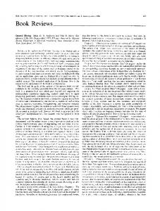
Fig. 2. A comparison of our method to other two particle filters for a linear, Gaussian system. The top row shows the particles and weights obtained for each algorithm. Below the weighted histograms of the samples is compared to the exact Gaussian density. This similarity is measured in the third row with the Kullback-Leibler distance between the real and the estimated distributions for different sample sizes. Observe how our method achieves a lower distance (a higher similarity) even for a few particles.

is kept below a certain threshold ǫ with a probability 1 − δ. Please, refer to [8] for further details. To summarize the introduction of our algorithm we present an algorithmic description of the overall method in Table II. IV. E XPERIMENTAL R ESULTS In this section we will first present simultations for comparing our filtering algorithm to others, and next we will show experiments where our approach is applied to robot localization (position tracking). A. Simulations We have considered here a one-dimensional linear system with Gaussian transition and observation models. Such a simple system allow us to contrast the output of the different filters with the analytical solution from a Kalman filter (KF) which provides us the exact posterior. The situation being simulated is that of an observation model much more peaked than the prior distribution obtained from the system transition model, a situation similar in mobile robotics to a poor motion model (such as odometry) and a very precise sensor (such as a laser scanner). The top graphs of Fig. 2 represent the location and weights of the obtained particles with three different algorithms: a SIR filter with a standard proposal distribution [21], an auxiliary particle filter (APF) [19], and our method. We can observe how the standard proposal leads to most of the particles being wasted in non relevant areas with negligible importance weights. The APF introduces a great improvement in this sense, since particles are more concentrated in the area of interest. However, the weights still contain a certain variance. In contrast, our optimal algorithm generates particles distributed exactly according to the true posterior, thus they all have the same weights. To measure the accuracy of each particle filter we have reconstructed the estimated densities by means of weighted histograms, shown in the middle row of Fig. 2 along with the analytical solution from the KF. To evaluate each algorithm, we have computed the KLD between the analytical and the estimated distributions for a range of sample sizes (we have disabled here the capability of automatically determining the

sample size in our method for comparison purposes with the others). The average KLD for 1000 realizations, shown in the bottom row of Fig. 2, confirms that our approach gives estimations closer to the actual posterior (with less particles) than previous methods. B. Localization The following experiments consist of tracking the pose of a mobile robot equipped with a laser range finder while it is manually guided through an office environment. Concretely, the path and the (already built) map of the environment are shown in Fig. 3(a). The purpose of the first experiment is to compare the accuracy in the localization between our optimal sampling mechanism and the standard proposal distribution. The resolution of the grid is 0.04m, and the non-parametric observation model is the likelihood field described in [23]. The accuracy has been calculated by averaging the localization errors of all the particles at each time step, and using as the ground truth the robot poses estimated while the map was first built. Significant results are obtained by averaging over 100 executions for each sample size. The capability of adapting the sample size in our algorithm has been disabled in this first experiment to provide a fair comparison to a standard PF. The most interesting conclusion from the results, in Fig. 3(b), is that our optimal PF has an excellent performance starting from just one particle (an average error of roughly 0.10m), whereas the standard proposal needs about 10 particles or more to avoid the filter to diverge (e.g. the average error of 6m for one particle means the filter has lost track of the localization). On the other hand, our method requires more computation time than the standard approach. For example, for 100 particles, ours takes 50.56s for the whole experiment while the standard PF takes 9.91s only. Thus, one could argue that a standard PF with more particles would achieve a similar accuracy than our optimal PF for the same computation time. Actually, we can see in the graphs that our method always achieves a better accuracy than the standard approach, even with much fewer particles and a similar computation time.

R EFERENCES

1m

End

Start

Robot path during localization

(a) Average positioning error (meters)

10 Standard proposal PF Our optimal PF 1

0.1

0.01

Number of particles

1

10 (b)

Number of particles

300 (c)

400

100

104 103 102 101 0

100

200

500 Time 600 steps

Fig. 3. Results for localization experiments. (a) The map used for the experiment and the robot path. (b) The average positioning error using the standard proposal and our optimal algorithm, both for different sample sizes (results averaged over 100 repetitions). Observe how our method performs well even for just one particle. (c) The number of particles for our method (determined automatically), starting in a situation of global localization with 10000 particles distributed uniformly.

A second localization experiment has been carried out where the adaptive sample size capability of our algorithm is enabled. In this case, we start in the situation of global localization (initially there are 10000 particles distributed uniformly over the whole environment). As shown in Fig. 3(c), the sample size drastically falls in the first few iterations to the range of 20-30 particles, and it remains approximately fixed along the whole experiment. This is because there are no situations where the sensors become particularly ambiguous. V. C ONCLUSIONS In this paper we have identified a problem, localization with grid maps, where a particle filter is required but the lack of a closed-form observation model prevent the direct application of the optimal proposal distribution. We have derived a new algorithm that allows a particle filter to exploit this optimal proposals even for non-parametrical models. We have shown how the method focuses the samples in the relevant areas of the state space better than previous particle filter algorithms in simulated experiments, as well as the suitability to real robot localization. Additional work will be required to explore the interesting applications of this method to SLAM, where a dynamic number of optimally distributed particles will improve recent works on RBPF-based grid mapping.

[1] M. Arulampalam, S. Maskell, N. Gordon, T. Clapp, D. Sci, T. Organ, and S. Adelaide, “A tutorial on particle filters for online nonlinear/nonGaussianBayesian tracking,” IEEE Transactions on Signal Processing, vol. 50, no. 2, pp. 174–188, 2002. [2] T. Cover and J. Thomas, Elements of information theory. Wiley New York, 1991. [3] A. Davison, I. Reid, N. Molton, and O. Stasse, “MonoSLAM: RealTime Single Camera SLAM,” IEEE Transactions on Pattern Analysis and Machine Intelligence, vol. 29, no. 6, June 2007. [4] M. Dissanayake, P. Newman, S. Clark, H. Durrant-Whyte, and M. Csorba, “A solution to the simultaneous localization and map building (SLAM) problem,” IEEE Transactions on Robotics and Automation, vol. 17, no. 3, pp. 229–241, 2001. [5] A. Doucet, N. de Freitas, and N. Gordon, Sequential Monte Carlo methods in practice. Springer, 2001. [6] A. Doucet, N. de Freitas, K. Murphy, and S. Russell, “RaoBlackwellised particle filtering for dynamic Bayesian networks,” in Proceedings of the Sixteenth Conference on Uncertainty in Artificial Intelligence, 2000, pp. 176–183. [7] A. Doucet, S. Godsill, and C. Andrieu, “On sequential Monte Carlo sampling methods for Bayesian filtering,” Statistics and Computing, vol. 10, no. 3, pp. 197–208, 2000. [8] D. Fox, “Adapting the Sample Size in Particle Filters Through KLDSampling.” International Journal of Robotics Research, vol. 22, no. 12, pp. 985–1003, 2003. [9] D. Fox, W. Burgard, F. Dellaert, and S. Thrun, “Monte Carlo localization: Efficient position estimation for mobile robots,” Proc. of the National Conference on Artificial Intelligence (AAAI), vol. 113, p. 114, 1999. [10] N. Gordon, D. Salmond, and A. Smith, “Novel approach to nonlinear/non-Gaussian Bayesian state estimation,” Radar and Signal Processing, IEEE Proceedings on, vol. 140, no. 2, pp. 107–113, 1993. [11] G. Grisetti, C. Stachniss, and W. Burgard, “Improved Techniques for Grid Mapping With Rao-Blackwellized Particle Filters,” IEEE Transactions on Robotics, vol. 23, pp. 34–46, Feb 2007. [12] S. Julier and J. Uhlmann, “A new extension of the Kalman filter to nonlinear systems,” Int. Symp. Aerospace/Defense Sensing, Simul. and Controls, vol. 3, 1997. [13] R. Kalman, “A new approach to linear filtering and prediction problems,” Journal of Basic Engineering, vol. 82, no. 1, pp. 35–45, 1960. [14] J. Liu and R. Chen, “Sequential Monte Carlo Methods for Dynamic Systems,” Journal of the American Statistical Association, vol. 93, no. 443, pp. 1032–1044, 1998. [15] M. Montemerlo, “FastSLAM: A Factored Solution to the Simultaneous Localization and Mapping Problem With Unknown Data Association,” Ph.D. dissertation, University of Washington, 2003. [16] M. Montemerlo, S. Thrun, D. Koller, and B. Wegbreit, “FastSLAM: A factored solution to the simultaneous localization and mapping problem,” Proceedings of the AAAI National Conference on Artificial Intelligence, pp. 593–598, 2002. [17] H. Moravec and A. Elfes, “High resolution maps from wide angle sonar,” in Proceedings of the IEEE International Conference on Robotics and Automation, vol. 2, 1985. [18] K. Murphy, “Bayesian map learning in dynamic environments,” Advances in Neural Information Processing Systems (NIPS), vol. 12, pp. 1015–1021, 1999. [19] M. Pitt and N. Shephard, “Filtering Via Simulation: Auxiliary Particle Filters.” Journal of the American Statistical Association, vol. 94, no. 446, pp. 590–591, 1999. [20] D. Rubin, “A noniterative sampling/importance resampling alternative to the data augmentation algorithm for creating a few imputations when fractions of missing information are modest: The SIR algorithm,” Journal of the American Statistical Association, vol. 82, no. 398, pp. 543–546, 1987. [21] ——, “Using the SIR algorithm to simulate posterior distributions,” Bayesian Statistics, vol. 3, pp. 395–402, 1988. [22] S. Thrun, Robotic Mapping: A Survey. School of Computer Science, Carnegie Mellon University, 2002. [23] S. Thrun, W. Burgard, and D. Fox, Probabilistic Robotics. The MIT Press, September 2005. [24] E. Wan and R. Van Der Merwe, “The unscented Kalman filter for nonlinear estimation,” in Proceedings of the IEEE Adaptive Systems for Signal Processing, Communications, and Control Symposium, 2000, pp. 153–158.