and open-loop voluntary movement - Semantic Scholar
Recommend Documents
Left SMC (4). â28 â38. 52. 7.02. The x, y, and z coordinates refer to position within the stereotactic space according to the atlas of Talairach and Tournoux (1988) ...
scan session. Assessment included Scales for the Assessment of Positive and Negative Symptoms (Andreasen, 1983, 1984),. Barnes Akathisia Scale (Barnes, ...
Lia Kvavilashvili. School of Psychology .... highly active recent memories, as suggested by Conway (2005). Initial evidence .... 7=high). The mean ratings as a function of cue type (involuntary, voluntary) and cue valence. (negative, neutral ...
tional dislocation of his right shoulder (fig 1a, b). All the movements were painless and perhaps enjoyable. The examination of the shoulder after the voluntary ...
tenable for other Korean/Japanese NPIs, it cannot be extended to the. Japanese NPI "sika". ... Dare-mo Mary-o mi-nakat-ta. Anybody Mary-Acc .... way to [Spec,TP], subject NPIs move through [Spec,NegP] to get licensed by Neg as shown in ...
about regulations: A case study of in the Missouri Ozarks. Society Nat. Resources ... New York: Oxford=World Bank. Wheeler, D. 2001. Racing to the bottom?
Jul 27, 2017 - several cultural tasks to investigate Shenzhen, known as China's ongoing âSouth ... of Shenzhen scored higher than China inland residents in ...
Arthur Sherwood. AbstractâIn this paper, a method for ... sEMG was recorded bilaterally from quadriceps, adductor, ham- string, tibialis anterior, and triceps ...
Aaron Schurger 1,2,3,5,6, Nathan Faivre1,3,4, Leila Cammoun1,3, Bianca Trovó5,6 ..... Lopresti-Goodman, S. M., Richardson, M. J., Silva, P. L. & Schmidt, R. C. ...
Mar 17, 2013 - Formal thought disorder, the type-token ratio and disturbed. References .... as simple length inmaw, Maat studies have u d the mean wgmentai ...
of arm-raising movement was mainly local, that is to say at the level of trunk and .... agoinst and antagonist muscles expressed in terms of .... anatomical limit.
Why Breed? Like the Greek ... calling. is noble free choice. bf achieved without
breeding. Many children wait for ... apparent, but his ideas linger strong. Women
s ...
The activation function for this model is a linear function of ... function does not vary, but the movement trigger threshold varies across trials in a Gaussian fashion ...
Mar 31, 2014 - The Lokomat® (Hocoma AG, Volketswill, Switzerland), a driven-gait orthosis (DGO) device attached to a tread- mill with BWS, was developed ...
the recent development of more accurate and relatively cheap wireless/wearable .... The phase shift registration alters the time domain by δj for each waveform x ...
Rowena B. Valencia-Gica, Russell S. Yost, Guy S. Porter, and Rosalin Pattnaik. Abstract: ...... Mclaughlin, M. R., K. R. Sistani, T. E. Fairbrother, D. E Rowe. 2005.
marker placed on the anterior superior iliac spine. Statistical methods. A paired Student t test was used to compare side steps to the right and side steps to the ...
add-on for the Xbox 360 video console, which enables user interaction through movements and ... interaction could greatly benefit existing data-driven (e.g., computer vision) approaches ..... PhD thesis, Technical University of. Crete. (2009).
Oct 17, 2016 - Stress-Related Growth Scale (SRGS), Clinician-Administered PTSD Scale (CAPS), and Connor-Davidson Resilience Scale. (CD-RISC) were ...
Jul 4, 2005 - Toward the next generation. ... Development is a classic focus of Vygotskian cultural-historical ..... the
that simulates the time-varying changes of the vocal tract and acoustic wave propagation. ..... simulation of the phrase âHappy Birthdayâ is shown in Figure 4.
Jul 4, 2005 - âConsider, for example, the structure of medical knowledge in a common family practice type setting, whi
function is to regulate neural signals in other parts of the brain. Most is known about its regulatory actions on neurons that control movement and posture.
Dec 20, 2016 - Craig A. A new view of pain as a homeostatic emotion. Trends .... Turk DC, Dworkin RH, Allen RR, Bellamy N, Brandenburg N, Carr DB, et al.
and open-loop voluntary movement - Semantic Scholar
School of Medicine, University of Otago, Christchurch 8001, New Zealand. (e-mail: ..... of the change in signal location is formed online using adaptive linear FIR filters. In ... This tech- nique cannot be employed in a nonlinear generalization as a nonlinear ..... Laboratories of the I.T.T., Harlow, Essex, U.K., and started 40 ...
1242
IEEE TRANSACTIONS ON BIOMEDICAL ENGINEERING, VOL. 49, NO. 11, NOVEMBER 2002
Simulating Closed- and Open-Loop Voluntary Movement: A Nonlinear Control-Systems Approach Paul R. Davidson, Member, IEEE, Richard D. Jones*, Senior Member, IEEE, John H. Andreae, Senior Member, IEEE, and Harsha R. Sirisena, Member, IEEE
Abstract—In many recent human motor control models, including feedback-error learning and adaptive model theory (AMT), feedback control is used to correct errors while an inverse model is simultaneously tuned to provide accurate feedforward control. This popular and appealing hypothesis, based on a combination of psychophysical observations and engineering considerations, predicts that once the tuning of the inverse model is complete the role of feedback control is limited to the correction of disturbances. This hypothesis was tested by looking at the open-loop behavior of the human motor system during adaptation. An experiment was carried out involving 20 normal adult subjects who learned a novel visuomotor relationship on a pursuit tracking task with a steering wheel for input. During learning, the response cursor was periodically blanked, removing all feedback about the external system (i.e., about the relationship between hand motion and response cursor motion). Open-loop behavior was not consistent with a progressive transfer from closed- to open-loop control. Our recently developed computational model of the brain—a novel nonlinear implementation of AMT—was able to reproduce the observed closed- and open-loop results. In contrast, other control-systems models exhibited only minimal feedback control following adaptation, leading to incorrect open-loop behavior. This is because our model continues to use feedback to control slow movements after adaptation is complete. This behavior enhances the internal stability of the inverse model. In summary, our computational model is currently the only motor control model able to accurately simulate the closed- and open-loop characteristics of the experimental response trajectories. Index Terms—Adaptive inverse control, internal models, motor control modeling, motor learning, tracking task.
I. INTRODUCTION
W
HEN controlling voluntary movement the human central nervous system (CNS) acts as a hybrid feedforward/feedback adaptive control system. Multimodal sensory information is employed at several levels in the motor hierarchy
Manuscript received September 16, 2001; revised June 3, 2002. Asterisk indicates corresponding author. P. R. Davidson is with the Department of Electrical and Electronic Engineering, University of Canterbury, Christchurch, New Zealand, and the Department of Medical Physics and Bioengineering, Christchurch Hospital, Christchurch 8001, New Zealand. *R. D. Jones is with the Department of Electrical and Electronic Engineering, University of Canterbury, Christchurch, New Zealand, the Department Medical Physics and Bioengineering, Christchurch Hospital, Private Bag 4710, Christchurch 8001, New Zealand. He is also with Medicine, Christchurch School of Medicine, University of Otago, Christchurch 8001, New Zealand (e-mail: [email protected]). J. H. Andreae and H. R. Sirisena are with the Department of Electrical and Electronic Engineering, University of Canterbury, Christchurch 8001, New Zealand. Digital Object Identifier 10.1109/TBME.2002.804601
to modify outgoing motor commands, resulting in feedback or closed-loop control [1]. Feedforward or open-loop mechanisms are also employed extensively, particularly for the execution of fast movements where feedback propagates too slowly to affect the motor response [2]. The influential feedback-error learning (FEL) [3] model suggests that multiple feedback controllers exist at the spinal, brainstem and cerebral levels which operate in parallel with feedforward pathways containing adaptive inverse models. In adaptive model theory (AMT) [4] feedback and feedforward influences are combined in series [5]. In these and other similar models, feedback control is used to correct errors while an inverse model is simultaneously tuned on-line for accurate feedforward control. Thus, both models predict that after extensive practice at a motor task, once an accurate inverse model has been acquired, the role of the feedback pathways is limited to the correction of disturbances. If feedback of a motor task is withheld then performance should remain unaffected, except for random drift caused by noise. This is because in the absence of feedback, and after extensive practice, both models rely exclusively on their inverse models to generate the motor command. We have developed a novel nonlinear implementation of AMT which offers an alternative prediction. Our implementation is able to simulate the human capacity to control nonlinear dynamic systems like the musculoskeletal system. In contrast with other AMT implementations and with FEL, our model predicts that the feedback pathways remain active and play a central role in generating the primary motor command, even after extensive training at a motor task. AMT suggests that the CNS forms an accurate nonlinear forward model which is then inverted in some fashion. In our implementation, the forward model is subsequently inverted by placing it in an internal feedback loop [6]. This method is parsimonious as it requires few additional parameters over those required to form the forward model. In principle, the loop gain needs to be very high to generate an accurate inverse of the forward model but the loop and, hence, the inverse, become increasingly unstable as the feedback gain is increased. Hence, an approximate inverse is generated by lowering the gain of the internal feedback loop used for inversion. For optimum overall performance, inaccuracies in the inverse are restricted to low frequencies, allowing the feedback pathways to contribute usefully. This is achieved by adding derivative and integral components to the loop gain. The closed-loop behavior of our model is, therefore, very similar to existing models but its open-loop behavior is substantially different. Our model predicts that open-loop tracking is inaccurate at low frequencies and progressively more accurate at higher
DAVIDSON et al.: SIMULATING CLOSED- AND OPEN-LOOP VOLUNTARY MOVEMENT: A NONLINEAR CONTROL-SYSTEMS APPROACH
frequencies. Other AMT implementations and FEL predict that open-loop behavior, once any random drift effects have been eliminated, is particularly accurate at low frequencies. An experimental study, looking at human manual tracking behavior under both closed- and open-loop conditions, has previously been published [7]. Here, we re-evaluate the data from this study to test whether the open-loop tracking behavior, the key observable difference between our model and other motor control models, is observed in human behavior. We also introduce our implementation of AMT in additional detail. The study data shows that human open-loop tracking late in learning exhibits high-pass amplitude characteristics and is particularly inaccurate at low frequencies, in agreement with the predictions of our model. This suggests that the feedforward pathways of the motor system might employ an approximate inverse model like that used in our simulation.
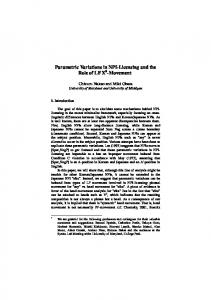
II. HUMAN TRACKING STUDY Twenty human subjects (13 male and 7 female) were trained on 1-D pursuit tracking task using steering wheel for input and a computer monitor for visual feedback. Rotation of the wheel moved an arrow horizontally on the screen and subjects were required to follow a target moving vertically down the screen. Full response feedback was provided for the initial interval of each tracking run, during which subjects partially learned to control a novel visuomotor relationship. Feedback was then removed by blanking the response arrow. This training and blanking cycle was repeated several times until no further closed-loop performance improvement was evident. Response trajectories were recorded at 60 Hz, thereby providing a record of closed- and open-loop tracking behavior at discrete intervals during the adaptation process. This was repeated for two different visuomotor relationships (static nonlinear and dynamic linear). The screen setup is shown in Fig. 1. The experiment comprised 25 consecutive 103-s tracking runs separated by rests of 20-s duration. For each run the subject was asked to “keep the point of the arrow on the line as accurately as possible.” The subject was then told that the arrow would disappear late in the run and that they were required to continue the task by estimating the position of the arrow. All subjects were initially asked to control a simple zeroorder external system (i.e., wheel angle proportional to response pointer position). These practice sessions were to allow subjects to learn as much about the target and tracking system as possible. This facilitates the assumption that only the external system was learned in the following runs. Ten runs of the zeroorder task were performed, after which learning plateaued. At this point the stochastic characteristics of the target signal, the kinematic and dynamic properties of the steering wheel, and the wheel-to-display relationship are considered to have been maximally learned. The subjects were then asked to control a new visuomotor relationship, implemented by altering the characteristics of the external system. Subjects were split into two groups, labeled A and B. Both groups were required to train on their new external system for 15 runs. This duration was selected to be long enough
1243
Fig. 1. Preview random tracking task. Subject alters horizontal position of arrow to keep point on descending target waveform. Arrow moves along horizontal line. The small box at intersection of line and target emphasizes the current target position.
to characterize any learning trend but not so long as to introduce noticeable fatigue. Group A controlled a linear dynamic system. The dynamics were produced by passing the motor response through an infinite impulse response (IIR) filter: a third-order Chebyshev Type I low-pass filter with cutoff frequency of 3 Hz. Group B was required to learn a static nonlinear system. The system was a cubic function of input angle, scaled to provide a challenging variation in gain while remaining controllable. The function was displaced from center to increase the difficulty of the task by avoiding symmetry. The function used was (1) where is the steering wheel angle in degrees (centered at 90 ) and is the target position relative to the left edge of the screen (millimeters). The target signal comprised two consecutive sections as follows: 1) Unblanked Training Signal: 68 s of a pseudorandom waveform generated from superposition of 50 sinusoids of equal amplitude and equally spaced in frequency with random phase from 0.007 Hz up to 0.6 Hz, 75% full scale deflection. 2) Blanked Assessment Signal: Identical to the first 28 s of the training signal except for removal of feedback to the subject by turning off the response arrow. The two sections were combined and separated by a 7-s interval where the target returned to the center of the screen. All three sections combined to form a single continuous 103-s target signal, which was used for all runs in the experiment. The subject was also presented with an 8-s preview of the target to improve prediction of the target signal. III. MODEL STRUCTURE In AMT, the brain is considered to operate continuously to translate an intermittently planned trajectory of desired sensory consequences into smooth coordinated movements. This sensorimotor transformation is achieved by passing the desired trajectory through a series of inverse models implemented as adaptive
1244
IEEE TRANSACTIONS ON BIOMEDICAL ENGINEERING, VOL. 49, NO. 11, NOVEMBER 2002
Fig. 2. Simulation structure. Open-loop tracking achieved by moving switch to upper-most position. T is the target signal, R3 is the desired trajectory, MR is ^ is the predicted response. OTG is an intermittent optimum trajectory generator (see [12]). the motor response, R is sensory feedback of the actual response and R Afferent and efferent delays, representing lumped transmission and processing delays respectively, are partially compensated for by forward model observer P and target predictor T P .
neural filters. The adaptive filters control the appropriate timing and amplitude of muscle output. Neilson et al. [4] proposed that the overall inverse model is physically realized in the form of three serially cascaded multiple-input multiple-output nonlinear dynamic inverse models. These models are inverse representations of three levels of the human plant—the muscle control system (MCS), the biomechanical system (BM), and the external system (E). These three subdivisions are delineated by the four levels of continuously available sensory feedback in the human motor system: efference copy of outgoing motor commands, tension feedback from Golgi tendon organs, joint angle information from various modalities including kinesthesia and vision and, finally, multimodal feedback on the sensory consequences of the movement. For convenience the resulting inverse models are termed MCS , BM (which together compose an inverse dynamics model) and E (the inverse kinematics model). In a previous implementation of AMT [4], linear adaptive finite impulse response (FIR) filters were employed to mimic the formation of the nonlinear internal models thought to exist in the brain. One of the principal advantages of forming a linear model is that the corresponding inverse model can be determined analytically from the parameters of the forward model. taps can be expressed For example, a linear FIR filter with where is the filter output, as is the filter input, and is the th filter tap weighting. given The inverse of this filter, that is a filter generating , can be calculated by simply rearranging to give . Unfortunately this initial linear implementation of AMT, while powerful in its ability to predict motor behavior, is incomplete because the human CNS is required to control nonlinear dynamic systems. The human musculoskeletal system exhibits complex and highly nonlinear dynamics [8], [9] which a linear filter model cannot capture. Additionally, the successful control of nonlinear dynamic mechanical systems, such as bicycles, motor vehicles, and jet aircraft, is known to be within the normal range of human ability. The same simple analytical
relationship between the forward and inverse model is not, in general, available when the forward model is represented in a nonlinear adaptive filter. The accurate online formation of an inverse model of a nonlinear system from input and output data is a difficult problem. There have been numerous efforts to find a robust neurobiologically plausible solution [3], [10], [11], [13]. The primary distinction between our model and the linear implementationof AMTisthat thelinearadaptivefiltersarereplaced with adaptive nonlinear dynamic filters. This necessitates the selection of an appropriate filter structure which maintains the online adaptive performance of AMT while capturing the nonlinear learning capacity of the CNS. Since the change to nonlinear filters invalidates the analytic inversion process used to form an inverse model from a forward model, the structure of the AMT model requires additional alteration. Our model includes circuitry to approximate the inverse of the forward model and, consequently, must also include circuitry to compensate for any errors in the resulting inverse by using the actual motor command and the forward model to generate a prediction of the actual response. A. Overall Structure The structure of the new model is shown in Fig. 2. Like other AMT implementations, our model includes a feedback controller called an optimum trajectory generator (OTG). The OTG implements receding-horizon optimal control by intermittently issuing optimum corrective movements based on stochastic prediction of the target and response trajectories (see [12]). The OTG parameters used here were set to typical values as determined experimentally by Sriharan [13]. The overall simulation operated at a discrete sampling rate of 20 Hz in accordance with the AMT model [4]. The efferent delay represents the time between the generation of a motor command in the brain and the first measurable force in the 50 ms in the simulation. The muscles. This was set to afferent delay, representing the remaining loop delay (including 100 ms. The delay visual processing time), was set to
DAVIDSON et al.: SIMULATING CLOSED- AND OPEN-LOOP VOLUNTARY MOVEMENT: A NONLINEAR CONTROL-SYSTEMS APPROACH
Fig. 3. Forward model observer structure. The response input can be used for state estimation allowing more accurate response prediction. (afferent) delay and is the outgoing (efferent) delay.
values were quantized in accordance with the 50-ms sampling period of the simulation and are within the normal range quoted in the literature [14], [15].
1245
is the incoming
state of the plant. In our model, the forward model observer expresses the controlled system as a function of its input signal, the motor response , and the previous sample of the response signal
B. Nonlinear Dynamic Filters Locally recurrent neural networks (LRNNs) act as adaptive filters in our nonlinear AMT implementation. LRNNs are capable of dynamically trading off representation of temporal depth for memory resolution [16] which means that the temporal features of the problem at hand do not need to be known a priori. It is worth noting that the LRNN filters could be substituted by more realistic models of the cerebellum [17] or basal ganglia [18] as they become available. The LRNN structure used in simulation employs neurons with somatic, as opposed to synaptic, adaptive IIR dynamics [19]. The neurons employ sigmoidal activation functions, mimicking the expected activation for a functional group of biological neurons having a Gaussian distribution of activation thresholds [20]. These neurons were formed into a three-layer fully connected neural network. A gradient descent adaptation algorithm was developed, using dynamic back-propagation techniques as suggested by Back and Tsoi [21], to train the resulting network. To maintain an acceptable on-line learning rate, an adaptive linear circuit is maintained in parallel with this nonlinear structure. In the simulations presented here, each LRNN consisted of 16 neurons with adaptive second-order dynamics in the hidden layer and a single-output neuron with a linear threshold. There were one or two inputs to each network depending on its function in the model (there were two inputs in the case of the forward model observer). The parallel adaptive linear filter had a buffer depth of 3 s. C. Adaptive Forward Modeling Our model employs a nonlinear forward-model observer which represents the controlled system as a (FMO) function not only of its current input signal, as in the linear AMT implementation, but also as a function of its previous output signals. Thus, observer models include an additional input which can be seen as providing an estimate of the current
(2) where is the simulation step size. The required structure for the implementation of a forward model observer within our AMT implementation is shown in Fig. 3. In practice, all that is required is the addition of a second input to the forward model for the delayed response signal, which can be seen as a state estimation input. The LRNN previously described is provided with an additional input for the delayed sensory response signal. Hence, becomes a nonlinear dynamic multiple-input single-output function. D. Adaptive Stochastic Prediction AMT hypothesizes that the stochastic properties of the target and disturbance signals are modeled adaptively in neural circuitry so that an optimum prediction of the future values might be generated [5], [22]–[24]. In the linear implementation, a moving-average stochastic model of the change in signal location is formed online using adaptive linear FIR filters. In our implementation, this idea is generalized and an adaptive nonlinear filter is employed to model the stochastic properties of the signal. The predictor structure is also extended to include an autoregressive component for added generality [25]. The resulting predictor structure is a nonlinear moving-average auto-regressive (NARMA) predictor. In moving to a nonlinear predictor, it becomes impossible to model the change in signal location by differentiating, as in other implementations, because a nonlinear model requires absolute position information. Conversely, moving to a model based entirely on absolute position was found to produce unacceptable performance [26]. This difficulty was solved by dividing the predictor into parallel linear and nonlinear channels and providing these with differential and absolute inputs respectively. The outputs of the parallel channels are added together and the error signals adjusted accordingly.
1246
IEEE TRANSACTIONS ON BIOMEDICAL ENGINEERING, VOL. 49, NO. 11, NOVEMBER 2002
Fig. 4. Circuitry for forming a NARMA stochastic one-step predictor. The circuitry uses a novel combined parallel differential-linear and absolute-nonlinear structure.
A general NARMA model for a stochastic signal can be expressed as a Gaussian noise input
given
(3) only the term is unknown. We make At time . Since has zero the assumption that mean this is true whenever is an odd function, in which case at time is simply the optimum prediction of
(4) The resulting network exhibits improved performance in predicting nonlinear stochastic signals without any degradation in performance for predicting linear signals [26]. The complete network for the one-step NARMA predictor used in the model is shown in Fig. 4. E. Adaptive Disturbance Compensation In AMT, the disturbance signal is modeled as a stochastic process added to the output of a deterministic plant. This allows the disturbance component of the afferent information to be identified by subtracting the estimated reafference, generated by the forward model, from the actual afference. The resulting disturbance signal is called the exafference, that part of the sensory feedback “generated by external inputs.” The future exafference is then predicted using the stochastic methods mentioned in Section III-D. The use of a FMO effectively alters the definition of exafference in our implementation. Exafference now becomes that part of the response signal which is unpredictable given the current state of the plant. The predictable component, which previously remained part of the exafference, must now be compensated for and this is achieved by the adaptive response predictor. The disturbance compensation structure is included in Fig. 2.
F. Adaptive Response Prediction In previous implementations of AMT, the only adaptive feedback control element is the stochastic disturbance predictor [24]. Response prediction, employed by the OTG for planning response trajectories, is based on previously planned responses. Since, in the case of linear AMT, the inverse model is the exact inverse of the forward model there is nothing to be gained by passing the motor response through the forward model. This resulting signal is simply the desired response produced by the OTG. Consequently, the response prediction system in linear implementations of AMT is not an adaptive process. In a nonlinear implementation, however, the inverse model is, in general, only an approximate inverse of the function defined in the forward model. Hence, the output of the forward model constitutes a more accurate estimate of the actual response than the desired response. This information must be provided to the OTG for use in trajectory planning. Assuming a forward model observer is available, a predictive cascade [9] of these models can be formed to generate the reto in steps of sponse predictions from size in time. These accurate predictions can then be used by the OTG in planning future sub-movements. The predictive cas, cade of forward models is suitable for predictions up to up to which time motor response information is available. For predictions beyond this, up to one planning time period ahead , the existing method based on the preplanned desired of response is used for prediction. G. Nonlinear Inversion In the linear AMT implementation, the forward model is inverted analytically to generate an inverse model. This technique cannot be employed in a nonlinear generalization as a nonlinear mapping cannot, in general, be inverted analytically. The inverse must be estimated using function approximation techniques. The feedback-error learning [27] scheme elegantly solves this problem, forming an inverse model directly without the necessity for a forward model, however, the same scheme cannot be employed within the AMT architecture [26]. Jordan’s forward and inverse modeling scheme [10] also solves
DAVIDSON et al.: SIMULATING CLOSED- AND OPEN-LOOP VOLUNTARY MOVEMENT: A NONLINEAR CONTROL-SYSTEMS APPROACH
Fig. 5. Proposed nonlinear inversion scheme. The feedback gain proportional, integral and differential components.
K includes
the problem, but in a relatively unrealistic fashion requiring backpropagation through a forward model. The problem is addressed in our implementation by embedding the forward model in an internal feedback loop, as first suggested by Miall et al. [6]. However, the high-gain feedback loop approach advocated by Miall was found to be unstable under typical simulated conditions. Consequently, a relatively low loop-gain as specified by (5) where , , and are adjustable gain parameters and is the feedback loop error, was employed to enhance the stability of the loop (see Fig. 5). No other use of a PID gain to improve the stability of an internal feedback loop was found in the literature. This approach effectively trades the accuracy of the inverse for internal feedback loop stability. The performance of the overall system was found to remain acceptable due to the presence of feedback introduced in the trajectory planning circuitry. Since this technique only requires the storage of a forward model for each system, instead of both a forward model and an inverse model, the approach is more parsimonious than less direct methods (see, e.g., [10]). In simulation, the choice of gain of the feedback loop used for inversion of the forward model had a strong impact on behavior. In the work presented here, it was assumed that the loop gain was constant during the simulation. A small integral component was necessary to eliminate steady-state error in the in0.05 was used for all runs and verse model. Consequently, is not explicitly quoted in the following results where loop gain and were tuned manually to parameters are mentioned. achieve optimum performance. IV. SIMULATION A full simulation of the experiment described in Section II was carried out using our AMT implementation. Response cursor blanking was simulated by removing response feedback from the tracking simulation. Losing response feedback could reasonably be expected to cause the controller to stop making corrective movements. This implies the complete disengagement of the feedback control pathways. In the model, this
1247
can be achieved by replacing the predicted response with the desired response (see Fig. 2). Because the error between desired and actual response observed by the OTG becomes zero no corrective movements are executed. Note that the OTG continues planning optimum trajectories but based only on target signal predictions. Adaptation was also halted during blanking to prevent catastrophic unlearning. Noise was modeled in closed- and open-loop by adding bandlimited Gaussian white noise to the motor response . The variance of the Gaussian white noise generator was set to zero for noise-free simulations. Noise was added to both the differential and absolute pathways of the model. When the differential pathways are integrated this results in some random drift at the output as observed experimentally. A. Initial Parameters The practice runs were simulated with the target predictor and internal model parameters initialized to small random values. The parameters reached after ten simulated runs in control of the zero-order practice system were then used in the ensuing simulations. This ensured that the simulator was in approximately the same state as the experimental subjects at the beginning of the experimental runs. In the experimental design, care was taken to eliminate targettrajectory prediction as a confounding source of learning. Consequently, the target predictor was assumed to have been accurately tuned from the beginning of the simulation of the experto , imental runs. The predicted values where is the prediction depth, were set to their exact values. B. Simulation Procedure The simulation began with ten practice runs as performed in the experimental study. In these a simple zero-order gain was assigned as the external system. The adaptation coefficient of the forward model was set to 0.0015 which was found, by trial and error, to approximate the learning rate observed during the experimental practice. It was important that be set so that learning had essentially plateaued after the final (tenth) run. The 10 to provide acinternal feedback loop-gain was set to ceptable inverse model performance during the initial learning process. This arbitrary value was acceptable since the loop-gain has relatively little effect on the learning of the forward model (an assertion confirmed by adjusting and comparing forward model characteristics). The model weights at the end of the ten practice runs were stored for use in the subsequent experimental runs. The simulated practice results could not be compared directly with the experimental results until after the internal model had approximately converged, which was shown to be by about run five [7]. This is because human subjects are likely to begin the practice runs using an approximate internal model based on past experience, whereas the model was simply initialized with random weights. It was necessary to determine appropriate values for the loop-gain and adaptation rate parameters prior to the full experimental run simulations. Once the practice run learning was complete, the forward model itself was affected only minimally by variation in loop-gain and adaptation rate (provided stability
1248
IEEE TRANSACTIONS ON BIOMEDICAL ENGINEERING, VOL. 49, NO. 11, NOVEMBER 2002
Fig. 6. Simulated RMS error in relation to experimental results (final run). Experimental results indicated with solid lines, simulated results indicated with crosses. Bars indicate experimental standard deviation.
was maintained). This allowed a strategy to be devised whereby appropriate parameters for the experimental runs could be determined a priori. The previously learned zero-order forward model was loaded into the simulation, with adaptation turned off, and iterative alterations to the parameters were made so that their effect on closed- and open-loop trajectories could be judged efficiently. It was hoped that a single set of parameters could be found that would perform acceptably across all conditions in the experiment. The same experimental procedure and model parameters were used for the dynamic linear and static nonlinear external systems. Simulation of the experimental runs began with the dynamic linear external system. Fifteen runs were simulated in accordance with the 15 experimental runs performed by the human subjects. The model was initialized with several different adaptation coefficients so that an appropriate learning 0.0015 produced a response with rate could be determined. an appropriate closed-loop learning time constant (compared with experimental results from human subjects) and these results are reported. The internal loop-gain settings found to produce good results for a zero-order system was used for these runs. Trial runs with various other feedback-loop gains produced no clear improvements. V. RESULTS A. Experimental Data A graphical summary of the experimental results is included in all simulation result diagrams. The mean and standard deviation of the final experimental run are shown on each diagram.
By using only the final run, instead of the mean across all runs, learning effects do not interfere with the interpretation of results. Thus, the experimental results shown in the diagrams represent the optimum transfer function learned by the subjects. The results from one subject in the static nonlinear group were removed from the analysis due to the open-loop gain of this subject being twice that of any other subject. 1) Learning Trends: Clear learning trends were evident in the closed-loop results for all external systems but the corresponding open-loop learning trends were relatively weak (see Fig. 6). No learning was detected for the dynamic linear external system in open-loop. Learning trends were, however, detected in the open-loop results for both the static nonlinear external system and the practice runs [7]. The discrepancy between closed- and open-loop learning trends may be due to a very large learning rate differential between the feedforward and feedback adaptive controllers, suggesting that very little open-loop learning occurred over the 15 experimental runs. Alternatively there may be another effect obscuring underlying improvement in feedforward performance. Simulation of the learning process aimed to resolve this issue. 2) Transfer Functions: The human tracking experiment produced response trajectories exhibiting unusual open-loop characteristics. There was little evidence of a direct relationship between closed- and open-loop trajectories as predicted by other motor models. The open-loop responses for all external systems showed a mean high-pass gain with a cutoff frequency of approximately 0.3 Hz. The mean gains from 0–0.3 Hz were remarkably similar across all three external systems in the experiment. There was
DAVIDSON et al.: SIMULATING CLOSED- AND OPEN-LOOP VOLUNTARY MOVEMENT: A NONLINEAR CONTROL-SYSTEMS APPROACH
a tendency for phase lead when controlling the two static systems (zero-order and nonlinear). The dynamic linear system exhibited a very large intersubject variability in open-loop phase response, and while the mean exhibits a phase lag, many individuals actually lead the target. Open-loop results for all systems also exhibited a characteristic drop in coherence at low-frequency. Intersubject variance was markedly greater in open-loop tracking compared with closed-loop tracking. The open-loop results do not indicate that the human subjects were attempting to reach a transfer function of unity, representing accurate tracking (as observed for closed-loop tracking). In fact, a quite different relationship between target and response appears to have emerged. This relationship needs to be explained and reproduced in simulation. In contrast with the open-loop results, the closed-loop gain was close to unity across the target bandwidth, as expected for the human operator after extensive training. No attenuation of low frequencies, as observed for the open-loop data, was evident. The gain for the dynamic linear system was higher than the other systems (possibly in compensation for the phase lag introduced by this external system). The mean phase responses were close to zero, except for the dynamic linear system which exhibited uncompensated phase lag. The mean closed-loop coherence was very close to unity for all three systems, indicating relatively little noise or nonlinearity in the response. In general, closed-loop performance at lower frequencies was superior to that at higher frequencies. The closed-loop results indicate that, to varying degrees for all three systems, the human subjects were attempting to reach a transfer function of unity (which represents perfect tracking). B. Simulations Results 1) Parameters: The internal feedback loop parameters were tuned manually to provide a suitable fit. It was noted that a high-frequency gain drop-off was evident even for very high 100). This indicates that the forward model, loop-gains ( as formed during simulation of the practice runs, was not completely accurate. A similar, though much weaker, reduction in high-frequency gain was evident in the experimental results. This effect, however, remains a point of difference between the simulated and experimental results at high frequencies. The parameters found to best match the practice run data were 0.5, 1, and 0.05. Noise, with variances between 0 and 50, was systematically added to the simulation using these 5 generated similar results to parameters. Noise variance the experimental data for the zero-order system. This noise level was used in all following simulations. With the exception of the high-frequency behavior, as explained previously, these parameters produce results similar to the observed experimental results. 2) Dynamic Linear External System: The root-mean-square (RMS) error results for the dynamic linear system are shown in Fig. 6. Removing response feedback caused the RMS error to increase and resulted in a perturbed response trajectory which was consistent with the experimental results. Also, in common with the experimental results, the open-loop RMS error did not improve in proportion with the closed-loop RMS error, remaining at a much higher level (around 35 mm).
1249
Fig. 7. Simulated gain, phase and coherence in relation to experimental results (final run). Experimental results indicated with solid lines, simulated results indicated with crosses. Bars indicate experimental standard deviation.
The transfer function and coherence plots for the final run (number 15) are shown in Fig. 7. The closed-loop results show a phase lag and a gain above 0.9 at all frequencies. The coherence is also very high in closed-loop. These closed-loop results show better performance than the open-loop results due to the action of the feedback controller. The most notable difference between the experimental and simulated transfer functions is the absence in the simulated results of a peak at 0.3 Hz. The cause of this peak in the experimental results is unknown, although it should be noted that the peak was not present in the results of all subjects. The open-loop results show the same characteristic drop in gain and coherence below 0.3 Hz that was observed in the experimental results. The open-loop results also show a gain which, while lower than the mean [approximately one standard deviation (sd) below average], was consistent with the results for several individual subjects. Similarly, the phase response shows a lead with respect to the mean but is consistent with several individuals. By the final run the simulated open-loop trajectory exhibits characteristics which are visually similar to the mean response trajectories of the experimental subjects (see Fig. 8). The simulated trajectory remains within 1 sd of the mean experimental response, so the trajectory shown here could quite conceivably represent a typical human response. 3) Static Nonlinear External System: The closed-loop RMS error results in Fig. 6 show a similar learning trend to the experimental results. The simulated RMS error remains approximately 1 sd higher than the mean experimental results. Notably, the open-loop RMS error results show less learning
1250
Fig. 8.
IEEE TRANSACTIONS ON BIOMEDICAL ENGINEERING, VOL. 49, NO. 11, NOVEMBER 2002
Simulated open-loop response in relation to the target after 15 runs.
than observed experimentally but the increased RMS error and disproportionate learning rate relative to the closed-loop results are reproduced. It was possible to reproduce the weak open-loop learning trend by adjusting the internal feedback loop gain slightly, at the expense of reducing the closed-loop learning rate. Given that no change has been made in the internal loop-gain between this simulation run and the dynamic linear system, the results are acceptably consistent with the mean experimental results. The transfer function and coherence plots for the final run (number 15) are shown in Fig. 7. In closed-loop, the simulated gain below 0.5 Hz was higher than the mean experimental result. The phase response was close to the experimental mean, and the simulated coherence exhibited a characteristic drop above 0.4 Hz as seen experimentally. In open-loop, the gain was again around 1 sd below the mean. Importantly, the open-loop results show the same drop in gain and coherence below 0.3 Hz as was characteristic of the mean experimental results. Fig. 8 shows the simulated open-loop response trajectory for run 15. The response shows similar characteristics to the unusual response trajectories observed in the experiment. The simulated trajectory again remains primarily within 1 sd of the mean experimental response and the trajectory shown here could easily represent a typical human response, though with a relatively low open-loop gain. VI. DISCUSSION Our novel nonlinear implementation of AMT succeeded in generating responses reproducing many of the principal characteristics of the response trajectories obtained during the ex-
perimental study. Importantly, the simulated closed-loop results showed clear evidence of convergence to the target signal by the end of task while the open-loop results did not. This is because, unlike other models, our model continues to employ feedback to control slow movements after adaptation. The inverse model remains inaccurate, particularly at low frequencies, to maximize stability. This is in agreement with the experimental results and contrasts with other AMT implementations and FEL in which the open-loop trajectory converges to the target signal. These results were obtained using a single set of parameters across the range of conditions studied in the experiment (i.e., both closedand open-loop control and several different external systems). It proved possible to generate a high-pass gain with a phase lead in the absence of response feedback while retaining acceptably accurate performance in closed-loop (see Fig. 7). This was possible because the inversion method employed an internal feedback loop, which argues in favor of the existence of similar circuitry in the CNS. The internal loop-gain found to optimally reproduce the experimental results was low ( 0.5, 1, 0.05). It is notable that both FEL and other AMT implementations are incapable of reproducing this disparity between closed- and open-loop results without modification to their structures. As discussed previously, it is usually suggested that the inverse model becomes increasingly accurate during learning until final convergence is achieved. In a combined adaptive control structure, the open-loop response trajectory would, consequently, become increasingly similar to the target. In these models there is no obvious mechanism which could cause the high-pass transfer functions observed in the experimental results. Additional simulations were performed with the linear AMT implementation and FEL using a linear system
DAVIDSON et al.: SIMULATING CLOSED- AND OPEN-LOOP VOLUNTARY MOVEMENT: A NONLINEAR CONTROL-SYSTEMS APPROACH
that both models were able to control. Both models were found to behave as expected: the inverse model becoming increasingly accurate, particularly at low frequencies. Indeed, to prevent an accurate inverse model forming at low frequencies a filter needs to be added to deliberately disrupt the model. While such low-frequency disruption can be compensated for by the closed-loop controller and, hence, does not affect normal performance, it is difficult to suggest why the brain would disrupt the inverse model in this manner. Our model provides a possible functional explanation for the observed low-frequency behavior. The internal feedback loop-gain essentially filters the inverse model to enhance the stability of the loop. This action prevents the inverse from becoming accurate at all frequencies. Even when the forward model is entirely accurate it may be necessary to keep the loop-gain low to maintain inverse loop stability. Hence, unlike other combined motor models, our structure could potentially finish learning with a completely accurate forward model but, due to a low loop-gain, retain an inaccurate inverse indefinitely. The simulations reported here employed a low proportional and differential gain, so the inverse accuracy was degraded particularly at low frequencies. This produced acceptable open-loop trajectories without a serious loss of closed-loop performance because the feedback control loop compensated for low-frequency errors. Thus, the experimentally observed behavior arose from the structure of our model with no major additions or alterations. This is supportive of the claim that an internal feedback loop is used for the inversion of external systems in the human brain [28]. Paradoxically, existing AMT implementations [4], [13], feedback-error learning [3], [29] and, to our knowledge, all other control-systems-type motor control models are incapable of reproducing these results due to the accuracy of the inversion techniques they employ. It has been suggested that a learning-rate differential might exist between forward and inverse models [9]. Even if open-loop adaptation was much slower than closed-loop it is unlikely that the large low-frequency errors we observed would persist throughout all 25 runs in the experiment. It is possible that the inverse model is trained and improved off-line during periods of rest and/or sleep [29] so that little open-loop learning would be evident in our experiment. While we cannot eliminate this possibility, a pilot study with a well trained individual given several days rest produced similar results, arguing against this explanation. The effects of longer-term adaptation using the open-loop paradigm are to be investigated in further research. The surprisingly low gain of the controller that optimally 0.5, 1, and matches the experimental results ( 0.05) is interesting. Keeping the loop-gain as low as possible would be a useful strategy since the inversion loop is more likely to be stable for low loop-gains. Since closed-loop performance is good, this suggests that the adaptive feedback controller is capable of compensating for inaccuracy in the inverse for frequencies within the target bandwidth (0.6 Hz). The simulated and experimental RMS error curves are remarkably similar for the dynamic linear system, but less so for the static nonlinear system (Fig. 6). It should be noted that the
1251
experimental curves represent the mean response over many subjects, while the simulation is intended to represent a single subject. While it is possible, by adjusting the internal loop gain, to achieve either closed- or open-loop results which match the experimental mean, doing so tends to degrade the match in the other feedback-mode. Hence, the mean response is never actually achieved by the simulation. Despite this, we feel the simulated results for the static nonlinear system capture the key characteristics of the experimental results. The RMS error learning curves (Fig. 6) indicate that adaptive feedback control dominates adaptive feedforward control at the frequencies studied here. This suggests that the 0.6-Hz target bandwidth used in the experiment is lower than ideal for observation of strong feedforward adaptation (since feedback control is capable of achieving adequate results). Since feedforward adaptation is not critical at these frequencies, it is, perhaps, not surprising that a low and, therefore, stable loop-gain was used for inversion. Other models, however, predict that rapid feedback control adaptation should be accompanied by rapid feedforward adaptation. In our model, the necessity for inverse stability imposes an additional constraint and may, therefore, explain the relative lack of learning observed in open-loop. The high-frequency performance of the simulations in both closed- and open-loop differed from the experimental results due to residual inaccuracies in the forward model at the end of the ten practice runs. This effect may have been caused by use of autocorrelated inputs to the on-line gradient descent type adaptive algorithm used in the model. Strong autocorrelation was shown, in a pilot study, to distort the resulting model. Prewhitening algorithms were unable to improve the performance of the algorithm. Finding a neurobiologically plausible solution to this problem is suggested as an area for future research. REFERENCES [1] J. W. Krakauer and C. Ghez, “Voluntary movement,” in Principles of Neural Science, 4th ed, E. R. Kandel, J. H. Schwartz, and T. M. Jessel, Eds. New York: McGraw-Hill, 2000, pp. 756–781. [2] C. Ghez, “The organization of movement,” in Principles of Neural Science, 4th ed, E. R. Kandel, J. H. Schwartz, and T. M. Jessel, Eds. New York: McGraw-Hill, 2000, pp. 653–673. [3] M. Kawato and H. Gomi, “A computational model of four regions of the cerebellum based on feedback-error learning,” Biological Cybern., vol. 68, pp. 95–103, 1992. [4] P. D. Neilson, M. D. Neilson, and N. J. O’Dwyer, “Adaptive model theory: Application to disorders of motor control,” in Approaches to the Study of Motor Control and Learning, J. J. Summers, Ed. Amsterdam, The Netherlands: Elsevier, 1992, pp. 495–548. [5] , “Internal models and intermittency: A theoretical account of human tracking behavior,” Biological Cybern., vol. 58, pp. 101–112, 1988. [6] R. C. Miall, D. J. Weir, D. M. Wolpert, and J. F. Stein, “Is the cerebellum a Smith predictor?,” J. Motor Behavior, vol. 25, pp. 203–216, 1993. [7] P. R. Davidson, R. D. Jones, H. R. Sirisena, and J. H. Andreae, “Detection of adaptive inverse models in the human motor system,” Human Movement Sci., vol. 19, pp. 761–795, 2000. [8] M. A. Conditt and F. A. Mussa-Ivaldi, “Central representation of time during motor learning,” in Proc. National Academy of Sciences of the United States of America, vol. 90, 1999, pp. 11 625–11 630. [9] N. Bhushan and R. Shadmehr, “Computational nature of human adaptive control during learning of reaching movements in force fields,” Biological Cybern., vol. 81, pp. 39–60, 1999. [10] M. I. Jordan and D. E. Rumelhart, “Forward models: Supervised learning with a distal teacher,” Cogn. Sci., vol. 16, pp. 307–354, 1992.
1252
IEEE TRANSACTIONS ON BIOMEDICAL ENGINEERING, VOL. 49, NO. 11, NOVEMBER 2002
[11] B. Widrow, Adaptive Inverse Control. Upper Saddle River, NJ: Prentice-Hall, 1996. [12] P. D. Neilson and M. D. Neilson, “A neuroengineering solution to the optimal tracking problem,” Human Movement Sci., vol. 18, pp. 155–183, 1999. [13] A. Sriharan, “Mathematical modeling of the human operator control system through tracking tasks,” Master of Engineering Thesis in Electrical Engineering, Univ. New South Wales, Kensington, NSW, Australia, 1997. [14] R. A. Schmidt, Motor Control and Learning. Champaign, IL: Human Kinetics, 1982. [15] N. Bhushan and R. Shadmehr, “Evidence for a forward dynamics model in human adaptive motor control,” in Advances in Neural Information Processing Systems, M. S. Kearns and S. A. Solla, Eds. Cambridge, MA: MIT Press, 1999, vol. 11, pp. 3–9. [16] P. Campolucci, A. Uncini, F. Piazza, and B. D. Rao, “On-line learning algorithms for locally recurrent neural networks,” IEEE Trans. Neural Networks, vol. 10, pp. 253–271, Mar. 1999. [17] J. F. Medina and M. D. Mauk, “Computer simulation of cerebellar information processing,” Nature Neurosci., vol. 3, pp. 1205–1211, 2000. [18] A. Gillies and G. Arbuthnott, “Computational models of the basal ganglia,” Movement Disorders, vol. 15, pp. 762–770, 2000. [19] P. R. Davidson, R. D. Jones, H. R. Sirisena, J. H. Andreae, and P. D. Neilson, “A neurobiologically motivated generalization of the adaptive model theory of human voluntary movement to the control of nonlinear systems,” presented at the 1st Joint Meeting BMES/EMBS, Atlanta, GA, 1999. [20] J. J. Wright and D. T. J. Liley, “Dynamics of the brain at global and microscopic scales: Neural networks and the EEG,” Behavioral Brain Sci., vol. 19, pp. 285–320, 1996. [21] A. D. Back and A. C. Tsoi, “FIR and IIR synapses, a new neural network architecture for time series modeling,” Neural Computation, vol. 3, pp. 375–385, 1991. [22] P. D. Neilson, M. D. Neilson, and N. J. O’Dwyer, “Stochastic prediction in pursuit tracking: An experimental test of adaptive model theory,” Biological Cybern., vol. 58, pp. 113–122, 1988. , “What limits high speed tracking performance?,” Human Move[23] ment Sci., pp. 85–109, 1993. [24] , “Adaptive optimal control of human tracking,” Motor Control and Sensory Motor Integration: Issues and Directions, pp. 97–140, 1995. [25] G. E. P. Box and G. M. Jenkins, Time Series Analysis: Forecasting and Control. San Francisco, CA: Holden Day, 1970. [26] P. R. Davidson, “Computational modeling of the human motor control system: Nonlinear enhancement of the adaptive model theory through simulation and experiment,” Ph.D. dissertation, Dept. Elect. Electron. Eng., Univ. Canterbury, Canterbury, U.K., 2001. [27] M. Kawato, K. Furukawa, and R. Suzuki, “A hierarchical neural network model for control and learning of voluntary movement,” Biological Cybern., vol. 57, pp. 169–185, 1987. [28] R. C. Miall and D. M. Wolpert, “Forward models for physiological motor control,” Neural Networks, vol. 9, pp. 1265–1279, 1996. [29] T. Brashers-Krug, R. Shadmehr, and E. Bizzo, “Consolidation in human motor memory,” Nature, vol. 382, pp. 252–255, 1996.
Paul R. Davidson (S’95–M’01) was born in New Zealand in 1977. He received the B.E.(Hons.) and Ph.D. degrees in electrical and electronic engineering from the University of Canterbury, Christchurch, New Zealand, in 1998 and 2001 respectively. He is currently a Postdoctoral Fellow in the Sobell Department of Motor Neuroscience at the Institute of Neurology, University College London, London, U.K. His research interests include human motor control and learning, machine learning, and biomedical signal processing. His recent research has focussed on the ability of the human motor system to learn and manipulate multiple sensorimotor models.
Richard D. Jones (M’87–SM’90) received the B.E.(Hons) and M.E. degrees in electrical and electronic engineering from the University of Canterbury, Christchurch, New Zealand, in 1974 and 1975, respectively, and the Ph.D. degree in Medicine from the Christchurch School of Medicine, University of Otago, Christchurch, in 1987. He is a Biomedical Engineer and Neuroscientist with the Department of Medical Physics and Bioengineering, Christchurch Hospital, a Professorial Research Fellow in the Department of Medicine at the Christchurch School of Medicine and Health Sciences, University of Otago, and a Senior Fellow in the Department of Electrical and Computer Engineering at the University of Canterbury. He is Director of the Christchurch Neurotechnology Research Programme and Chair and Secretary of the Christchurch Movement Disorders and Brain Research Group. His research interests and contributions fall largely within: human performance engineering, development and application of computerized tests for quantification of upper-limb sensory-motor function, particularly in brain disorders (stroke, Parkinson’s disease) and driving assessment; eye movements in brain disorders; computational modelling of the human brain in relation to purposive movements; and signal processing in clinical neurophysiology; real-time EEG analysis for detection of epileptic activity, spectral topography, and long-term EEG monitoring. Dr. Jones is a Registered Engineer, a Fellow of the Institution of Professional Engineers New Zealand, and a Fellow and a Past President of the Australasian College of Physical Scientists and Engineers in Medicine. He was Representative for the Asia/Pacific Region on the Administrative Committee of the IEEE Engineering in Medicine and Biology Society (EMBS) in 1993-1994, a member of the EMBS’s International Conference Committee between 1988 and 1999, Convenor of the 3rd Asia/Pacific Regional Conference of the IEEE-EMBS in 1995, and an Associate Editor of IEEE TRANSACTIONS ON BIOMEDICAL ENGINEERING from 1996 to 2001.
John H. Andreae (M’67–SM’83) was born in 1927 in Mussoorie, India. He received the B.Sc. (Eng) degree in electrical engineering from Imperial College, London, U.K., in 1948 and the PhD degree in 1955. He joined and later became Head of the Physics Department of the Akers Research Laboratories of I.C.I Ltd. In Welwyn, Herts, U.K., where he continued PhD degree research studying chemical equilibria by ultrasonic relaxation in liquids. In 1961, he joined the Standard Telecommunication Laboratories of the I.T.T., Harlow, Essex, U.K., and started 40 years of research in machine learning. In 1966, he took up an appointment in the Electrical Engineering Department at the University of Canterbury, Christchurch, New Zealand, and two years later was appointed Professor. He has published two books on his research.
Harsha R. Sirisena (M’78) received the B.Sc. (Eng) degree in electrical engineering from the University of Ceylon (Sri Lanka) and the Ph.D. degree in control engineering from the University of Cambridge, Cambridge, U.K. After a stint as an Electrical Engineer in the Government Electricity Department, Sri Lanka, he became a Lecturer in Electrical Engineering at the University of Ceylon. Since 1971, he has been with the Department of Electrical and Computer Engineering, University of Canterbury, New Zealand where he is currently an Associate Professor. He has held visiting academic positions at the University of Lund, Unviversity of Minnesota, the Australian National University, and the National University of Singapore. His research interests are in the application of control theory and soft computing in a variety of fields including biomedical engineering, telecommunication networks, and energy system